www.theoryofcomputing.org
How to Verify a Quantum Computation
Anne Broadbent
∗Received October 3, 2016; Revised October 27, 2017; Published June 11, 2018
To my daughter Émily, on the occasion of her first birthday.
Abstract: We give a new theoretical solution to a leading-edge experimental challenge, namely to the verification of quantum computations in the regime of high computational complexity. Our results are given in the language of quantum interactive proof systems. Specifically, we show that any language inBQPhas a quantum interactive proof system with a polynomial-time classical verifier (who can also prepare random single-qubit pure states), and a quantum polynomial-time prover. Here, soundness is unconditional—i. e., it holds even for computationally unbounded provers. Compared to prior work achieving similar results, our technique does not require the encoding of the input or of the computation; instead, we rely on encryption of the input (together with a method to perform computations on encrypted inputs), and show that the random choice between three types of input (defining acomputational run, versus two types oftest runs) suffices. Because the overhead is very low for each run (it is linear in the size of the circuit), this shows that verification could be achieved at minimal cost compared to performing the computation. As a proof technique, we use a reduction to an entanglement-based protocol; to the best of our knowledge, this is the first time this technique has been used in the context of verification of quantum computations, and it enables a relatively straightforward analysis.
ACM Classification:F.1.3
AMS Classification:68Q15, 81P68
Key words and phrases: complexity theory, cryptography, interactive proofs, quantum computing, quantum interactive proofs, quantum cryptography
∗This material is based upon work supported by the Air Force Office of Scientific Research under award number
1
Introduction
Feynman [24] was the first to point out that quantum computers, if built, would be able to perform quantum simulations (i. e., to compute the predictions of quantum mechanics; which is widely believed to be classically intractable). But this immediately begs the question: if the output of a quantum computation cannot be predicted, how do we know that it is correct? Conventional wisdom would tell us that we can rely on testingparts(or scaled-down versions) of a quantum computer—conclusive results would then extrapolate to the larger system. But this is somewhat unsatisfactory, since we may not rule out the hypothesis that, at a large scale, quantum computers behave unexpectedly. A different approach to the verification of a quantum computation would be to construct a number of quantum computers based on different technologies (e. g., with ionic, photonic, superconducting and/or solid state systems), and to accept the computed predictions if the experimental results agree. Again, this is still somewhat unsatisfactory, as a positive outcome does not confirm the correctness of the output, but instead confirms that the various large-scale devices behave similarly on the given instances.
This problem, though theoretical in nature [6], is already appearing as a major experimental challenge. One of the outstanding applications for the verification of quantum systems is in quantum chemistry, where the current state-of-the-art is that the inability to verify quantum simulations is much more the norm than the exception [29]. Any theoretical advance in this area could have dramatic consequences on applications of quantum chemistry simulations, including the potential to revolutionize drug discovery. Another case where experimental techniques are reaching the limits of classical verifiability is in the Boson Sampling problem [1], where the process of verification has been raised as a fundamental objection to the viability of experiments [30] (fortunately, these claims are refuted [2], and progress was made in the experimental verification [45]).
As mere classical probabilistic polynomial-time1individuals, we appear to be in an impasse: how can we validate the output of a quantum computation?2 For some problems of interest in quantum computing (such as factoring and search), a claimed solution can be efficiently verified by a classical computer. However, current techniques do not give us such an efficient verification procedure for the
hardestproblems that can be solved by quantum computers (such problems are known asBQP-complete, and include the problem of approximating the Jones polynomial [5]). Here, we propose a solution based oninteraction, viewing an experiment not in the traditional, static, predict-and-verify framework, but as an interaction between an experimentalist and a quantum device. In the context of theoretical computer science, it has been established for quite some time that interaction between a probabilistic polynomial-timeverifierand a computationally unboundedproverallows the verification of a class of problemsmuchwider than what static proofs allow.3
Interactive proof systems traditionally model the prover as being all-powerful (i. e., computationally unbounded).4 For our purposes, we restrict the prover to being a “realistic” quantum device, i. e., we model the prover as a quantum polynomial-time machine. Our approach equates the verifier with a
1I. e., assuming humans can flip coins and execute classical computations that take time polynomial innto solve on inputs of
sizen.
2Assuming the widely-held belief thatBQP6=BPP, i. e., that quantum computers are indeed more powerful than classical
computers.
classical polynomial-time machine, augmented withextremelyrudimentary quantum operations, namely of being able to prepare random single pure-state qubits (chosen among a specific set, seeSection 3). Our verifier does not require any quantum memory or quantum processing power. Without loss of generality, the random quantum bits can be sent in the first round, the balance of the interaction and verifier’s computation being classical. Formally, we present our results in terms of aninteractive proof system, showing that in our model, it is possible to devise aquantum-prover interactive proof systemfor all problems solvable (with bounded error) in quantum polynomial time.
1.1 Related work
The complexity classQPIP, corresponding to quantum-prover interactive proof systems, was originally defined by Aharonov, Ben-Or and Eban [3], who, using techniques from [11], showed thatBQP=QPIP
for a verifier with the capacity to perform quantum computations on a constant-sized quantum register (together with polynomial-time classical computation). The main idea of [3] is to encode the input into aquantum authentication code[9], and to use interactive techniques forquantum computing on authenticated datain order to enable verification of a quantum computation. This result was revisited in light of foundations of physics in [6], and the protocol was also shown secure in a scenario of
composition[16].
In a different line of research, Kashefi and Fitzsimons [27] consider a measurement-based approach to the problem, giving a scheme that requires the verifier to prepare only random single qubits: the main idea is to encode the computation into a larger one which includes a verification mechanism, and to execute the resulting computation using blind quantum computing [15]. Thus, success of the encoded computation can be used to deduce the correctness of actual computation. A small-scale version of this protocol was implemented in quantum optics [10]. Further work by Kapourniotis, Dunjko and Kashefi [37] shows how to combine the [3] and [27] protocols in order to reduce the quantum communication overhead; Kashefi and Wallden [38] also show how to reduce the overhead of [27].
To the best of our knowledge, the proof techniques in these prior works appear as sketches only, or are cumbersome. In particular, the approach that uses quantum authentication codes [3] is based on [11]. However, the full proof of security for [11] never appeared. Although [3] makes significant progress towards closing this gap, it provides only a sketch of how the soundness is established in the interactive case (see, however, the very recent [4]). A full proof of soundness for [3] follows from [16], however the proof is very elaborate and phrased in terms of a rather different cryptographic task (called “quantum one-time programs”). In terms of the measurement-based approach, note that a proposed protocol for verification in [15] was deemed incomplete [27], but any gaps were addressed in [27]. In this case, however, the protocol (and proof) are very elaborate, and to the best of our knowledge, remain unpublished.5 Note, however that follow-up work has appeared in peer-reviewed form [37,38], and that these works consider the more general problem of verification forquantuminputs and outputs.
A related line of research also studies the problem of verification with a client that can perform only single-qubit measurements [35]; the case of untrusted devices is also considered in [34]. In sharp contrast to these approaches, Reichardt, Unger and Vazirani [42] show that it is possible to make the verifier
completelyclassical, as long as we postulatetwonon-communicating entangled provers. (This could be
enforced, for instance, by space-like separation such that communication between the provers would be forbidden by the limit on the speed of light.) The main technique used is arigidity theoremwhich, provided that the provers pass a certain number of tests, gives the verifier a tight classical control on the quantum provers. Very recently, Coladangelo, Grilo, Jeffery, and Vidick [19] have used the techniques described here to achieve efficient schemes for verifying quantum computations in the model of a classical verifier and two entangled provers.
1.2 Contributions
Our main contributions are a new, simple quantum-prover interactive proof system forBQP, with a verifier whose quantum power is limited to the random preparation of single-qubit pure states, together with a new proof technique.
New protocol. All prior approaches to the verification of quantum computations required some type of encoding (either of the input or of the computation), or otherwise had the verifier perform part of the computation. In contrast, our protocol achieves soundness via the verifier’s random choice of different types of runs. This is a typical construction in interactive proofs, and in some sense it is surprising that it is used here for the first time in the context of verifying quantum computations. According to the new protocol, the overhead required for verification can be reduced to repetition of a very simple protocol (with overhead at most linear compared to performing the original computation), and thus may lead to implementations sooner than expected (in general, it is much easier to repeat an experiment using different initial settings, than to run a single, more complex experiment!).
New proof technique. In order to prove soundness, we use the proof technique of a reduction to an “entanglement-based” protocol. This proof technique originates from Shor and Preskill [44] and has been used in a number of quantum cryptographic scenarios, e. g., [21,23,25]. To the best of our knowledge, this is the first time that this technique is used in the context of the verification of quantum computations; we show how the technique provides a much-needed succinct and convincing method to prove soundness. In particular, it allows us to reduce the analysis of an interactive protocol to the analysis of a non-interactive one, and to formally delay the verifier’s choice of run untilafterthe interaction with the prover.
Furthermore, this work unifies the two distinct approaches given above, (one based on quantum authentication codes and the other on measurement-based quantum computing). Indeed, one can view our protocol as performing a very basic type of quantum computing on authenticated data [16]; with hidden gates being executed via a computation-by-teleportation process [33] that is reminiscent of measurement-based quantum computation, and thus of blind quantum computation [15].
On the conceptual front, this work focuses on thesimplest possibleway to achieve a quantum-prover interactive proof system. Via this process, we have further emphasized links between various concepts.
2. A link between fault-tolerant quantum computation and cryptography.Prior results [3,11,16] used constructions inspired by fault-tolerant quantum computation. Here, we make the link even more explicit by using single-qubit gate gadgets that are adaptations of the gate gadgets used in fault-tolerant quantum computation. Furthermore, our results also emphasize how the ubiquitous technique of “tracking the Pauli frame” from fault-tolerant quantum computation can be re-phrased in terms of keeping track of an encryption key.
3. A link between entanglement and parallelization.It is known that entanglement can reduce the number of rounds in quantum interactive proof systems [39]; a consequence of our entanglement-based protocol is that we can parallelize our interactive proof system to a single round, as long as we are willing to allow the prover to share entanglement with the verifier, and to perform adaptive measurements.
1.3 Overview of techniques
The main idea for our quantum-prover interactive proof system is that the verifier chooses randomly to interact with the prover in one of three runs. Among these runs, one is thecomputationrun, while the two others aretestruns. In an honest interaction, the output of the computation run is the result (a single bit) of evaluating the given quantum circuit. The test runs are used to detect a deviating prover; there are two types of test runs: anX-testand aZ-test. Intuitively (and formally proved inSection 7.1), we see that the prover cannot distinguish between all three runs. Thus, his strategy must be invariant over the different runs. It should be clear now how this work linksinput privacywith verification: by varying the input to the computation, the verifier differentiates between test and computation runs; by input privacy, however, the prover cannot identify the type of run and thus any deviation from the prescribed protocol has a chance of being detected.
In more details, the runs have the following properties (from the point of view of the verifier) • Computation run. In a computation run, the prover executes the target circuit on input|0i⊗n. • X-test run.In anX-test run, the prover executes the identity circuit on input|0i⊗n. At the end of
the computation, the verifier verifies that the result is 0. This test also contains internal checks for cheating within the protocol.
• Z-test run.In aZ-test run, the prover executes the identity circuit on input|+i⊗n. This test run is used only as an internal check for cheating within the protocol.
In order for the prover to execute the above computations without being able to distinguish between the runs, we use a technique inspired byquantum computing on encrypted data (QCED)[14,25]: the input qubits are encrypted with a random Pauli, as are auxiliary qubits that are used to drive the computation. Viewing the target computation as a sequence of gates in the universal set of gates{X,Z,H,CNOT,T}
(seeSection 2.1for notation), the task we face is, in the computation run, to perform these logical gates
involves the use of an auxiliary qubit and classical interaction. TheHis performed thanks to an identity involving theHandP(Section 4.4). Note thatPcan be accomplished asT2.
In order to prove soundness, we consider any general deviation of the prover, and show that such deviation can be mapped to an attack on the measured wires only, corresponding to an honest run of the protocol (without loss of generality, we can also delay all measurements until the end of the protocol). Furthermore, because the computation is performed on encrypted data, by thePauli twirl[22], this attack can be described as a convex combination of Pauli attacks on the measured qubits. Since all measurements are performed in the computational basis,Zattacks are obliterated, and thus the only family of attacks of concern consists inX- andY-gates applied to various measured qubits; these act as bit flips on the corresponding classical output. We show that the combined effect of test runs is to detectallsuch attacks; this allows us to bound the probability that the verifier accepts ano-instance. Since onlyXandYattacks require detection, one may wonder why we use also aZ-test run. The answer to this question lies in the implementation of theH-gate: while its net effect is to apply the identity in the test runs, its internal workings temporarilyswapthe roles of theX- andZ-test runs; thus theZ-test runs are also used to detect
XandYerrors.
Finally, some words on showing indistinguishability between the test and computation runs. This is done by showing that the verifier can delay her choice of run (computation,X- orZ-test) untilafter
the interaction with the prover is complete. This is accomplished via an entanglement-based protocol, where the verifier’s messages to the prover consist in only half-EPR pairs, as well as classical random bits. These messages are identical in both the test and computation runs; as the verifier decides on the type of run onlyafterhaving the interacted with the prover. Depending on this choice, the verifier performs measurements on the system returned by the prover, resulting in the desired effect.
1.4 Open problems
The main outstanding open problem is the verifiability of a quantum computation with aclassicalverifier, interacting with asinglequantum polynomial-time prover. In this context, we make a few observations. • If the prover is unbounded, there exists a quantum interactive proof system for BQP, since
QIP(=PSPACE) =IP.6
• IfP=BQP, there is a trivial quantum interactive proof system.
• One possible approach would be to relax the definition to require onlycomputationalsoundness (following the lines of Brassard, Chaum and Crépeau [13], this would lead to a quantum interactive
argument). This approach seems promising, especially if we consider a computational assumption that ispost-quantumsecure. If, via its interaction with the prover, a classical verifier accepts, then we can conclude that either the verifier performed the correct computationorthe prover has broken the computational assumption.
1.5 Organization
The remainder of this paper is organized as follows.Section 2presents some preliminary notation and background.Section 3defines quantum-prover interactive proofs and states our main theorem.Section 4
describes the interactive proof system, for which we show completeness (Section 6), and soundness (Section 7).
2
Preliminaries
2.1 Notation
We assume the reader is familiar with the basics of quantum information [41]. We use the following well-known qubit gates
X:|ji 7→ |j⊕1i, (2.1)
Z:|ji 7→(−1)j|ji, (2.2) Hadamard H:|ji 7→ √1
2(|0i+ (−1) j|
1i), (2.3)
phase gate P:|ji 7→ij|ji, (2.4)
π/8 rotation T:|ji 7→e(iπ/4)j|ji), and the (2.5)
two-qubit controlled-not CNOT:|ji|ki 7→ |ji|j⊕ki. (2.6) Let Y=iXZ. We denote by Pn the set of n-qubit Pauli operators, where P∈Pn is given by P=
P1⊗P2⊗ · · · ⊗PnwherePi∈ {I,X,Y,Z}; we also denote anEPR pair
Φ+
= √1
2(|00i+|11i). (2.7)
2.2 Quantum encryption and the Pauli twirl
The quantum one-time pad encryption maps a single-qubit systemρto
1
4a,b∈{
∑
0,1}X aZbρZbXa= I
2; (2.8)
its generalization ton-qubit systems is straightforward [7]. Here, we take(a,b)to be the classical private
encryption key. Clearly, this scheme provides information-theoretic security, while allowing decryption, given knowledge of the key. A useful observation is that if we have ana prioriknowledge of the quantum operatorρ, then it may not be necessary to encrypt it with a full quantum one-time pad (e. g., if the state corresponds to a pure state of the form(1/√2)(|0i+eiθ|1i), it can be encrypted with a randomZ),
although there is no loss of generality in encrypting it with the full random Pauli. We use the two interpretations interchangeably.
Lemma 2.1(Pauli Twirl). Let P,P0∈Pn. Then
1 |Pn|Q
∑
∈Pn
Q∗PQρQ∗P0∗Q=
(
0, P6=P0,
PρP∗, otherwise. (2.9)
We also obtain the classical case for the single-qubit Pauli twirl, alluded to above, as the following.
Lemma 2.2(Classical Pauli Twirl). Let c,i∈ {0,1}and P,P0∈P1. Then
1
2Q∈{
∑
I,X}hi|Q∗PQ|cihc|Q∗P0Q|ii=
(
0, P6=P0,
hi|P|cihc|P|ii, otherwise. (2.10)
Proof. The proof is a simple application ofLemma 2.1, together with the observation that|0i,|1iare eigenstates ofZ:
1
2Q∈{
∑
I,X}hi|Q∗PQ|cihc|Q∗P0Q|ii=1
4Q∈{I
∑
,X,Y,Z}hi|Q∗PQ|cihc|Q∗P0Q|ii (2.11)
=
(
0, P6=P0,
hi|P|cihc|P|ii, otherwise. (2.12)
Working in the basis{|+i,|−i}, we also obtain the following.
Lemma 2.3. Let c,i∈ {0,1}and P,P0∈P1. Then
1
2Q∈{
∑
I,X}hi|Q∗
HPHQ|cihc|Q∗HP0HQ|ii=
(
0, P6=P0,
hi|HPH|cihc|HPH|ii, otherwise. (2.13)
3
Definitions and statement of results
Interactive proof systems were introduced by Babai [8] and Goldwasser, Micali, and Rackoff [32]. An interactive proof system consists of an interaction between a computationally unbounded prover and a computationally bounded probabilistic verifier. For a languageLand a stringx, the prover attempts to convince the verifier thatx∈L, while the verifier tries to determine the validity of this “proof.” Thus, a languageLis said to have an interactive proof system if there exists a polynomial-time verifierV with the following properties.
• (Completeness) ifx∈L, there exists a prover (called an honest prover) such that the verifier accepts with probabilityp≥2/3;
The class of languages having interactive proof systems is denotedIP.
Watrous [46] definedQIP as the quantum analogue ofIP, i. e., as the class of languages having aquantuminteractive proof system, which consists in a quantum interaction between a computation-ally unbounded quantum prover and a computationcomputation-ally bounded quantum verifier, with the analogous completeness and soundness conditions as given above.
For our results, we are interested in the scenario of a polynomial-time prover (in the honest case), as well as analmost-classicalverifier; that is, a verifier with the power to generate random qubits as specified by a parameterS(Definition 3.1). Furthermore, as a technicality, instead of considering languages, we consider promise problems. A promise problemΠ= (ΠY,ΠN)is a pair of disjoint sets of strings, corresponding to YES and NO instances, respectively. For a formal treatment of the model (which we specialize here to our scenario), see [46].
Definition 3.1. LetS={S1, . . . ,S`}whereSi={ρ1, . . . ,ρ`i}(i=1, . . . , `)is a set of density operators. AS-quantum-prover Interactive Proof System for a promise problemΠ= (ΠY,ΠN)is an interactive proof system with a verifierV that runs in classical probabilistic polynomial time, augmented with the capacity to randomly generate states in each ofS1, . . . ,S`(upon generation, these states are immediately sent to the
prover, with the indexi∈ {1, . . . , `}known to the verifier and prover, and the index j∈ {1, . . . , `i}known to the verifier only). The interaction of the verifierV and the proverPsatisfies the following conditions.
• (Completeness) ifx∈ΠY, there exists a quantum polynomial-time prover (called an honest prover) such that the verifier accepts with probability p≥2/3;
• (Soundness) ifx∈ΠN, no prover (even unbounded) can convinceV to accept with probability
p≥1/3.
The class of promise problems having anS-quantum interactive proof systems is denotedQPIPS. Note that by standard amplification, the classQPIPS is unchanged if we replace the completeness parameterc
and soundness parametersby any values, as long asc−s>1/poly(n).
Comparing our definition ofQPIPS to the class of quantum-prover interactive proof systems (QPIP) as given in [3], we note that we have made some modifications and clarifications, namely that the verifier inQPIPSdoes not have any quantum memory and does not perform any gates (QPIPallows a verifier that stores and operates on a quantum register of a constant number of qubits), and that soundness holds against unbounded provers.
Finally, we use the canonicalBQP-complete problem [3], defined as follows.
Definition 3.2. The input to the promise problemQ-CIRCUITconsists of a quantum circuit made of a sequence of gates,U=UT, . . . ,U1acting onninput qubits. (We take these circuits to be given in the
universal gateset{X,Z,H,CNOT,T}.)Let
p(U) =k|0ih0| ⊗In−1U|0nik2 (3.1)
be the probability of observing “0” as a result of a computational basis measurement of thenthoutput qubit, obtained by evaluatingUon input|0ni.
Then define Q-CIRCUIT={Q−CIRCUITYES,Q−CIRCUITNO}with
Q−CIRCUITYES:p(U)≥2/3, (3.2)
We can now formally state our main theorem.
Theorem 3.3(Main Theorem). Let
S={|0i,|1i},{|+i,|−i},{P|+i,P|−i},{T|+i,T|−i,PT|+i,PT|−i} . (3.4)
ThenBQP=QPIPS.
4
Quantum-prover interactive proof system
In order to proveTheorem 3.3, we give an interactive proof system (seeInteractive Proof System 1). This protocol uses the various gate gadgets as described inSections 4.1–4.4. Completeness is studied in
Section 6and soundness is proved inSection 7.
4.1 X- andZ-gate gadget
In order to apply anX on a qubit register iencrypted with key(ai,bi), the verifier updates the key according toai←ai⊕1 (bi is unchanged). In order to apply anZon a qubit registeriencrypted with key(ai,bi), the verifier updates the key according tobi←bi⊕1 (ai is unchanged). This operation is performed only in the computation run.
4.2 CNOT-gate gadget
In order to apply aCNOT gate on the encrypted registers (say with registeribeing the control and register jthe target), the prover simply applies theCNOTgate on the respective registers. The verifier updates the encryption keys according toai←ai;bi←bi⊕bj;aj←ai⊕aj; andbj←bj. We mention thatCNOT(|0i|0i) =|0i|0iandCNOT(|+i|+i) =|+i|+i; thus in theX- andZ-test runs, the underlying data is unchanged.
4.3 T-gate gadget
Here, we show how theTis performed on encrypted data. This is accomplished using an auxiliary qubit, as well as classical interaction. For the computation run, we use a combination of a protocol inspired from [14,25], as well as fault-tolerant quantum computation [12] (see also [17]). This is given inFigure 1. In the case of anXandZtest runs, as usual, we want the identity map to be applied. This is done as in
Figures 2and3, respectively. Correctness ofFigures 1–3is proven inSection 5. Note that we show in
Section 6.1that the set of auxiliary quantum states required by the verifier can be reduced via a simple
re-labeling, in order to match the resources required inTheorem 3.3.
Interactive Proof System 1 Verifiable quantum computation with trusted auxiliary states LetCbe given as ann-qubit quantum circuit in the universal gatesetX,Z,CNOT,H,T.
1. The verifier randomly chooses to execute one of the following three runs (but does not inform the prover of this choice).
A. Computation Run
A.1. The verifier encrypts input|0i⊗nand sends the input toP.
A.2. The verifier sends auxiliary qubits required for theT-gate gadgets for the computation run as given inSections 4.4and4.3.
A.3. For each gateG in C: X,Z and CNOT are performed without any auxiliary qubits or interaction as given inSections 4.1and4.2, while the H- andT-gate gadgets are performed using the auxiliary qubits from Step A.2 and the interaction as given in
Sections 4.4and4.3, respectively.
A.4. Pmeasures the output qubit and returns the result toV.
A.5. V decrypts the answer; let the result beccomp.V accepts ifccomp=0; otherwise reject.
B. X-test Run
B.1. The verifier encrypts input|0i⊗nand sends the input toP.
B.2. The verifier sends auxiliary qubits required for theT-gate gadgets for theX-test run as given inSections 4.4and4.3.
B.3. For each gateG in C: X,Z and CNOT are performed without any auxiliary qubits or interaction as given inSections 4.1and4.2, while the H- andT-gate gadgets are performed using the auxiliary qubits from Step B.2 and the interaction as given in
Sections 4.4and4.3, respectively.
B.4. Pmeasures the output qubit and returns the result toV.
B.5. V decrypts the answer; let the result be ctest. V accepts if no errors were detected in Step B.3andifctest=0; otherwise reject.
C. Z-test Run
C.1. The verifier encrypts input|+i⊗nand sends the input toP.
C.2. The verifier sends auxiliary qubits required for theT-gate gadgets for theZ-test run as given inSections 4.4and4.3.
C.3. For each gateG in C: X,Z and CNOT are performed without any auxiliary qubits or interaction as given inSections 4.1and4.2, while the H- andT-gate gadgets are performed using the auxiliary qubits from Step C.2 and the interaction as given in
Sections 4.4and4.3, respectively.
C.4. Pmeasures the output qubit and returns the result toV.
XaZb|ψi •
Prover • •
• Px Xa0Zb0T|
ψi
Verifier
x=a⊕c⊕y • • c
|+i T Py Ze
Xd (d,e,y∈R{0,1})
Figure 1: T-gate gadget for a computation run. Here, an auxiliary qubit is prepared by the verifier in the stateXdZePyT|+iand sent to the prover. The prover performs aCNOTbetween the auxiliary register and the data register; and then measures the data register. Given the measurement result,c, the verifier sends a classical message,x=a⊕c⊕yto the prover, who applies the conditional gatePxto the remaining register (which we now re-label as the data register). The verifier’s key update rule is given bya0=a⊕c
andb0= (a⊕c)·(d⊕y)⊕a⊕b⊕c⊕e⊕y.
Xa|0i •
Prover • •
• Px Xd|0i
Verifier
x∈R{0,1} • • c=a⊕d
|0i Xd (d∈R{0,1})
Figure 2: T-gate gadget for anX-gate test run. The goal here is to mimic the interaction established in
Figure 1, but to perform the identity operation on the input state|0i(up to encryptions). Here, we include an additionalverificationthatc=a⊕d.
Zb|+i •
Prover • •
• Px XcZb⊕d⊕y|+i
Verifier
x=y • • c
|+i Py
Zd (d,y∈R{0,1})
Figure 3: T-gate gadget for aZ-gate test run. The goal here is to mimic the interaction established in
4.4 H-gate gadget
Performing aHgate has the effect of locally swapping between theX- andZ-test runs (as well as swapping the role of theXandZencryption keys in the computation run). While this is alright if done in isolation, it does not work if theH-gate is performed as part of a larger computation (for instance, aCNOT-gate could no longer be performed as given above as the inputs would not, in general, be of the form|0i|0i (for theX-test run) or|+i|+i(for theZ-test run)). Our solution is to use the following two identities.
HPHPHPH=H, (4.1)
HHHH=I. (4.2)
Thus we build the gadget so that the prover starts by applying anHat the start. By doing this, we locally swap the roles of theX- andZ-tests we also cause a key update which swaps the role of theX- and
Z-encryption keys. For the followingP, we apply twice the gadgets fromSection 4.3(taking in to account the swapped role for the test runs). The result is that aPis applied in the computation run, while the identity is applied in the test runs. Now anHis applied, which reverts the roles of theX- andZ-tests. We apply thePagain. Continuing in this fashion, we observe the following effect.
1. In the computation run (using twice the gadget ofFigure 1for eachP-gate), the effect is to applyH
on the input qubit (byEquation (4.1)).
2. In theX-test run (using (twice each time) the gadgets ofFigures 3,2,3for the first, second and thirdP-gate), the effect is to apply the identity.
3. In theZ-test run (using (twice each time) gadgets ofFigures 2,3,2for the first, second and third
P-gate), the effect is to apply the identity.
5
Correctness of the
T-gate protocol
We give below a step-by-step proof of the correctness of the T-gate protocol as given in Figure 1
(Section 4.3). InSection 5.1, we show how similar techniques are used to show corrections of theT-gate
protocol for the test runs, as given inFigures 2and3. The basic building block is the circuit identity for anX-teleportation from [47]. Also of relevance to this work are the techniques developed by Childs, Leung, and Nielsen [18] to manipulate circuits that produce an output that is correctup to known Pauli corrections.
We will make use of the following identities which all hold up to an irrelevant global phase:XZ=ZX,
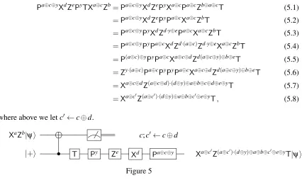
PZ=ZP,PX=XZP,TZ=ZT,TX=XZPT,P2=ZandPa⊕b=Za·bPa+b(fora,b∈ {0,1}). 1. We start with the “X-teleportation” of [47], which is easy to verify (Figure 4).
|ψi c
|+i • Xc|ψi
Figure 4: Circuit identity: “X-teleportation.”
2. Then we substitute the inputXaZb|
ψifor the top wire. We add the gate sequenceT,Py,Ze,Xd,
Pa⊕c⊕yto the output (Figure 5). ByFigure 4, the outcome is given byPa⊕c⊕yXdZePyTXa⊕cZb|ψi.
Pa⊕c⊕yXdZePyTXa⊕cZb=Pa⊕c⊕yXdZePyXa⊕cPa⊕cZb⊕a⊕cT (5.1) =Pa⊕c⊕yXdZePyPa⊕cXa⊕cZbT (5.2) =Pa⊕c⊕yPyXdZd·y⊕ePa⊕cXa⊕cZbT (5.3) =Pa⊕c⊕yPyPa⊕cXdZd·(a⊕c)Zd·y⊕eXa⊕cZbT (5.4) =P(a⊕c)⊕yPyPa⊕cXa⊕c⊕dZd(a⊕c⊕y)⊕b⊕eT (5.5) =Zy·(a⊕c)Pa⊕cPyPyPa⊕cXa⊕c⊕dZd(a⊕c⊕y)⊕b⊕eT (5.6) =Xa⊕c⊕dZ(a⊕c⊕d)·(d⊕y)⊕a⊕b⊕c⊕d⊕e⊕yT (5.7) =Xa⊕c0Z(a⊕c0)·(d⊕y)⊕a⊕b⊕c0⊕e⊕yT, (5.8)
where above we letc0←c⊕d.
XaZb|ψi c;c0←c⊕d
|+i • T Py Ze
Xd Pa⊕c⊕y Xa⊕c0Z(a⊕c0)·(d⊕y)⊕a⊕b⊕c0⊕e⊕yT|
ψi
Figure 5
3. Next, we note that, because diagonal gates commute with control, the circuit of Figure 5 is equivalent to the one inFigure 6.
XaZb|ψi c;c0←c⊕d
ZePyT|+i •
Xd Pa⊕c⊕y Xa⊕c0Z(a⊕c0)·(d⊕y)⊕a⊕b⊕c0⊕e⊕yT|
ψi
Figure 6
4. We note that theXd on the bottom wireaftertheCNOTcan be moved to the bottom wirebefore
theCNOT, as long as we add anXdto the top wire after theCNOT. (Figure 7.)
XaZb|
ψi Xd c;c0←c⊕d
XdZePyT|+i • Pa⊕c⊕y Xa⊕c0Z(a⊕c0)·(d⊕y)⊕a⊕b⊕c0⊕e⊕yT|
ψi
Figure 7
5. Finally, sincec0=c⊕d, yet the measurement resultcundergoes anXd, these two operations cancel out, and we obtain the final circuit as inFigure 8.
We note that a more direct proof of correctness forFigure 8is possible, but that our intermediate
XaZb|ψi c
XdZePyT|+i • Pa⊕c⊕y Xa⊕cZ(a⊕c)·(d⊕y)⊕a⊕b⊕c⊕e⊕yT|
ψi
Figure 8
5.1 Correctness of theT-gate gadget in the test runs
The correctness of theT-gate gadget in theX-test run ofFigure 2is straightforward: theCNOTflips the bit in the top wire if and only ifd=1, while thePxhas no effect on the computational basis states. The correctness ofFigure 3is derived from theX-teleportation ofFigure 4. Since the diagonal gatesZandP
commute with control, they can be seen as acting on the output qubit. Furthermore, usingP2=Zand the fact thatXhas no effect on|+i, we get the final circuit inFigure 3.
6
Completeness
SupposeCis a yes-instance ofQ-CIRCUIT. SupposePfollows the protocol honestly. Then we have the following.
1. In the case of a computation run, the output bit,ccomphas the same distribution as the output bit of
C(|0ni), thusV accepts with probability at least 2/3.
2. In the case of anX-test run and in the case of aZ-test run (by the identities and observations from the previous sections),V accepts with probability 1.
Given that each run happens with probability 1/3, we get thatV accepts with probability at least 2/3+ (1/3)·(2/3) =8/9.
6.1 Auxiliary qubits for theT-gate gadget
In the protocol for theT-gate gadget (Figure 1), we assume the verifier can produce auxiliary qubits of the formXdZePyT|+i. We now show that this is equivalent to requiring the verifier to generate auxiliary qubits of the formZePyT|+i, as claimed inTheorem 3.3. This can be seen by the following equation, which holds up to global phase.
XdZePyT|+i=Ze⊕dPy⊕dT|+i. (6.1) The above can be seen easily since, up to global phase,XT|+i=ZPT|+i, andXP=ZPX. The analysis for the cased=1, follows.
XZePyT|+i=ZeXPyT|+i (6.2)
=ZeZyPyXT|+i (6.3)
=Ze⊕yPyZPT|+i (6.4)
Thus, the verifier chooses a classical x uniformly at random, and if x=1, the verifier re-labels the auxiliary qubits according toEquation (6.1).
7
Soundness
As discussed inSection 1.3, the main idea to prove soundness is to analyze an entanglement-based version of theInteractive Proof System 1. We present the EPR-based version (Section 7.1), and argue why the completeness and soundness parameters are the same. Then, we analyze a general deviating proverP∗
in the EPR-based version and show how to simplify an attack (Section 7.2). We then analyze the case of a test run (Section 7.4) and of a computation run (Sections 7.5). InSection 7.6, we show how this completes the proof of our main theorem (Theorem 3.3).
An interesting consequence of the analysis in this section is that it implies that, if we are willing to have the prover and the verifier share entanglement, then the protocol reduces to a single round. (However, in this case, the work of the verifier becomes more important; one can wonder if the verifier is still “almost-classical”.) Another interesting observation is that sequential repetition is not required (parallel repetition suffices), due to the fact that the analysis makes use of the Pauli twirl (seeSection 7.2), which would also be applicable to the scenario of parallel repetition.
7.1 EPR-based protocol
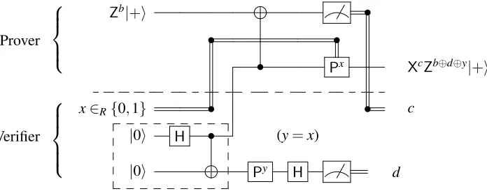
In this version of the quantum-prover interactive proof system (Interactive Proof System 2),allquantum inputs sent by the verifier are half-EPR pairs, andallclassical messages sent by the verifier are random bits. The actions related to choosing between test and computation runs are doneafterthe interaction with the server. For theT-gate, this can be done as shown inFigures 9,10and11.
XaZb|ψi •
Prover • •
• Px Xa0Zb0T|
ψi
x∈R{0,1} • • c
Verifier |0i H • (d∈R{0,1},y=a⊕c⊕x)
|0i T Py⊕d Zd H e
Figure 9: Entanglement-based protocol for aT-gate (computation run). This protocol performs the same computation as the protocol inFigure 1. The output is obtained from the output ofFigure 1
by usingy=a⊕c⊕x. The circuit in the dashed box prepares an EPR-pair. Here, a0=a⊕c and
Xa|0i •
Prover • •
• Px Xd|0i
x∈R{0,1} • • c=a⊕d
Verifier |0i H •
|0i d
Figure 10: Entanglement-based protocol for aT-gate (X-test run). This protocol performs the same computation as the protocol inFigure 2. The circuit in the dashed box prepares an EPR-pair. As in
Figure 2, we include an additionalverificationthatc=a⊕d.
Zb|+i •
Prover • •
• Px XcZb⊕d⊕y|+i
x∈R{0,1} • • c
Verifier |0i H • (y=x)
|0i Py H d
Figure 11: Entanglement-based protocol for aT-gate (Z-test run). This protocol performs the same computation as the protocol inFigure 3. The circuit in the dashed box prepares an EPR-pair.
We therefore defineVEPRas a verifier that delays all choices until after the Prover has returned all
messages (i. e., as the verifier inInteractive Proof System 2). That the soundness parameter is the same
forInteractive Proof Systems 1and2follows from the following series of transformations, each of which
preserves the probability of accept/reject.
1. The quantum communication from the verifier to the prover inInteractive Proof System 1can be generated instead by preparing EPR pairs, sending half and then immediately measuring in the appropriate basis to obtain the required qubit. Call this Interactive Proof System 1.1.
2. Starting from Interactive Proof System 1.1, by a change of variable, we can specify the classical messagexto be random in each of theT-gate gadgets. This determinesy, and the operationPy, that is conditioned ony(for the computation andZ-test run) can be applied immediately before the verifier’s measurement. Call this Interactive Proof System 1.2.
3. In Interactive Proof System 1.2, the prover and verifier operate on different subsystems. Their operations therefore commute and we can specify that the Verifier delays his operations untilafter
Since each transformation above preserves the soundness, and since the completeness parameter is unchanged, from now on, we can focus on establishing the soundness parameter forInteractive Proof
System 2.
7.2 Simplifying a general attack
In this section, we derive a simplified expression for a general deviating prover for our Interactive Proof System. We show that without loss of generality, we can rewrite the actions of any deviating prover as the honest prover’s actions, followed by an arbitrary cheating map. But first, as a technicality, we consider Interactive Proof System 3, which is closely related toInteractive Proof System 2, but where the prover is unitary and show (Lemma 7.2) that a bound on the soundness of Interactive Proof System 3 implies a bound on the soundness ofInteractive Proof System 2.
Definition 7.1. We defineInteractive Proof System 3asInteractive Proof System 2, but with aunitary
prover. To be more precise, the prover (say, Pq) in Interactive Proof System 3 performs the same operations as the prover inInteractive Proof System 2, but does not perform any measurements: instead,
Pqsends qubits to the verifier, sayVEPRq , who immediately measures them in place of the prover, and then continues according to theInteractive Proof System 2.
Lemma 7.2. Interactive Proof Systems 2 and 3 have the same completeness, and furthermore, an upper bound on the soundness parameter for Interactive Proof System 3 is an upper bound on the soundness parameter for Interactive Proof System 2.
Proof. It follows immediately by definition that Interactive Proof Systems 2 and 3 have the same completeness parameter. For soundness, suppose that in Interactive Proof System 3, the probability that
VEPRq accepts while interacting withany Pq∗is at mosts. Suppose for a contradiction that there is aP∗for
Interactive Proof System 2, such thatVEPRaccepts with p>s.
Using polynomial overhead, we obtainP]meas∗ fromP∗via purification (all actions ofP]meas∗ are unitary, except a one-qubit register is measured each time the protocol requires a classical message to be sent to the verifier). The probabilitypof acceptance is unchanged.
Furthermore, starting with P∗, we define fP∗ as a prover for Interactive Proof System 3, which
behaves likeP]meas∗ , but instead of measuring messages to be sent to the verifier, it sends qubits, which are immediately measured byVEPRq , as per Interactive Proof System 3. The probabilitypthat the verifier in Interactive Proof System 3 accepts, when interacting withfP∗is the same as the probability that the
verifier inInteractive Proof System 2accepts, when interacting withP∗. This contradicts p>s, and proves the claim.
Next, we show that, in Interactive Proof System 3, without loss of generality, we can assume that the prover’s actions are the honest unitary ones, followed by a general attack. In order to see this, for a
t-round protocol (involvingtrounds of classical interaction), define a cheating prover’s actions at roundi
Interactive Proof System 2 Verifiable quantum computation with trusted auxiliary states- EPR version LetCbe given as ann-qubit quantum circuit in the universal set of gatesX,Z,CNOT,H,T.
1. The verifier prepares|Φ+i⊗nand sends half of each pair to the prover. These registers are identified with theinputregisters.
2. For each auxiliary qubit required in theH- andT-gate gadgets, the verifier prepares|Φ+iand sends half of each pair to the prover.
3. The prover executes the gate gadgets. The verifier records the classical communication and responds with random classical bits (when required).
4. The prover returns a single bit of output,cto the verifier.
5. The verifier randomly chooses to execute one of the following three runs (but does not inform the prover of this choice).
A. Computation Run
A.1. Measure the remaining input register halves in the computational basis. Take the initial
X-encryption key to be the measurement outcomes (set theZ-key to 0).
A.2. For each gateGinC: perform the key updates for theX,Z,CNOTandHgates. For the
Tgadget, taking into account the classical messages received and sent inStep 3, perform the measurement and key update rules for theT-gadget (Figure 9).
A.3. V decrypts the output bitc; let the result be ccomp. V accepts ifccomp=0; otherwise
reject.
B. X-test Run
B.1. Measure the remaining input register halves in the computational basis. Take the initial
X-encryption key to be the measurement outcomes (set theZ-key to 0).
B.2. For each gateGinC: perform the key updates for theX,Z,CNOTandHgates. For the
Tgadget, taking into account the classical messages received and sent inStep 3, perform the measurement, key update rules and tests for theT-gadget (Figure 10).
B.3. V decrypts the output bitc; let the result beccomp.V accepts ifccomp=0andif no errors
were detected inStep B.2; otherwise reject.
C. Z-test Run
C.1. Measure the remaining input register halves in the Hadamard basis. Take the initial
Z-encryption key to be the measurement outcomes (set theX-key to 0).
C.2. For each gateGinC: perform the key updates for theX,Z,CNOTandHgates. For the
Tgadget, taking into account the classical messages received and sent inStep 3, perform the measurement, key update rules and tests for theT-gadget (Figure 11)
Thus the actions of a general proverP∗are given as the follows.
ΦtHt. . .Φ1H1Φ0H0. (7.1)
SinceH0, . . . ,Ht are unitary, we can rewriteEquation (7.1).
ΦtHt. . .Φ3H3Φ2H2Φ1H1Φ0H0=ΦtHt. . .Φ3H3Φ2H2(Φ1H1Φ0H1∗)H1H0 (7.2)
=ΦtHt. . .Φ3H3(Φ2H2Φ1H1Φ0H1∗H2∗)H2H1H0 (7.3)
=ΦtHt. . .(Φ3H3Φ2H2Φ1H1Φ0H1∗H2∗H3∗)H3H2H1H0 (7.4)
= (ΦtHt. . .Φ3H3Φ2H2Φ1H1Φ0H1∗H2∗H3∗. . .H
∗
t)Ht. . .H3H2H1H0.
(7.5)
Thus, by denoting a general attack by
Φ=ΦtHt. . .Φ3H3Φ2H2Φ1H1Φ0H1∗H2∗H3∗. . .Ht∗, (7.6)
and the map corresponding to the honest prover asH=Ht. . .H3H2H1H0, we get that without loss of
generality, we can assume that the prover’s actions are the honest ones, followed by a general attack:
ΦH. (7.7)
Taking {Ek} to be Kraus terms associated withΦ, and supposing a total ofmqubit registers are involved, we get that the system after interaction withP∗, where the initial state is
Φ+
Φ+
⊗m
= 1 2m
2m−1
∑
i,j=0|iiihj j| (7.8)
(here, we include the classical random bits, as they are uniformly random and therefore we can repre-sent them as maximally entangled states), and where the verifier has not yet performed the gates and measurements, can be described as
1 2m
∑
k
∑
i,j(I⊗EkH)|iiihj j|(I⊗H∗Ek∗). (7.9)
For a fixedk, we writeEkandEk∗in the Pauli basis:
Ek=
∑
Qαk,QQ and Ek∗=
∑
Q0
αk∗,Q0Q0. (7.10)
(To simplify notation, we assume throughout thatQ,Q0 ranges overPm.) By the completeness relation, we have:
∑
k∑
Q|αk,Q|2=1. (7.11)
When it is clear from context, we drop the “k” subscript, thus denoting
Ek=
∑
QαQQ and Ek∗=
∑
Q0
αQ∗0Q0. (7.12)
In the following sections, we analyze the probability of acceptance, as a function of the type of run and of the prover’s attack. ByLemma 7.2, a bound on the acceptance probability gives a bound on the acceptance probability inInteractive Proof System 2(which is a bound on the acceptance probability of
7.3 Conventions and definitions
In addition to the convention of representing an attack as inEquation (7.9), in the followingSections 7.4–
7.5, we use the following conventions.
1. The circuitCthat we consider is already “compiled” in terms of theHgates as inSection 4.4(the identityH=HPHPHPHis already applied).
2. The number ofT-gate gadgets ist(each such gadget uses two auxiliary qubits—one representing an auxiliary quantum bit, and one representing a classical bitx), and the number of qubits in the computation isn. Thus we havem=2t+n.
3. In theT-gate gadget, the auxiliary wire is swapped with the measured wire immediately before the measurement. This way, we may picture that only auxiliary qubits are measured as part of the computation, and that the data registers for the input represent the computation wires throughout. 4. Given the system as inEquation (7.9), we suppose that the firstT-gate gadget uses the first EPR pair as auxiliary quantum bit, and the second EPR pair as a qubit representing the classical bit (and so on for the followingT-gadgets). The lastnEPR pairs are the data qubits, and we suppose that at the end of the protocol, the last data qubit is the one that is measured, representing the output. 5. Normalization constants are omitted when they are clear from context.
Finally, we definebenignandnon-benignPauli attacks, based on their effect on the protocol. As we will see, benign attacks have no effect on the acceptance probability (because all qubits are either traced-out or measured in the computational basis). However, non-benign attacks may influence the acceptance probability.
Definition 7.3. For a fixed PauliP∈Pm, we call itbenign ifP∈Bt,n, whereBt,n is the set of Paulis acting onm=2t+nqubits, such that themeasuredqubits in the protocol are acted on only by a gate in {I,Z}. Using the above conventions, this means thatBt,n={{{I,Z} ⊗P}⊗t⊗Pn−1⊗ {I,Z}}. A PauliP
is callednon-benignif at least onemeasuredqubit in the protocol is acted on only by a gate in{X,Y}. In analogy to the set of benign Paulis, we denote the set of non-benign Paulis acting onm=2t+nqubits asB0t,n.
7.4 In the case of a test run
Based on the preliminaries ofSection 7.2andSection 7.3, we now bound the probability of acceptance of the test runs, by describing the effect of the attack on the entire system, and considering which attacks are detected by the test runs (essentially, we show inLemma 7.4that all non-benign Pauli attacks are detected by one of the test runs).
Lemma 7.4. Consider the Interactive Proof System 2 for a circuit C on n qubits and with t T-gate gadgets, with attack {Ek} (with each Ek=∑Qαk,QQ), and suppose a test run is applied. Let Bt0,nbe the
set of non-benign attacks. Then with the following probability, the verifier rejects
1 2
∑
k Q∑
∈B0t,n
|αk,Q|2. (7.13)
the auxiliary qubitiis an encrypted version of|0i(hi=0) or|+i(hi=1). We note that, by the properties of the protocol,hi=0 in anX-test run if and only ifhi=1 in aZ-test run.
In the case of anX-test, the system that we obtain after the verifier has performed measurements that prepare the encrypted auxiliary qubits and the computation wire is
∑
d1...dt∈{0,1} x1...xt∈{0,1}
Ph1·x1Hh1Xd1|0ih0|Xd1Hh1P∗h1·x1⊗Xx1|0ih0|Xx1
⊗ · · ·
⊗Pht·xtHhtXdt|0ih0|XdtHhtP∗ht·xt⊗Xxt|0ih0|Xxt⊗
∑
a1...an∈{0,1}Xa1|0ih0|Xa1⊗ · · · ⊗Xan|0ih0|Xan
⊗ |d1. . .dt,x1. . .xt,a1. . .anihd1. . .dt,x1. . .xt,a1. . .an|. (7.14)
Note that we have appended a 2t+nqubit register, which is held by the verifier and that contains a classical basis state representing the key.
In the case of aZ-test, the system that we start with is
∑
d1...dt∈{0,1} x1...xt∈{0,1}
Ph1·x1Hh1Xd1|0ih0|Xd1Hh1P∗h1·x1⊗Xx1|0ih0|Xx1
⊗ · · ·
⊗Pht·xtHhtXdt|0ih0|XdtHhtP∗ht·xt⊗Xxt|0ih0|Xxt
⊗
∑
b1...bn∈{0,1}Zb1|+ih+|Zb1⊗ · · · ⊗Zbn|+ih+|Zbn
⊗ |d1. . .dt,x1. . .xt,b1. . .bnihd1. . .dt,x1. . .xt,b1. . .bn|. (7.15)
We claim that, replacing thePandP∗gates with the identity inEquation (7.14)andEquation (7.15), we obtain expressions for the system for each test run, respectively, at theendof the application of the honest unitary. This essentially follows by construction; for completeness we review the case of each gate gadget below.
CNOT-gate. As discussed inSection 4.2, in both theX-test andZ-test, aCNOTgate, when applied
to the computation registers (the lastnregisters), will have no effect (up to a relabelling of the Paulis, as computed by the key update). Thus a simple change of variable reverts the system to an expression identical to its prior state.
H-gate. As given inSection 4.4, the application of theHgate to the computation registers will, up to a
T-gate as part of anX-test. Suppose aT-gate is applied in theX-test run, on qubit j, using an auxiliary qubiti(i=1. . .t). Suppose furthermore that qubit jhas undergone anevennumber ofHgates, so that
hi=0, and the system that the prover acts upon for theT-gate gadget, together with the relevant key register is
∑
di,xi,aj∈{0,1}Xdi|0ih0|Xdi⊗Xxi|0ih0|Xxi⊗Xaj|0ih0| jX
aj⊗
di,xi,aj
di,xi,aj
. (7.16)
Applying thePx andCNOTas in the honest computation has very little effect on the system; it only causes a key update:
∑
di,xi,aj∈{0,1}Xdi|0ih0|Xdi⊗Xxi|0ih0|Xxi⊗Xaj⊕di|0ih0| jX
aj⊕di⊗
di,xi,aj⊕di
di,xi,aj⊕di
. (7.17)
As per our convention, we swap the first and last registers, so that the data wire remains in its position:
∑
di,xi,aj∈{0,1}Xaj⊕di|0ih0|Xaj⊕di⊗Xxi|0ih0|Xxi⊗Xdi|0ih0| jX
di⊗
aj⊕di,xi,di
aj⊕di,xi,di
. (7.18)
Next, a change of variable shows that the expression is unchanged:
∑
di,xi,aj∈{0,1}Xdi|0ih0|Xdi⊗Xxi|0ih0|Xxi⊗Xaj|0ih0| jX
aj⊗
di,xi,aj
di,xi,aj
. (7.19)
T-gate as part of aZ-test. Suppose aT-gate is applied in theZtest run, on qubit j, using an auxiliary
qubiti(i=1. . .t). Suppose furthermore that qubit jhas undergone anevennumber ofHgates, so that
hi=1, and the system that the prover acts upon for theT-gate gadget, together with the relevant key register is
∑
di,xi,bj∈{0,1}PxiZdi|+ih+|ZdiP∗xi⊗Xxi|0ih0|Xxi⊗Zbj|+ih+| jZ
bj⊗
di,xi,bj
di,xi,bj
. (7.20)
Applying thePxandCNOTas in the honest computation changes the system by canceling out thePx i and causing a key update:
∑
di,xi,bj∈{0,1}Zbj⊕di⊕xi|+ih+|Zbj⊕di⊕xi⊗Xxi|0ih0|Xxi⊗Zbj|+ih+| jZ
bj
⊗
bj⊕di⊕xi,xi,bj
bj⊕di⊕xi,xi,bj
. (7.21)
As per our convention, we swap the first and last registers, so that the data wire remains in the last position:
∑
di,xi,bj∈{0,1}Zbj|+ih+|Zbj⊗Xxi|0ih0|Xxi⊗Zbj⊕di⊕xi|+ih+| jZ
bj⊕di⊕xi
⊗bj,xi,bj⊕di⊕xi
bj,xi,bj⊕di⊕xi
. (7.22)
Next, a change of variable shows that the expression is unchanged, except that thePandP∗gates are removed:
∑
di,xi,bj∈{0,1}Zdi|+ih+|Zdi⊗Xxi|0ih0|Xxi⊗Zbj|+ih+| jZ
bj⊗
di,xi,bj
di,xi,bj
Final expression before an attack. In the case that anoddnumber ofHgates have been applied to a data wire, the protocol specifies that we should temporarily swap the roles of theX-test andZ-test runs for theT-gates that immediately follow. In this case, the data qubits and computation will be exactly those considered in the two cases above, but with the roles of theX-test andZ-test exchanged; the same analysis thus applies. For both theX-test andZ-test, we iteratively apply the various cases above (depending on the circuit). Since it is the case that all computation wires eventually have anevennumber ofH-gates applied, we can write down an expression for the outcome for theX-test run:
∑
d1...dt∈{0,1} x1...xt∈{0,1}
Hh1Xd1|0ih0|Xd1Hh1⊗Xx1|0ih0|Xx1
⊗ · · ·
⊗HhtXdt|0ih0|XdtHht⊗Xxt|0ih0|Xxt
⊗
∑
a1...an∈{0,1}Xa1|0ih0|Xa1⊗ · · · ⊗Xan|0ih0|Xan
⊗ |d1. . .dt,x1. . .xt,a1. . .anihd1. . .dt,x1. . .xt,a1. . .an|. (7.24)
In the case of aZ-test, an expression for the outcome is
∑
d1...dt∈{0,1} x1...xt∈{0,1}
Hh1Xd1|0ih0|Xd1Hh1⊗Xx1|0ih0|Xx1
⊗ · · ·
⊗HhtXdt|0ih0|XdtHht⊗Xxt|0ih0|Xxt
⊗
∑
b1...bn∈{0,1}Zb1|+ih+|Zb1⊗ · · · ⊗Zbn|+ih+|Zbn
⊗ |d1. . .dt,x1. . .xt,b1. . .bnihd1. . .dt,x1. . .xt,b1. . .bn|. (7.25)
Applying the attack, decryption and measurement. Next, we apply the attack for a fixedk, as given by
Ek=
∑
QαQQ and Ek∗=
∑
Q0
αQ∗0Q0, (7.26)
followed by the verifier’s decryption, trace and measurement. For the registers that are traced out, we assume that they are decrypted and measured. Furthermore, since they are traced out, we can assume that the quantum auxiliary registers withhi=1 are measured in the diagonal basis. We let
Q=P1⊗Q1⊗P2⊗Q2⊗ · · · ⊗Pt⊗Qt⊗R1⊗ · · · ⊗Rn, (7.27) withPi,Qi,Rj∈P1(i=1. . .t,j=1. . .n) and similarly, let
Q0=P01⊗Q01⊗P
0
2⊗Q02⊗ · · · ⊗P
0
t⊗Q0t⊗R
0
1. . .R0n, (7.28)
For theX-test run, conditioned on outcomesi`(whereh`=0), andk1, . . . ,knthe system becomes
∑
(h`=1∧
i`∈{0,1}),
jm∈{0,1}
∑
Q,Q0αQαQ∗0
∑
d1...dt∈{0,1} x1...xt∈{0,1}
hi1|Xd1Hh1P1Hh1Xd1|0ih0|Xd1Hh1P01Hh1Xd1|i1i ⊗ hj1|Xx1Q1Xx1|0ih0|Xx1Q01Xx1|j1i
⊗ · · · ⊗
hit|XdtHhtPtHhtXdt|0ih0|XdtHhtP0tHhtXdt|iti ⊗ hjt|XxtQtXxt|0ih0|XxtQ0tX xt|j
ti
⊗
∑
a1...an∈{0,1}hk1|Xa1R1Xa1|0ih0|Xa1R01Xa1|k1i ⊗ · · · ⊗ hkn|XanRnXan|0ih0|XanR0nX an|k
ni. (7.29)
Applying the classical Pauli twirl (Lemmas 2.2and2.3), we obtain that the cross terms of the attack vanish, leaving as expression
∑
(h`=1∧
i`∈{0,1}),
jm∈{0,1}
∑
Q
|αQ|2
hi1|Hh1P1Hh1|0ih0|Hh1P1Hh1|i1i ⊗ hj1|Q1|0ih0|Q1|j1i
⊗ · · ·
⊗hit|HhtPtHht|0ih0|XdtHhtPtHht|iti ⊗ hjt|Qt|0ih0|Qt|jti
⊗
hk1|R1|0ih0|R1|k1i ⊗ · · · ⊗ hkn|Rn|0ih0|Rn|kni. (7.30)
Recall that in anX-test run, the verifier rejects if a measurement result on an auxiliary qubit with
hi=0 decrypts to the value 1, or if the output decrypts to the value 1. Thus, applying the above to all terms in{Ek}, we get that the probability that the verifier rejects is given by
∑
k∑
Q∈B1|αk,Q|2, (7.31)
whereB1is the set of 2t+n-qubit Paulis withPi∈ {X,Y}(i=1. . .t)wheneverhi=0, or withRn∈ {X,Y}. A similar calculation shows that for theZ-test run, conditioned on outcomesi`(whereh`=1), and k1, . . . ,knthe system becomes
∑
(h`=0∧
i`∈{0,1}),
jm∈{0,1}
∑
Q
|αQ|2
hi1|Hh1P1Hh1|0ih0|Hh1P1Hh1|i1i ⊗ hj1|Q1|0ih0|Q1|j1i
⊗ · · ·
⊗hit|HhtPtHht|0ih0|XdtHhtPtHht|iti ⊗ hjt|Qt|0ih0|Qt|jti
⊗
hk1|R1|+ih+|R1|k1i ⊗ · · · ⊗ hkn|Rn|+ih+|Rn|kni. (7.32)
Recall that in aZ-test run, the verifier rejects if a measurement result on an auxiliary qubit withhi=0 decrypts to the value 1. Thus, applying the above to all terms in{Ek}, we get that the probability that the verifier rejects is given by
∑
k∑
Q∈B2whereB2is the set of 2t+n-qubit Paulis withPi∈ {X,Y}(i=1. . .t)wheneverhi=0.
Since each test is executed with probability 1/2, and sincehi=0 in theX-test run if and only ifhi=1 in theZ-test run, we obtain that the probability that the verifier rejects is
1 2
∑
k Q∑
∈B0t,n
|αk,Q|2. (7.34)
7.5 In the case of a computation run
Again using the preliminaries ofSection 7.2andSection 7.3, we now analyze soundness in the case of a computation run. First, we determine the effect of a bit flip on the measured qubit in theT-gate gadget
(Section 7.5.1), then we do an analysis for the case that the computation run consists in a singleT-gate
gadget (Section 7.5.2). This is extended to full generality inSection 7.5.3, where we give a lower bound (as a function of the attack and of the underlying computation) on the probability that the verifier rejects in a computation run (seeLemma 7.8).
7.5.1 Effect of a bit flip on a measured qubit
InLemma 7.5, we establish the effect of a bit flip on the measured qubit in theT-gate gadget.
Lemma 7.5. The error induced by anX-gate on the measured qubit in theT-gate gadget inFigure 9is to introduce an extraXZPon the output.
Proof. AnX-gate on the measured qubit inFigure 1will cause the bottom wire to receive the correction
Pa⊕c⊕y⊕1(instead ofPa⊕c⊕y). SincePa⊕c⊕y⊕1=PZa⊕c⊕yPa⊕c⊕y, the following shows how we can use we use and revise the calculation fromEquation (5.1)–Equation (5.8).
Pa⊕c⊕y⊕1XdZePyTXa⊕cZb=PZa⊕c⊕yPa⊕c⊕yXdZePyTXa⊕cZb (7.35) =PZa⊕c⊕yXa⊕c⊕dZ(a⊕c⊕d)·(d⊕y)⊕a⊕b⊕c⊕d⊕e⊕yT (7.36) =Xa⊕c⊕dZ(a⊕c⊕d)·(d⊕y)⊕a⊕b⊕c⊕d⊕e⊕yZa⊕c⊕yZa⊕c⊕dPT (7.37) =Xa⊕c⊕dZ(a⊕c⊕d)·(d⊕y)⊕a⊕b⊕c⊕ePT. (7.38) We note furthermore that theX-gate on the measured qubit causes the Pauli key to be updated asc←c⊕1. Starting with the right-hand side ofEquation (7.38), we thus obtain
Xa⊕c⊕d⊕1Z(a⊕c⊕d⊕1)·(d⊕y)⊕a⊕b⊕c⊕e⊕1PT=Xa⊕c⊕dZ(a⊕c⊕d)·(d⊕y)⊕a⊕b⊕c⊕d⊕e⊕y(XZP)T. (7.39) Comparing withEquation (5.8), we thus see that the effect is to applyXZP.
7.5.2 TheT-gate protocol under attack
Lemma 7.5) will be applied to the computation wire. The Pauli twirl plays again an important part in simplifying a general attack to a convex combination of Pauli attacks. This analysis (Lemma 7.6) is used as the inductive step in the proof of the general case as analysed inSection 7.5.3(seeLemma 7.7).
Lemma 7.6. InInteractive Proof System 2, consider a circuit consisting in a singleT-gate, applied to a data wire which is initially an encryption ofρ. Consider a term in the attack {Ek}, given by Q=P1⊗Q1,
Q0=P01⊗Q01, acting on the auxiliary qubits (P1,Q1,P01,Q01∈P1). Then in the case P1⊗Q16=P10⊗Q01,
this term simplifies to0, whereas otherwise the effect is to apply EδP1Ton the data, while maintaining a
uniform encryption, with the key held by the verifier. (Here, Q∈P1, andδQ=0if Q∈ {I,Z}andδQ=1
otherwise.)
Proof. Suppose the honest circuit of the prover is applied, followed by an attack and the coherent correction of the verifier, which is then followed by a measurement of auxiliary qubits. We consider the effect of a Pauli attackQ=P1⊗Q1,Q0=P01⊗Q01, acting on the auxiliary qubits (P1,Q1,P01,Q01∈P1).
(Strictly speaking this is not a full attack, but instead, ignoring the coefficient, it corresponds to one term in the expansion of the full attack as given by{Ek}.) When a bit flip occurs on the top wire (i. e., when
P1∈ {X,Y}) inFigure 9, then the outcome undergoes an errorE=XZPas given byLemma 7.5. The
above is summarized inFigure 12.
XaZb|ψi P1 •
Prover • Q1 •
• Px Xa0Zb0EδP1T|ψi
x∈R{0,1} • • c
Verifier |0i H • (d∈R{0,1},y=a⊕c⊕x)
|0i T Py⊕d Zd H e
Figure 12: An attack P1⊗Q1 on a single T-gate gadget (computation run). Here, a0 =a⊕c and
b0= (a⊕c)·(d⊕y)⊕a⊕b⊕c⊕e⊕y.
In order to give a mathematical expression forFigure 12, we use the circuit identity inFigure 7
(according to which the measurement outcomecundergoes an encryption and decryption withd). First we consider the caseδP1 =δP10. Applyingy=a⊕c⊕x, and considering the trace of the auxiliary qubits, we get the following expression
∑
i,j∈{0,1}a,b,c,d,
∑
e,x∈{0,1}hi|XdP1Xd|cihc|XdP01Xd|ii ⊗ hj|XxQ1Xx|0ih0|XxQ01X
x|
ji⊗
Xa⊕cZ(a⊕c)·(d⊕x)⊕a⊕b⊕c⊕e⊕xEδP1T
ρT∗E∗δP1Z(a⊕c)·(d⊕x)⊕a⊕b⊕c⊕e⊕xXa⊕c