www.theoryofcomputing.org
Locally Checkable Proofs
in Distributed Computing
Mika Göös
Jukka Suomela
Received August 20, 2012; Revised November 3, 2016; Published November 29, 2016
Abstract: We studydecision problemsrelated tograph propertiesfrom the perspective of
nondeterministic distributed algorithms. For ayes-instance there must exist aproof that can be verified with a distributed algorithm: all nodes must accept a valid proof, and at least one node must reject an invalid proof. We focus onlocally checkable proofsthat can be verified with a constant-time distributed algorithm. For example, it is easy to prove that a graph is bipartite: the locally checkable proof gives a 2-coloring of the graph, which only takes 1 bit per node. However, it is more difficult to prove that a graph isnotbipartite—it turns out that any locally checkable proof requiresΩ(logn)bits per node.
In this paper we classify graph properties according to their local proof complexity, i. e., how many bits per node are needed in a locally checkable proof. We establish tight or near-tight results for classical graph properties such as the chromatic number. We show that the local proof complexities form a natural hierarchy of complexity classes: for many classical graph properties, the local proof complexity is either 0,Θ(1),Θ(logn), or poly(n)bits per node. Among the most difficult graph properties are proving that a graph is symmetric (has a non-trivial automorphism), which requiresΩ(n2)bits per node, and proving that a graph
isnot3-colorable, which requiresΩ(n2/logn)bits per node. Any property of connected graphs admits a trivial proof withO(n2)bits per node.
ACM Classification:C.2.4, F.1.3
AMS Classification:68M14, 68Q15, 68Q25, 68Q85, 03F20
Key words and phrases:nondeterminism, distributed computing, locality, graphs
1
Introduction
This paper studiesdecision problemsrelated tograph propertiesfrom the perspective of distributed graph algorithms. In distributed graph algorithms, the nodes of an unknown communication network (modeled as a graph) work together in order to solve graph problems related to the structure of the communication graph itself. As argued by Fraigniaud in his PODC 2010 keynote talk [10], the appropriate model for distributedyes–noverification is the following:
• For ayes-instance, all nodes must output 1. • For ano-instance, at least one node must output 0.
Intuitively, if we have an acceptable input, all nodes will be happy, and if we have an invalid input, at least one node has to raise the alarm.
Our focus is on distributed verification that is madelocally, by using aconstant-timedistributed algorithm [21,29]. Throughout this paper, we follow the convention that the running time of a distributed algorithm equals the number of synchronous communication rounds. In particular, in a local algorithm all nodes stop afterO(1)communication rounds and announce their outputs. Equivalently, each node makes itsyes–nodecision based on its constant-radius neighborhood in the communication graph.
Recall that agraph propertyis a family of graphs that is closed under isomorphism. We say that a graph propertyPislocally checkableif it can be checked by a local algorithm. That is, there exists a local algorithm, calledverifier, that accepts allyes-instancesG∈Pand rejects allno-instancesG∈/P.
Examples. An easy example of a locally checkable property is determining if a given connected graph is Eulerian: it is sufficient that each node outputs 1 if its degree is even, and 0 otherwise.
Another example is checking if a given graph is a line graph. If the nodes have unique identifiers, a constant-time verifier can check that the graph does not contain any of the nine forbidden subgraphs in Beineke’s [5] characterization of line graphs.
However, local checkability as such does not seem to lead to an interesting complexity theory—for many well-studied graph properties, it is often easy to show that they arenotlocally checkable. The key insight of Korman et al. [15,16,18,19] is to study locally checkableproofs.
1.1 Locally checkable proofs
To illustrate the idea of locally checkable proofs, we start with a canonical example. Consider the problem of checking if a given graph is bipartite. This is not a locally checkable property—indeed, if we consider odd vs. even cycles, we can see that any verifier that solves the problem must have the running timeΩ(n).
The concept of locally checkable proofs is related to locally checkable properties as the familiar complexity classNPis related to the classP. If a problem is inNP, thenyes-instances have a concise proof that can be verified inP. Similarly, if the problem is inLCP(f), thenyes-instances have a concise proof with at mostf(n)bits per node and the proof itself is checkable with a local algorithm. Equivalently, we can interpret locally checkable proofs asnondeterministiclocal algorithms: in the algorithm, each node can nondeterministically guess f(n)bits.
1.2 Contributions
The main contributions of this paper are the following:
1. We define the classLCP(f)that consists of graph properties that admit locally checkable proofs of size f(n)bits per node. This model is related to those studied by Korman et al. [15,16,18,19] and Fraigniaud et al. [11], but strictly stronger than both; seeSection 3.
2. We catalog graph properties according to their local proof complexities, and we show that the LCP(f)classes form a natural hierarchy of decision problems. In particular, there are natural graph properties that separate the following levels of the hierarchy: LCP(0),LCP(O(1)),LCP(O(logn)), andLCP(poly(n)).
We refer toTables 1and2for a summary. Table 1catalogs the complexity of verifyinggraph properties(given a graphG, prove thatG∈P), whileTable 2catalogs the complexity of verifying
solutions to graph problems(given a graphGand a solutionX to graph problemP, prove that the solution is correct).
3. We argue thatLogLCP=LCP(O(logn))is a particularly good candidate for a complexity class of independent interest. The class is robust to variations in the exact definition of theLCPhierarchy. Many graph properties are contained inLogLCPand not contained inLCP(o(logn)).
4. We present proof techniques that can be used to derive tight and near-tight lower bounds for the local proof complexity. We show how to apply tools from other fields of computer science and mathematics: results in extremal graph theory, fooling set arguments from the field of communica-tion complexity, and gadgets that are typical inNP-hardness proofs. Here we mention, in particular, our tight proof-size lower bound ofΩ(logn)for non-bipartiteness and related graph properties, and a near-tight lower bound ofΩ(n2/logn)for non-3-colorability.
2
Definitions and examples
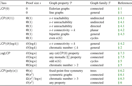
Class Proof sizes Graph propertyP Graph familyF References
LCP(0) 0 Eulerian graphs connected § 1
0 line graphs general § 1
LCP(O(1)) Θ(1) s–treachability undirected § 4.1
Θ(1) s–tunreachability undirected § 4.1
Θ(1) s–tunreachability directed § 4.1
Θ(1) s–tconnectivity=k planar § 4.2
Θ(1) bipartite graphs general § 4.3
Θ(1) evenn(G) cycles
LCP(O(logk)) O(logk) s–tconnectivity=k general § 4.2
O(logk) chromatic number≤k general § 2
LogLCP O(logn) anycoLCP(0)property connected § 7.3
O(logn) any monadicΣ11property connected § 7.5
Θ(logn) oddn(G) cycles § 5
Θ(logn) chromatic number>2 connected § 5
LCP(poly(n)) Θ(n) fixed-point-free symmetry trees § 6.2
Θ(n2) symmetric graphs connected § 6.1
Ω(n2/logn) chromatic number>3 connected § 6.3
O(n2) any property connected § 6
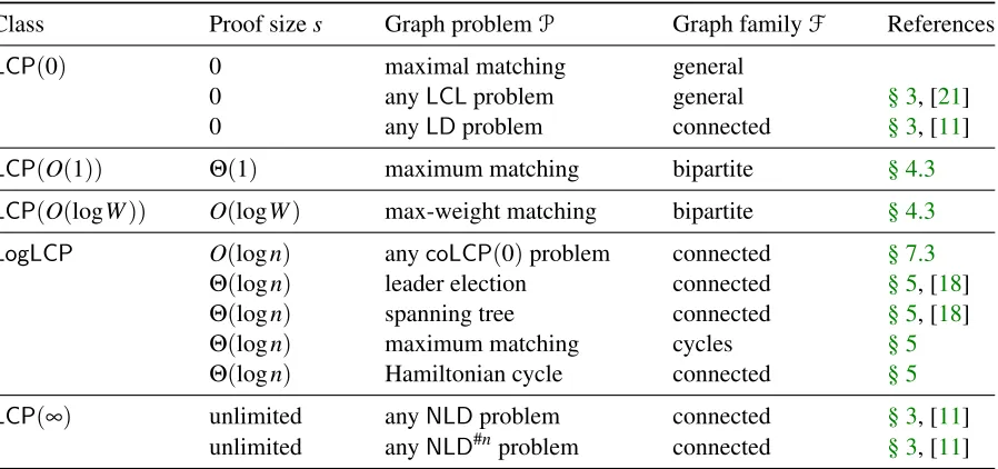
Class Proof sizes Graph problemP Graph familyF References
LCP(0) 0 maximal matching general
0 anyLCLproblem general § 3, [21]
0 anyLDproblem connected § 3, [11]
LCP(O(1)) Θ(1) maximum matching bipartite § 4.3
LCP(O(logW)) O(logW) max-weight matching bipartite § 4.3
LogLCP O(logn) anycoLCP(0)problem connected § 7.3
Θ(logn) leader election connected § 5, [18]
Θ(logn) spanning tree connected § 5, [18]
Θ(logn) maximum matching cycles § 5
Θ(logn) Hamiltonian cycle connected § 5
LCP(∞) unlimited anyNLDproblem connected § 3, [11]
unlimited anyNLD#nproblem connected § 3, [11]
Table 2: The local proof complexity of verifying a solution to graph problemP, when we are promised that the input graph is in graph familyF. HereW is the maximum weight of an edge.
an exception, we studyanonymousmodels without unique identifiers inSections 7.1–7.2.) Depending on the problem that we study, nodes and edges may also be associated with weights, colors, labels, etc.; if this is the case, we say that the graph islabeled, and otherwise it isunlabeled.
2.1 Proofs, verifiers and locality
Proofs. Aproof PforGis a functionP:V(G)→ {0,1}?that associates a binary string with each node ofG. Thesize|P|of a proofPis themaximumnumber of bits in any stringP(v), over allv∈V(G). We writeεfor an empty proof of size 0.
Verifiers. AverifierAis a function that maps each triple(G,P,v)to a binary output 0 or 1. HereG∈F is a graph,P:V(G)→ {0,1}?is a proof, andv∈V(G)is a node ofG. Intuitively,A(G,P,v)is theoutput of nodevif we run the distributed algorithmAin graphGand each nodeu∈V(G)is provided with
input P(u).
Remark 2.1. The issue of whether or not Ais computable (or polynomial-time bounded) is usually immaterial to our considerations. For simplicity, we do not impose any such resource constraints onA; our focus will be on studying the limitations of verifiers arising fromlocality—as defined next.
Local verifiers. For a natural numberr∈Nand a nodev∈V(G), letV[v,r]⊆V(G)be the ball of radius
A verifierAis alocal verifierif there exists a constantr∈Nsuch that A(G,P,v) =A(G[v,r],P[v,r],v)for allG,P,v.
That is, the output of a nodevonly depends on the input in its radius-rneighborhood. Constantris the
local horizonofA. (Alternatively, if we consider Peleg’s [25]LOCALmodel, a local verifier can be defined as a constant-time distributed algorithm: a local verifier with horizonrcan be implemented as a distributed message-passing algorithm that completes inrsynchronous communication rounds.)
2.2 Locally checkable proofs
Agraph propertyP⊆Fis a subset of graphs that is closed under isomorphism. Examples of graph properties include Hamiltonian graphs, Eulerian graphs, bipartite graphs, connected graphs, line graphs, trees, and cycles.
Definition 2.2. A graph propertyP⊆Fadmitslocally checkable proofsof sizes:N→Non familyFif
there is a local verifierAthat satisfies the following properties.
(i) Completeness: IfG∈Pthen there exists a proofP:V(G)→ {0,1}?with|P| ≤s(n(G))such that A(G,P,v) =1 for each nodev∈V(G).
(ii) Soundness:IfG∈F\Pthen for every proofP:V(G)→ {0,1}?there is at least one nodev∈V(G) withA(G,P,v) =0.
That is,yes-instances have a valid proof that is accepted by all nodes, whileno-instances are always rejected by at least one node. If f is a function that associates a valid proofP= f(G)with eachG∈P, we say that the pair(f,A)is aproof labeling scheme.
If a propertyPadmits locally checkable proofs of sizes, we writeP∈LCP(s). We usecoLCP(s)to denote the class of graph properties whose complement is inLCP(s); that is, ifF\P∈LCP(s), we write P∈coLCP(s). The classLogLCPconsists of properties that are inLCP(s)fors=O(logn); we will see inSection 5thatLogLCPadmits many alternative characterizations, which makes it a particularly robust class.
Examples. As we observed inSection 1, Eulerian graphs and line graphs can be verified without a proof, and hence they are inLCP(0). As further observed inSection 1.1, bipartite graphs are not inLCP(0)but they are contained inLCP(1), as they can be verified with one bit of input per node. More generally, if a graph has chromatic number at mostk, we can prove it withdlogkebits per node: simply give a proper
k-coloring as the proof.
2.3 Extension: solutions to graph problems
Formally, agraph problemPassociates any graphG∈Fwith a setP(G)ofsolutions; each solution is a labeled version of graphG. Contrary to the setting of graph properties, there are two natural variants to verifying solutions of graph problemP:
• Strongproof labeling scheme(f,A): for any graphG∈F, for any solutionX∈P(G), there is a locally checkable proof f(X)that is accepted byA, and any incorrect labelingX∈/P(G)is rejected byA.
• Weakproof labeling scheme(f,A): for any graphG∈F, there is at least one solutionX∈P(G) such that there is a locally checkable proof f(X)that is accepted byA, and any incorrect labeling
X ∈/P(G)is rejected byA.
Put differently, in a strong proof labeling scheme, an adversary can choose both the input and the solution, and we must come up with a locally checkable proof. However, in a weak proof labeling scheme, an adversary chooses the input but we can choose a solution. These two notions are different even for natural verification tasks.
Example 2.3(Separating Strong from Weak). Consider the task of verifying whether a set of vertices
C⊆V(G)is a 2-approximation of a minimum vertex cover. It is straightforward to prove that without proof bits, nostrongproof labeling scheme exists for this task, i. e., the approximation ratio achieved by an arbitraryCcannot be determined locally. On the other hand, on bounded-degree graphs there is a constant-time local algorithm [4] that always outputs a setC∗⊆V(G)that is a 2-approximation of the minimum vertex cover—it is thisC=C∗that we can verify without proof bits in theweaksense.
In contrast to the above example, for the remaining problems studied in this paper, the local proof complexities of strong and weak proof labeling schemes are within a constant factor of each other. All proof labeling schemes that we will exhibit are of the strong variety whereas our lower-bound results preclude not only the existence of strong proof labeling schemes for various problems, but also the existence of weak proof labeling schemes.
3
Comparison with other models
Determinism. Our definition of theLCPhierarchy is an extension oflocally checkable labelings(LCL) introduced by Naor and Stockmeyer [21] in their seminal work. Naor and Stockmeyer focus on bounded-degree graphs and constant-size labels, but if we generalize the classLCLin a straightforward manner, we arrive at the classLCP(0).
Our classesLCP(f) with f >0 thus extend the classicalLCLconcept by providing f(n) bits of additional information per node. We have chosen the terminology “LCP” to emphasize this connection, admitting that it is a departure from some of the other terminology available in the literature, as outlined next.
• proof labeling schemesof Korman et al. [15,16,18,19], and • nondeterministic local decisionof Fraigniaud et al. [11].
OurLCPmodel is the strongest among the trio: positive results in the other models imply positive results in our model; this makes our lower-bound results widely applicable. In short, while anLCPverifier algorithm is limitedonly by locality, the verifiers in the other two models have additional restrictions.
3.1 Proof labeling schemes
Theproof labeling schememodel of Korman et al. [15,16,18,19] is inspired by the classical notion of
labeling schemes(see Gavoille and Peleg [12] for a survey). In this model,
(i) the verifier has run-time of 1 communication round, and
(ii) a node cannot see the identifiers nor the input labels of its neighboring nodes.
That is, the output of a single node must be determined on the basis of its own identifier, own input label, own proof label and the proof labels of the neighboring nodes. Thus, an upper bound on the local proof complexity in this model provides an extremely efficient local checking procedure.
Because of these restrictions, verifiers in the proof labeling scheme model are sometimes rather weak. For example, there are simpleLCLproblems that cannot be solved without proof labels in this model: one example is theagreement problemof checking whether all nodes in a connected graph are assigned the same input label [18, Lemma 2.3]; another example is checking whether the input graph is triangle-free. Hence the notion of proof labeling schemes is not a straightforward generalization of the LCLmodel—something ourLCPmodel strives to be.
However, we note that in some cases the gap between the models can be bridged at the cost of an additive proof-size overhead ofΘ(logn)—or however many bits of local data (node identifiers, input labels) are hidden by the restrictions(i)–(ii). This means, for instance, that the two models admit roughly the same analysis at theLCP(poly(n))level (Section 6).
In comparison with prior work related to proof labeling schemes, the main challenges of the present paper can be summarized as follows:
1. Logarithmic lower bounds from prior work do not apply directly. It is harder to fool an LCP verifier that sees all the information available in its constant-radius neighborhood (in particular,
O(logn)-bit identifiers). Therefore we need stronger techniques to proveΩ(logn)proof-size lower
bounds inSection 5.
2. Superlogarithmic lower bounds would apply, but few such bounds are known for graph properties. It seems that the main focus in the prior work has been on problems related to labeled graphs. We can reuse ideas from prior work inSections 6.1–6.2in the context of symmetric graphs, but we are not aware of any prior work related to non-3-colorability that we could apply inSection 6.3.
For logarithmic lower bounds, our novel idea is to invoke an extremal result of Bondy and Simonovits [6] in the context of a “gluing” argument. For superlogarithmic lower bounds, the novel idea is to apply the
3.2 Nondeterministic local decision
Independently of our work, Fraigniaud et al. [11] have also studied nondeterminism (along with random-ness) in the context of distributed decision problems. Here, the major difference to our model is that the local proofsP:V(G)→ {0,1}?are not allowed to depend on the identifier assignment onG. This implies, for example, that many leader election problems are not solvable at all in their model, no matter how largePis (cf.Section 7.1).
To connect the results of Fraigniaud et al. to our work, let us defineLCP0(f)similarly toLCP(f)but restricted to computable properties of connected graphs. With this notation, the classLDof local decision problems defined by Fraigniaud et al. is equal toLCP0(0). The nondeterministic variants ofLDare called NLDandNLD#n; in the latter class each node knows the total number of nodes in the graph. It turns out that our classLCP0(∞)is equal toNLD#n: both classes contain all computable properties of connected
graphs. Hence using the separation results of Fraigniaud et al. we have
LCP0(0) =LD(NLD(NLD#n=LCP0(∞).
While Fraigniaud et al. place one class between the extreme ends ofLCP0(0)andLCP0(∞), our work
introduces an entire hierarchy ofLCP(f)classes.
4
Problems in
LCP
(O(
1
))
As a warm-up, this section gives examples of graph properties and graph problems that admit locally checkable proofs of sizeO(1)but for which there is no locally checkable proof of size 0. We will see that many fundamental problems related to graph connectivity are in this class.
4.1 Reachability
To ask meaningful questions about connectivity in theLCPmodel, we require that two nodessandtare always distinguished in the input graphG; that is, we have the promise that there is exactly one node with labelsand exactly one node with labelt. It is easy to see that inLCP(0)we cannot check whether there is a path fromstotinG. However, many questions related to reachability and connectivity are in LCP(O(1)).
Let us first consider thes–t reachabilityproblem in an undirected graphG, i. e., proving that there is a path fromstot. This problem admits a locally checkable proof of size 1: we find a shortest path fromsto
tinG, define thatU⊆V consists of all nodes on the shortest path, and setP(v) =1 iffv∈U. A verifier can locally check that: (i)s,t∈U; (ii)sandthave unique neighbors inU; and (iii) everyu∈U\ {s,t} has exactly two neighbors inU[14, p. 130].
Interestingly, the above method breaks down in directed graphs because of back-edges. In graphs of maximum degree∆, one can still give an easy upper bound ofO(log∆)by using edge pointers in the proof labeling to describe a path fromstot, but it is an open problem whether directeds–treachability is inLCP(O(1))for general graphs (see also Ajtai and Fagin [1]).
and there is no (directed) edge fromStoT. Such a partition can be encoded with 1 bit per node, and it can be verified locally.
4.2 Connectivity
As a natural generalization of reachability, we can study the s–t connectivity of undirected graphs; throughout this text, we focus on thevertex connectivity. By extending the techniques of Korman et al. [18] we can show that graphs withs–tconnectivity equal tokadmit locally checkable proofs of size
O(logk). Here we assume thatkis given as input to all nodes (or, equivalently, thatkis a global constant). If and only if the vertex connectivity is exactlyk, then by Menger’s theorem [7, p. 62] we can find (i) a partitionS∪C∪T ofV such thats∈S,t∈T, and|C|=k, and (ii)k vertex-disjoint s–t paths
p1,p2, . . . ,pk such that|C∩pi|=1. Without loss of generality, we can assume that each pi is locally minimal in the sense that it cannot be made shorter without colliding with the other pathspj, j6=i.
The proof labelP(v)encodes whetherv∈S,v∈C, orv∈T. Moreover, in the proof labelP(v)of a vertexv∈pi\ {s,t}, we include the path indexi(in binary) and also the distance ofvfromsmodulo 3: this allows us to store the orientation on the pathpi. The local verifier can verify that:
1. Nodessandthave exactlykneighbors labeled with path indices 1,2, . . . ,k. 2. Eachv∈pi\ {s,t}has exactly one predecessor and one successor alongpi. 3. We haves∈S,t∈T, and there is no edge betweenSandT.
4. Eachv∈Cis on a path pi, its predecessor along piis inSand its successor is inT.
If the above checks go through, the structure encoded by the proofPcontains exactlykdisjoints–tpaths. It may contain some oriented cycles insideSor insideT as well, but this is sufficient to convince the verifier that the connectivity ofsandtis at leastk. Moreover, if a path crossesC, its color changes from
StoT; its color cannot change back toS, and it cannot disappear without reachingt. Hence the above checks are also sufficient to convince the verifier that the size of thes–t separatorCis at mostk. In summary,s–t-connectivity has to be equal tok.
Finally, we note that the sole source for theO(logk)label size was the need to store the path indices. However, on planar graphs, only 3 path indices suffice to tell adjacent paths from one another; an adaptation of the above method gives a constant size proof in the case of planar graphs.
4.3 Bipartite matching
Whilemaximalmatchings can be verified without any proofs, verifyingmaximum-cardinalitymatchings requires some auxiliary information. In this section we studybipartitegraphs; later inSection 5.4we will show that the methods below break down onnon-bipartitegraphs.
Maximum matching. To construct a constant-size proof Pfor maximum matchings on a bipartite graphGwe can use König’s theorem [7, p. 35], which states that, on bipartite graphs, the maximum size of a matching equals the minimum size of a vertex cover. Indeed, take any minimum vertex cover
exactly one endpoint inC. This proves that maximum matchings in bipartite graphs are inLCP(1), as the size ofPis 1.
Maximum-weight matching. Generalizing the above example, we can use linear programming duality to prove that in an edge-weighted bipartite graphG, a subset of edgesM⊆E(G)is a maximum-weight matching. Associate a variablexe≥0 with each edgee∈E, and a dual variableyv≥0 with each node
v∈V. Letwe∈Nbe the weight of edgee, and letAbe the vertex-edge incidence matrix of graphG.
Recall (e. g., [24, §13.2]) that matrixAand its transposeA> are totally unimodular, and hence there are integral vectorsxandythat maximize∑ewexesubject toAx≤1 (primal LP) and minimize∑vyv subject toA>y≥w(dual LP). Each maximum-weight matchingMcorresponds to an optimal integral solutionx
of the primal LP, and we can use an optimal dual solutionyas a proof; for each nodev∈V, the proof consists of a binary encoding of the valueyv. To verify the proof, it is sufficient to check thatxandy satisfy the complementary slackness conditions. If the weights are integers from 0,1, . . . ,W, then we can find an optimal dual solution such thatyv∈ {0,1, . . . ,W}for each nodev. Hence the size of the proof is
O(logW)bits.
5
Problems in
LogLCP
In this section we give examples of graph properties and graph problems that admit locally checkable proofs of sizeO(logn)but for which there is no locally checkable proof of sizeo(logn). That is, these problems are inLogLCPbut not in any lower level of theLCPhierarchy. We begin with positive results that directly build on prior work—a key ingredient is the observation that spanning trees in connected graphs are inLogLCP. After that, we give our new lower-bound results.
5.1 Positive results
A spanning tree is not locally checkable, but Korman et al. [18] show that any spanning treeT can be equipped with a proof of sizeO(logn)that, for each vertexv, consists of (i) the identity of a particular vertexa,the root, and (ii) the distance fromvtoainT. Such a proof can be locally verified by checking that the root-distance atais 0, and that for each vertexv(i) all neighbors ofvagree on the identity of the root, and (ii) the root-distance decreases at exactly one neighbor ofvinT and increases at other neighbors.
A spanning tree equipped with a locally checkable proof is a versatile tool. For example, consider theleader electionproblem: there has to be exactly one node that is labeled as the leader. In connected graphs, we can verify any solution to the leader election problem by constructing a spanning tree that is rooted at the leader.
Spanning trees can be also used to prove that the graph is acyclic: we simply show that each component is a tree. Hamiltonian cycles and Hamiltonian paths can be verified by using the same technique: a Hamiltonian path can be interpreted as a spanning tree.
sum of the counter values of its children plus 1. Hence graph properties such as having an odd number of nodes are also inLogLCP.
InLogLCP, we can also show that the chromatic number of a connected graph is larger than 2 (i. e., the graph is not bipartite). To construct a proof, first find an odd cycle in the graph—such a cycle exists if and only if the graph is non-bipartite. Then select one of the nodes of the cycle as the leadera. Construct a spanning tree rooted ata; this way the verifier can check that there exists exactly one leader. Then propagate a node counter along the cycle, starting and ending ata; this way the leader node can be convinced that it is indeed part of an odd cycle.
5.2 Negative results: overview
We will now prove the following theorem.
Theorem 5.1. The following graph properties and graph problems do not admit locally checkable proofs of size o(logn): graphs with odd number of nodes, non-bipartite graphs, spanning trees, and leader election.
Hence these are examples of problems whose containment inLogLCPis tight: their local proof complexity is exactlyΘ(logn).
Proof sketch. The negative results build on the same basic idea. We will consider graph properties on cycles. We will assume that there is a proof labeling scheme(f,A)witho(logn)-bit proofs. We will take severalyes-instances—each of them is a short cycle—and inspect the encoding produced by f. Then we will show that some of theyes-instances are necessarilycompatible with each otherin the following sense: we can take several short cycles andglue them togetherto form a longer cycle; the unique identifiers and the proof labels are inherited from the short cycles, and each node of the long cycle will be locally indistinguishable from a node of a short cycle. Hence the verifier will accept the long cycle, as it has to accept all short cycles.
However, even though the short cycles areyes-instances, the long cycle will be ano-instance. For example, in the case of non-bipartiteness, each short cycle has an odd number of nodes, but the long cycle is composed of an even number of short cycles, and is therefore ano-instance. In the case of leader election, each short cycle has one leader node, while the long cycle will contain multiple leaders, and is therefore an invalid solution. Similar ideas can be applied to many other lower bounds.
5.3 The proof
LetFbe a family of graphs that contains (at least) all cycles. In each graph G∈F, we may have a constant number of bits of auxiliary information per node (colors, labels, etc.). LetP⊆Fbe a graph property. Assume that(f,A)is a proof labeling scheme for propertyPthat useso(logn)-bit proofs. Fix an integer constantk≥2. Letnbe a sufficiently large positive integer. We will assume thatn-cycles (with appropriate auxiliary information) are inP.
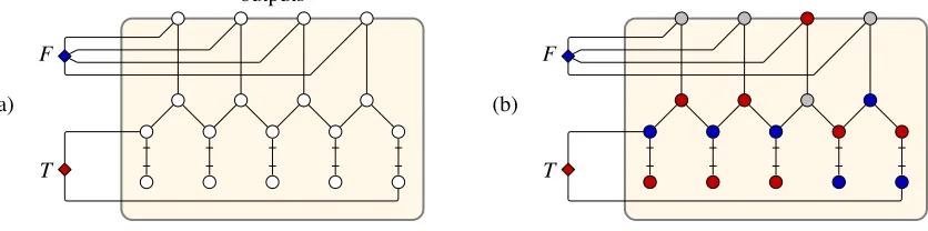
Our plan is to show that we can always findk yes-instances, each of which is ann-cycle, and we can glue them together to form akn-cycle that inherits the proof labels (and auxiliary information, if any) from theyes-instances. VerifierAwill accept eachn-cycle, and therefore it will also accept thekn-cycle. For an example, refer toFigures 1and2.
Partitioning the space of identifiers. First, split n=nA+nB, where nA =bn/2c and nB =dn/2e. Fix any partition of the set of identifiers{1, . . . ,n2}into 2nsubsets a1, . . . ,an,b1, . . . ,bn so that each
a∈A:={a1, . . . ,an}is of sizenA, and eachb∈B:={b1, . . . ,bn}is of sizenB. We denote bya[i](resp.,
b[i]) thei-th identifier ina(resp.,b) in the natural order.
For example, if n=10, we have nA =nB =5. We can choose the partition a1 ={1,2, . . . ,5},
a2={6,7, . . . ,10}, . . . ,b10={96,97, . . . ,100}. In this casea2[1] =6,b10[2] =97, etc.
Family ofyes-instances. Next, we define a family ofyes-instancesC(a,b)indexed by pairs(a,b)∈
A×B. DefineC(a,b)to be then-cycle that contains the nodesain increasing order followed by the nodesbin decreasing order, completing the cycle. That is,a[1]andb[1]are adjacent, as area[nA]and
b[nB]; seeFigure 1a. Note thatV(C(a,b))andV(C(a0,b0))are disjoint ifa=6 a0andb6=b0.
Augment eachC(a,b)with auxiliary information such thatC(a,b)is inP, if necessary; letLab(v)∈ {0,1}?be the bit string associated with nodev∈V(C(a,b)). For example, if we are interested in the leader election problem, label exactly one node in eachC(a,b)as the leader: select a nodeu∈V(C(a,b)) and setLab(u) =1 andLab(v) =0 for allv6=u. We can consider either the best-case or the worst-case choice of the leader, thus covering both weak and strong proof labeling schemes.
Recording proof bits. Now we make use of the assumption that propertyPadmitso(logn)-bit proofs. Apply ftoC(a,b)to construct a locally checkable proofPabof sizeo(logn). For each nodev∈V(C(a,b)), letPab0 (v) = (Lab(v),Pab(v)). Finally, define
c(a,b) = Pab0 (a[2r+1]),Pab0 (a[2r]), . . . ,Pab0 (a[1]),Pab0 (b[1]),Pab0 (b[2]), . . . ,Pab0 (b[2r+1]) .
That is,c(a,b)consists of all auxiliary information and all proof bits that are available within distance 2r+1 from the nodea[1]orb[1]inC(a,b); seeFigure 1a. By assumption, we have o(rlogn)bits of information inc(a,b).
Finding compatible cycles. Now let Kn,n = (A∪B,E) be the complete bipartite graph with E = {{a,b}:a∈A,b∈B}. We define an edge coloring ofKn,nas follows: the color of the edge{a,b} ∈Eis
b[1] b[2] b[3] b[4] b[5] C b’[1] b’[2] b’[3] b’[4] b’[5] a a’ b b’ b[1] b[2] b[3] b[4] b[5] edge colour
c(a, b)
b’[1]
b’[2]
b’[3]
b’[4]
b’[5]
C(a’, b’)
c(a’, b’)
a[1]
a[3]
a[4]
a[5]
a[2]
c(a’, b’)
(c) (a) a[1] a[3] a[4] a[5] a[2] a’[1] a’[3] a’[4] a’[5] a’[2] a’[1] a’[3] a’[4] a’[5] a’[2]
C(a, b)
c(a, b)
(b)
a[1] b[1]
b[2] b[3] b[4] b[5] a[3] a[4] a[5]
C(a, b)
a[2]
c(a, b)
Figure 1: An illustration of the Ω(logn) lower-bound construction; here n=10, r=1, andk =2. (a) Construction of the cycleC(a,b). We consider the leader election problem in this example; hence precisely one node is highlighted to indicate the leader node. (b) A monochromatic 2k-cyclea,b,a0,b0in
and the number of distinct colors inKn,nis therefore smaller than 3 √
n. Hence there is a subset of edges
H⊆E such that|H|>|E|/√3n=n5/3and all edges ofHhave the same color.
Now we can apply the result due to Bondy and Simonovits [6]: for any k≥2 and for a suffi-ciently largen, the subgraph(A∪B,H)necessarily contains a 2k-cycle. Let the nodes of the cycle be
a1,b1,a2,b2, . . . ,ak,bkin this order, such thatai∈Aandbi∈Bfor eachi. As all edges of the cycle have the same color, we have
c(a1,b1) =c(a2,b2) =· · ·=c(ak,bk) =c(a1,bk) =c(a2,b1) =· · ·=c(ak,bk−1).
For convenience, defineb0=bk andak+1=a1.
Gluing. Next, we glue together then-cyclesC(a1,b1),C(a2,b2), . . . ,C(ak,bk)to construct akn-cycle
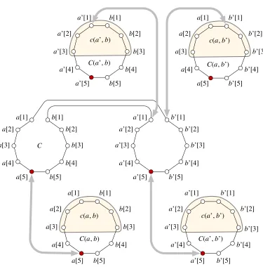
C. That is, we take the node-disjoint graphsC(ai,bi), remove the edges{ai[1],bi[1]}for eachi, and add {bi−1[1],ai[1]}for eachi>1. For each nodev∈V(C), we inherit the auxiliary informationL(v)and the proof bitsP(v)from the cyclesC(ai,bi). The gluing process is illustrated inFigure 1c for the casek=2. We have two compatiblen-cycles,C(a,b)andC(a0,b0), and we connecta[1]tob0[1]anda0[1]tob[1].
Analysis. It remains to argue that the computation ofAonCwith the labelsLand proofPis accepting. To see this, pick a vertexv∈V(C). Then there is anisuch thatv∈V(C(ai,bi)). Ifvis far fromai[1]and
bi[1], then the local neighborhood ofvlooks identical inCandC(ai,bi); asC(ai,bi)is ayes-instance,v accepts the input. Ifvis nearbi[1], then the local neighborhood ofvlooks identical inCandC(ai+1,bi), which is anotheryes-instance. Similarly, ifvis nearai[1], then its local neighborhood looks identical in
CandC(ai,bi−1), which is also ayes-instance (seeFigure 2for an illustration). In all cases,vaccepts the input. Thus thekn-cycleCis accepted by all nodes. IfC∈/P, we have a contradiction, and we can conclude that the graph propertyPdoes not admit locally checkable proofs of sizeo(logn).
5.4 Implications
Now we can give concrete examples of graph properties and graph problemsPfor whichC∈/P, provided that we choose the parameterskandnproperly:
• Non-bipartite graphs: We can select an oddnandk=2.
• Leader election: It is sufficient to choose k=2. Then eachC(a,b) contains exactly one node labeled as a leader andCcontains two nodes.
• Spanning trees: Again, we can choosek=2. The spanning tree in eachC(a,b)contains all edges ofE(C(a,b))except one, i. e., it is a spanning path. The solution encoded inCconsists of two disjoint paths, and is therefore not a spanning tree.
We can also apply the same construction to counting problems: to give a simple example, if we choose an oddnand an evenk, thenn(C(a,b))is odd whilen(C)is even.
b[1] b[2] b[3] b[4] b[5] C b’[1] b’[2] b’[3] b’[4] b’[5] b[1] b[2] b[3] b[4] b[5] b’[1] b’[2] b’[3] b’[4] b’[5]
C(a, b’)
c(a, b’)
b’[1]
b’[2]
b’[3]
b’[4]
b’[5]
C(a’, b’)
c(a’, b’)
a[1] b[1] b[2] b[3] b[4] b[5] a[3] a[4] a[5]
C(a’, b)
a[2]
c(a’, b)
a[1] a[3] a[4] a[5] a[2] a[1] a[3] a[4] a[5] a[2] a’[1] a’[3] a’[4] a’[5] a’[2] a’[1] a’[3] a’[4] a’[5] a’[2] a’[1] a’[3] a’[4] a’[5] a’[2]
C(a, b)
c(a, b)
node. The solution inherited fromC(a,b)toChas thereforekunmatched nodes, and cannot be optimal. Hence all of these problems require proofs of sizeΩ(logn)and the lower bound is tight. This concludes the proof ofTheorem 5.1.
6
Problems in
LCP
(
poly
(n))
In the previous sections, we have seen problems that admit locally checkable proofs of sizeO(log(n)). Now we turn our attention to the problems that require much larger proofs. If the nodes can have arbitrary labels (e. g., weights), it is easy to come up withartificialproblems that require arbitrarily large proofs. However, in this section we will focus on findingnaturalexamples of graph properties that are related to
unlabeledgraphs: we do not have any additional information besides the structure of the graphGand the unique node identifiers.
In connected graphs,anyproperty of unlabeled graphs admits locally checkable proofs of sizeO(n2). We can encode the structure ofGand the unique node identifiers inO(n2)bits; the nodes can verify that their neighbors agree on the structure ofGand that their local neighborhoods match those inG. Finally, the nodes can solve the problem by brute force.
In this section, we will show that there are natural graph properties that requireΩ(n2)-bit proofs. Such problems are the most difficult problems from theLCPperspective—we can only save a constant factor in comparison with the brute-force solution.
6.1 Symmetric graphs
In this section, we fixFto be the family of connected graphs. We say that a graphGissymmetricif it has a non-trivial automorphism, that is, there is an automorphismg:V→V that is not the identity function; otherwise it isasymmetric.
Theorem 6.1. Symmetricity of connected graphs requires locally checkable proofs of sizeΩ(n2).
Proof. To reach a contradiction, assume that there exists a proof labeling scheme(f,A)witho(n2)-bit proofs. To facilitate the proof, we will usecanonical formsof graphs. We associate a canonical formC(G) with any graphG. GraphsGandC(G)are isomorphic; moreover, wheneverGandHare isomorphic, their canonical formsC(G)andC(H)are equal. We assume that the node identifiers of a canonical form areV(C(G)) ={1,2, . . . ,n(G)}. We also define a graph withshifted identifiersas follows: for an integer
i, graphC(G,i)hasV(C(G,i)) ={i+1,i+2, . . . ,i+n(G)}as the set of node identifiers. Moreover, we assume thatg:v7→i+vis an isomorphism fromC(G)toC(G,i). In particular,C(G,0) =C(G).
Now we are ready to give the lower-bound construction. Given two connected graphsG1andG2 withn(G1) =n(G2) =k, we construct a graphG=G1}G2 withV(G) ={1,2, . . . ,3k}as follows: G consists of a copy ofC(G1,k), a copy ofC(G2,2k), and the path(k+1,1,2, . . . ,k,2k+1). That is,G consists of a path that joins graphs that are isomorphic toG1andG2.
Assume thatG1andG2are asymmetric. IfG1andG2are isomorphic, thenG=G1}G2is symmetric: there is a non-trivial automorphism that maps 17→k andk+17→2k+1 and so on. Conversely, ifG
admits a non-trivial automorphismϕ, then, by the construction ofG, we must have thatϕ swapsG1and
LetFkbe a family containing a representative from each isomorphism class of asymmetric connected graphs withk nodes. For anyG1∈Fk, the local verifierAhas to acceptG1}G1, as it is symmetric. Since almost all graphs are connected [7, Cor. 11.3.3] and asymmetric [8], we have
|Fk|= (1−o(1))2( k
2)/k! and log|Fk|=Θ(k2).
Now assume thatk≥2r+1, whereris the local horizon ofA. Consider the proof labels of the nodes inU={1,2, . . . ,2r+1}. There are onlyo(rn2)proof bits inU. Asr=O(1)andn=3k, we have only
o(k2)proof bits inU; for sufficiently largekthis is less than log|Fk|. Hence we must have two different graphsG1,G2∈Fksuch that the labeling scheme assigns the same proof bits to the nodes 1,2, . . . ,2r+1 in bothG1}G1andG2}G2.
Now we can construct the asymmetric graphG=G1}G2. For the nodesk+1,k+2, . . . ,2k we inherit the proof labels from f(G1}G1), and for the nodes 2r+2,2r+3, . . . ,k,2k+1,2k+2, . . . ,3kwe inherit the proof labels from f(G2}G2). For the nodes 1,2, . . . ,2r+1 we use the common labeling of
f(G1}G1)and f(G2}G2). Now the radius-r neighborhood of any node inGlooks identical to the neighborhood of a node inG1}G1orG2}G2. Hence all nodes will accept the input even thoughGis not symmetric, a contradiction.
Remark 6.2. The basic idea of the above proof is similar to Korman et al. [18, Corollary 2.4]. However, Korman et al.’s construction gives a problem related to graphs that are labeled with unique identifiers; it is not a graph property in the usual sense (closed under re-assigning the identifiers).
6.2 Fixed-point-free symmetry on trees
In this section, we fixFto be the family of connected trees. Here, any graph propertyP⊆Fadmits a locally checkable proof of sizeO(n): for each nodevof the treeG∈P, we encode the structure ofGand an index that identifies which node ofGisv; the structure of a tree can be encoded inΘ(n)bits, and the index requiresΘ(logn)bits.
Now we will show that there are properties of unlabeled trees that requireΘ(n)-bit proofs. We will use the following (artificial) problem as an example. We say that a graphGhas afixed-point-free symmetryif there is an automorphism that fixes no nodes, i. e., there is an automorphismg:V(G)→V(G)such that
g(v)6=vfor allv∈V(G).
Theorem 6.3. Trees with a fixed-point-free symmetry require locally checkable proofs of sizeΘ(n).
The proof is analogous to the case of symmetric graphs. The only difference is that we letFk consist of rooted trees withknodes; ifG1,G2∈Fk andkis even, thenG1}G2has a fixed-point-free symmetry if and only ifG1=G2. We have log|Fk|=Θ(k)[28, Seq. A000081]; hence a proof of sizeo(n)bits leads to a contradiction.
6.3 Non-3-colorability
a graph can be colored with 2 colors aΘ(1)-bit proof is sufficient, but to show that a graph cannot be
colored with 2 colors we needΘ(logn)-bit proofs.
In the case of 3-colorings, the difference between the problem and its complement is even more dramatic. Again, constant-size proofs are enough to show that a graph can be colored with 3 colors, as we can give a 3-coloring as a proof. However, to prove that a graph cannot be colored with 3 colors, we need very large proofs, with polynomially many bits per node.
Theorem 6.4. Non-3-colorability requires locally checkable proofs of sizeΩ(n2/logn).
LetFbe the family of connected graphs, and letP⊆Fconsist of graphs that have chromatic number larger than 3. We will show that propertyPdoes not admit locally checkable proofs of sizeo(n2/logn). Recall that any property of unlabeled graphs admits proofs of sizeO(n2); hence the result is almost tight, and shows that non-3-colorability does not have a proof labeling scheme that is substantially better than the brute-force approach.
Proof overview. The template for our lower-bound proof will be thedisjointness problemin two-party communication complexity: two players, Alice and Bob, are given sets Aand B, respectively, and they need to communicate to find out whetherA∩B=∅. It is well-known that this problem has high
communication complexity even in the nondeterministic setting where the players seek to prove that
A∩B=∅; see Example 1.23 and Lemma 2.4 in Kushilevitz and Nisan [20]. Recall also that proving
A∩B6=∅is easy: simply guess an element inA∩B.
Our lower bound graphG=GA,B will have two subgraphsGA and GB that are owned by Alice and Bob, respectively. These subgraphs are connected by someΘ(logn)wires, that, intuitively, allow
nondeterministic communication between the players (via the proof labels). The subgraphsGAandGB are constructed in such a way that if we are given any partial 3-coloringcofGdefined only on the wires ofG, thenccan be extended to 3-coloring ofGA(resp.,GB) if and only ifcencodes, in a certain way, an element inA(resp.,B). This means thatGA,B will be 3-colorable iffA∩B6=∅—or in other words
GA,Bwill be non-3-colorable iffA∩B=∅. A communication complexity argument then implies that the
wires must carry large proof labels.
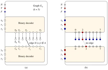
Properties ofGA. Letkbe a positive integer. DefineI={0,1, . . . ,2k−1}. Given a setA⊆I×I, we construct a graphGA, with the following properties:
(i) The total number of nodes inGAisΘ(2k).
(ii) The set of nodesV(GA)contains the following nodes:T,F,N,x0,x1, . . . ,xk−1, andy0,y1, . . . ,yk−1.
Moreover, proper 3-colorings ofGAhave the following properties:
(iii) The nodesT,F, andNhave three different colors. The nodes with the same color asT are said to betrue, those with the same color asFarefalse, and others areneutral.
(v) In any 3-coloring, we must have (x,y)∈A. Conversely, we can find a proper 3-coloring that encodes any(x,y)∈A.
An explicit construction ofGAfollows. In the subsequent analysis the details of the construction are not used outside of the above properties (i)–(v).
Gadgets. We begin with the basic building blocks of GA. In graphGA, nodesT, F, andN form a triangle, ensuring that in any 3-coloring these nodes have different colors.
N T
F
Recall that the nodes with the same color asT are said to betrue, those with the same color asF are
false, and others areneutral. NodesT,F, andNare extensively used in the construction of the following gadgets.
ABoolean gadgethas twoterminals; seeFigure 3. In a proper 3-coloring, exactly one terminal is true and the other terminal is false; conversely, any such assignment is a proper 3-coloring.
Acolor changerhas oneinput nodeand oneoutput node; seeFigure 4. In any proper 3-coloring, a true input implies a true output while a neutral input implies a false output (and a false input is not possible); conversely, any such assignment can be realized as a proper 3-coloring.
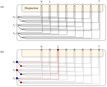
Adisjunction gadgethas a number ofoutput nodes; seeFigure 5. In any proper 3-coloring, at least one output node is true and all other output nodes are neutral; conversely, any such assignment can be realized as a proper 3-coloring. The construction uses Boolean gadgets.
Finally, we construct abinary decoderas illustrated inFigure 6. There arekinput nodes, labeled withx0,x1, . . . ,xk−1, and 2k output nodes, labeled with 0,1, . . . ,2k−1, i. e., with a number inI. In any 3-coloring, each input node is either true or false, while each output node is either true or neutral. The color assignment of the input nodes can be interpreted as a binary encoding of a numberi∈I, and the decoder guarantees that only the output node with labeliis true. Conversely, any such assignment can be realized as a proper 3-coloring. In the construction of the binary decoder, a disjunction gadget ensures that at least one output node is true, while the edges between inputs and outputs ensure that if an output node is true, its index matches the truth assignment of the input nodes. Now we have all basic ingredients for constructing graphGA.
Construction ofGA. The high-level structure of graphGA is shown inFigure 7. There are 2k+3
terminals:T,F,N,x0,x1, . . . ,xk−1, andy0,y1, . . . ,yk−1. There are alsonon-terminalnodesai,bi, andci fori∈I.
The construction contains two binary decoders: one mapping inputsxjto outputsai, and the other mapping inputsyito outputscj. Moreover, there are 2kcolor changers, each of them mapping inputaito outputbi. Finally, we have an edge{bi,cj}if and only if(i,j)∈/A.
= = =
(a) N (b)
Figure 3: (a) Boolean gadget: one terminal is true, one terminal is false. (b) Proper 3-colorings.
= = =
(a) (b)
input
output
N F
Figure 4: (a) Color changer: true7→true but neutral7→false. (b) Proper 3-colorings.
(a)
outputs
T F
(b)
T F
Figure 5: (a) Disjunction gadget with four output nodes. (b) An example of a proper 3-coloring.
(i) aiis true iffi=x; otherwiseaiis neutral, (ii) biis true iffi=x; otherwisebiis false, (iii) ciis true iffi=y; otherwiseciis neutral.
In particular, bothbxandcyare true, and therefore we must have(x,y)∈A. Conversely, for any pair of integers(x,y)∈A, we can construct a proper 3-coloring ofGAsuch the coloring ofxj forms the binary encoding ofxand the coloring ofyjforms the binary encoding ofy.
Construction ofG=GA,B. We have now completed the construction ofGAfor any given setA⊆I×I. In what follows, we denote byG0Aan isomorphic copy ofGA; we use the primed symbolsT0,F0,N0,x0i, andy0ito refer to the terminal nodes ofG0A.
We will need one more gadget: awirethat propagates colors; seeFigure 8. A wirewconsists of 9r
Disjunction (a)
(b)
0 2 7
x0
x1
x2
0 1 7
x0
x1
x2
x0
x1
x2
y0
y1
y2 N T F
Binary decoder Binary decoder
Graph GA (k = 3)
edge if (x,y) ∉A
x0
x1
x2
y0
y1
y2 N T F
0 2 7
0 3 7
no edge
a0 a1 ax a7
c0 c1 cy c7
b0 b1
(a) (b)
Figure 7: (a) The high-level structure of graphGA. (b) An example:(x,y) = (2,3)∈A.
andw(i,j)must have the same color asw(i+1,j).
Given two setsA,B⊆I×I, we construct a graphG=GA,Bthat consists of subgraphsGAandG0Bthat are connected to each other by 2k+1 wires; seeFigure 9. The wires ensure thatGAandG0Bagree on the coloring of the terminals.
In more detail, we label the 2k+1 wires withwT,wx1,wx2, . . . ,wxk, andwy1,wy2, . . . ,wyk. The endpoints of the wires are identified with the nodes of the subgraphsGA andG0Bas follows:
w(1,1) =N and w(3r,1) =N0 for each wirew,
wT(1,2) =T and wT(3r,2) =T0,
wxi(1,2) =xi and wxi(3r,2) =x
0
i for eachi=0,1, . . . ,k−1,
wyi(1,2) =yi and wyi(3r,2) =y
0
i for eachi=0,1, . . . ,k−1.
Analysis. We make the following observations ofG:
(i) The total number of nodes inGisn=Θ(2k).
a’
N’
a N
a’
N’
a N
=
…
a’
N’
a N
…
(a) (b)
a’
N’
a N
=
Figure 8: (a) A wire between terminalsaanda0. (b) An example of a proper 3-coloring.
x’0
x’1
x’2
y’0
y’1
y’2 N’
T’
F’ G’B
x0
x1
x2
y0
y1
y2 N
T
F GA GA,B (k = 3)
wire
(iii) The shortest path from a node ofGA to a node ofG0Bhas length at least 3r−1. In particular, for sufficiently larger, the local neighborhood of any node is a subset ofW∪V(GA)or a subset of
W∪V(G0B).
Moreover, 3-colorings ofGhave the following properties:
(iv) NodesNandN0have the same color, nodesT andT0 have the same color, and nodesF andF0
have the same color. Hence the concepts of true, false, and neutral nodes are well-defined inG.
(v) Nodesxiandx0i have the same color for eachi, and nodesyi andy0i have the same color for each
i. In particular, bothGA andG0Bagree on the encoding of the same pair(x,y), and we must have (x,y)∈A∩B.
It follows thatGA,B has a 3-coloring if and only ifA∩B6=/0. LetA⊆I×Iand let ¯Abe its complement. NowA∩A¯=/0 andG
A,A¯ does not have a 3-coloring; hence it is inP. If we had locally checkable proofs of sizeo(n2/logn), the total number of proof bits inW
would beo(rn2); on the other hand, there areΘ(n2)elements inI×I. Hence for sufficiently largenthere
are two different setsA,B⊆I×Isuch that we have the same proof bits inW for bothGA,A¯ andGB,B¯. Now we are ready to apply a fooling set argument. AsA6=B, we haveA∩B¯6= /0 or ¯A∩B6= /0 (or both). Without loss of generality, assume thatA∩B¯6= /0. HenceGA,B¯ admits a 3-coloring, and it is therefore not inP. But we can construct a proof as follows: the proof bits ofGAare inherited from the proof ofGA,A¯, the proof bits ofGB0¯are inherited from the proof ofGB,B¯, and the proof bits of wires are the same as inGA,A¯ andGB,B¯. Hence each node ofGA,B¯has a local neighborhood that looks identical to a node ofGA,A¯ orGB,B¯. AsGA,A¯ andGB,B¯areyes-instances, all nodes will acceptGA,B¯, a contradiction.
This completes the proof ofTheorem 6.4that non-3-colorability requires proofs of sizeΩ(n2/logn).
For comparison, proofs of sizeO(n2)are trivially sufficient.
7
Structural properties
In the previous sections we have discussedconcrete examplesof graph properties and their local proof complexities. By contrast, the focus of this final section is on the structural propertiesof the LCP hierarchy: We study the sensitivity of ourLCPmodel to the definitional choices made inSection 2. In a similar vein, we will seek alternative characterizations of the classLogLCP. Finally, we give some observations relating ourLCPclasses to other complexity classes.
7.1 Port numbering algorithms
Throughout this paper, we have used the assumption that the local verifier can access the unique identifiers of the nodes (in accordance with Peleg’s [25]LOCALmodel). Furthermore, we have assumed that the proof can depend on the identifier assignment (recall that this convention is not followed by Fraigniaud et al. [11]). In this section we ask what one can locally prove in a setting where node identifiers are not available.
unique identifiers. There is only a port numbering available in the network, i. e., a node of degreed
can refer to its neighbors by integers 1,2, . . . ,d. We refer to Angluin [3] and Suomela [29] for a formal definition of the PN model.
Recall that ifϕ:V(H)→V(G)is acovering map(i. e., an onto graph homomorphism that for each
v∈V(H)maps the neighbors ofvinHbijectively onto the neighbors ofϕ(v)inG), thenHis said to be aliftofG[2,3]. For example, anykn-cycle is a lift of ann-cycle. Furthermore, we say that a property P⊆Fisclosed under liftsifG∈PimpliesH∈Pfor every liftH∈FofG.
A fundamental limitation of a PN algorithmAis that it is fooled by a liftϕ:V(H)→V(G)in the following sense [3,29]: for every local inputP:V(G)→ {0,1}?we have that
A(H,P◦ϕ,v) =A(G,P,ϕ(v)) for allv∈V(H)
for suitable port numberings ofHandG. Thus—regardless of the size ofP—this directly implies that any property that can be locally checked using a PN verifier must be closed under lifts: if each node outputs 1 on(G,P), then each node outputs 1 on(H,P◦ϕ). In fact, the converse holds on connected graphs:
Theorem 7.1. Suppose thatP⊆Fis a property of connected graphs that is closed under lifts. ThenP admits locally checkable proofs of size O(n2)that can be verified using a PN algorithm.
Proof. On input a connected graph H ∈F, the PN verifier for P expects the proof labelP(v) of a nodev∈V(H)to encode a pair(G,ϕ(v)), whereGis a connected graph (without port numbers) having identifiersV(G) ={1, . . . ,n(G)}, andϕ(v)∈V(G)is a distinguished node. Naturally, an honestO(n2)-bit proof will haveP(v) = (H,v)for allv.
We let the PN verifier perform the following checks at a nodev∈V(H). First, we check that all the neighbors ofvhold the same encoding ofGin their proof labels. This ensures that all nodes agree on the encoding ofGsince the input graph is connected. Thenvchecks that degH(v) =degG(ϕ(v))and that
{ϕ(u):uis a neighbor ofvinH}={u:uis a neighbor ofϕ(v)inG}.
These checks guarantee that the mapϕ:V(H)→V(G)is a covering map. Finally, the PN verifier accepts iffG∈P. The soundness of the checking procedure now follows from the assumption thatPis closed under lifts.
7.2 Alternative characterizations ofLogLCP
ALogLCPproof can address individual vertices by theirO(logn)identifiers. Consequently—and in contrast to the discussion above—LogLCPcontains properties that are not closed under lifts (e. g., non-bipartiteness). Next, we show how a little additional input structure can enable a PN verifier to check properties inLogLCP. This shows that the classLogLCPis robust in the sense that we can change our underlying model of distributed computation and yet arrive at exactly the same class of graph properties. We note that the model (3) below is related to the classNLD#nconsidered by Fraigniaud et al. [11].
Theorem 7.2. On connected graphs G, the classLogLCPcoincides with properties that can be locally verified with O(logn)bits in each of the following models:
2. PN with anelected leaderin G.
3. PN with each node being given n(G)as input.
Proof. We show that the above models are equivalent by describing how to pass from one model to another with only an additiveO(logn)overhead in proof size.
(1⇒2 & 3): Using spanning tree methods [18] we already saw inSection 5that (on a connected graph) proving the presence of a unique leader and verifying the number of nodes is inLogLCP.
(2 & 3⇒1): Consider the following attempt at encoding a spanning treeT ofGin the PN model: the
O(logn)proof encodesT together with the root-distances. The problem with this encoding is that since we cannot talk about the identifier of the anonymous root ofT, we cannot verify that such an encoding describes aspanning treerather than a spanning forest. However, we can overcome this tree/forest problem by employing either one of the assumptions (2) or (3): Under (2) we can require that the unique elected leader inGis the root of the spanning tree. Under (3) we can equipT with node counters along the paths towards the root and thus verify that alln(G)nodes are contained in the same tree. Hence, in either of the models (2) or (3) we can build and verify a spanning treeT ofG.
UsingT we can generate unique identifiers for the nodes ofGas follows (cf. ancestor labeling schemes[12]): Do a depth-first traversal onT starting at the root and record in the proof label of a nodev
its discovery timex(v)and finishing timey(v); the identifier of a nodevis then an encoding of the pair (x(v),y(v)). We note that the pairs(x(v),y(v))can be locally checked to be consistent with a depth-first traversal onT—it follows that the node identifiers are globally unique.
Remark 7.3. Fraigniaud et al. [11] describe how arandomizedlocal verifier can check—in a certain probabilistic sense—whether a graph containsat most one leader. This technique provides yet another means to check for the uniqueness of a rooted spanning tree.
7.3 Complementing inLCP(0)
We will now show thatcoLCP(0)⊆LogLCPon connected graphs. The key idea is that we can employ spanning trees to reverse the decision made by anLCP(0)verifier.
LetFbe the family of connected graphs, letP⊆Fbe a graph property inLCP(0), and let ¯P=F\P be the complement ofP. We will show that ¯Padmits a locally checkable proof of sizeO(logn)in graph familyF.
LetAbe a local verifier that checksP; we will useAto design a proof labeling scheme for ¯P. For anyyes-instanceG∈P, we construct a locally checkable proof¯ Pof sizeO(logn)as follows: Select a root nodeawithA(G,ε,a) =0, i. e.,ais a node that rejects the inputG. Then choose an arbitrary spanning treeT rooted ata. LetPconsist of an encoding of(T,a)and a proof of its correctness.
The proof is checked by a local verifier ¯Aas follows. First, ¯Averifies thatT is valid spanning tree rooted ata; in particular, there is a finite path from anyv∈V(G)toa. Second, at the root nodea, verifier
¯
AsimulatesAand checks thatA(G,ε,a) =0.
By construction, a valid proof is accepted by ¯A. Let us now show that we cannot fool ¯A. Consider a
no-instanceG∈/P¯ and any proofP. We have one of the following cases:
2. Pis an encoding of a spanning treeT rooted ata. However,G∈Pand thereforeA(G,ε,a) =1. Hence ¯Aoutputs 0 at the root nodea.
We conclude that for eachG∈P¯ there is a proofPthat is accepted by ¯A, and for eachG∈/P¯ any proofP
is rejected by ¯A. Hence ¯Pis inLogLCP.
7.4 Containment inNPandNP/poly
Comparing classes such asLogLCPandNPis not straightforward. To define theLCPhierarchy, we have used theLOCALmodel, which allows unlimited local computation. Hence if we have unbounded node degrees inG(or unbounded amount of additional information per node in the form of colors or weights), we can easily come up with artificial problems that are inLCP(0)but not inNP.
However, the situation becomes much more interesting if we study bounded-degree graphs; moreover, we will consider properties of unlabeled graphs, i. e., there is no additional information besides the node identifiers and the topology of the graph.
In this restricted case, we can still show that there are problems inLogLCPthat are not contained inNP. Once again, we can resort to spanning tree methods: without loss of generality, we can assume that aLogLCPverifier has access ton=n(G)in any connected graphG. Hence the verifier can solve arbitrarily hard problems concerning the integern, including those that are not inNP(which exist by the hierarchy theorems [23, §7.2]).
However, ifP∈LogLCPis a graph property related to unlabeled bounded-degree graphs, wecan
show thatPis inNP/poly, i. e.,NPwith a polynomial-size non-uniform advice. In a bounded-degree graph, the number of nodes inside the local horizon is bounded by a constant, and hence aLogLCP verifierAuses onlyO(logn)bits of input in total. Thus verifierAcan be encoded as a lookup table of size 2O(logn), which is polynomial inn. We can provide the entire lookup table as the advice stringSto an NP/polymachineM. ThenMmerely guesses theO(nlogn)-bit proofP:V(G)→ {0,1}?, and uses the advice stringSto verify the guess.
7.5 Connections to descriptive complexity
A central result in descriptive complexity theory and one that began the field is Fagin’s [9], [14, Ch. 7] characterization of the classNPas graph properties expressible byexistential second-order formulas
(Σ11)—this is the extension of first-order logic that allows existential quantification over relation symbols
X1,X2, . . .(of any arity). SomeNP-complete graph properties (e. g., 3-colorability) are even expressible bymonadicΣ11 formulas that only quantify over unaryrelation symbols [1,26]. In this section, we
make observations of a connection between theLogLCPclass and the class of graph properties that are expressible by monadicΣ11formulas.
In the study offirst-orderexpressibility, locality is a thematic subject; this is illustrated by Hanf’s theorem and the work of Gaifman [14, Ch. 6]. Building on this work, Schwentick and Barthelmann [27] have shown that on connected graphs, every monadicΣ11formula is equivalent to a formula of the form
ϑ=∃X1∃X2. . .∃Xk∃x∀y:ϕ(X1, . . . ,Xk,x,y),
can be determined whetherGsatisfiesφ(X1,X2, . . . ,Xk,x,y)on the basis of ther-radius neighborhood ofy inG. (More formally, the quantifications inϕ are always of the form∃z:(dist(z,y)≤r∧ψ)or ∀z:(dist(z,y)≤r→ψ), where “dist(z,y)≤r” simply stands for “the distance between zandyis at mostr”.)
Let us consider the familyFof connected graphs. If and only if a graphG∈Fhas propertyϑ, there are unary relationsA1,A2, . . . ,Akand a nodea∈V such thatGsatisfies∀y:ϕ(A1,A2, . . . ,Ak,a,y). For each nodevand each relationAi, encodingAi(v)takes 1 bit. To prove the existence of the nodea, we can use a spanning tree rooted ata; a locally checkable spanning tree requiresO(logn)bits per node (recallSection 5). To check the proof, the verifierAfirst checks the spanning tree, and then evaluates ϕ(A1,A2, . . . ,Ak,a,y)for each nodey. Asϕis local aroundy, the verifierAis a local algorithm. Hence in connected graphs, any monadicΣ11graph propertyPadmits locally checkable proofs of sizeO(logn),
i. e.,P∈LogLCP.
8
Open problems
We conclude by summarizing some open problems raised by our paper. While the local proof complexity as a function of the number of nodesnis now fairly well understood, we left a small gap in the case of non-3-colorability, which is probably a proof artifact.
1. Prove that non-3-colorability is not inLCP(o(n2)).
There are also many open questions related to the local proof complexity as a function of the maximum degree∆:
2. InSection 4.1we saw that directeds–treachability admits locally checkable proofs of sizeO(log∆).
Is there a proof labeling scheme withO(1)-bit proofs?
3. Eulerian tours admit a straightforward proof of sizeO(∆logn), and the lower-bound techniques
ofSection 5imply a lower bound ofΩ(logn). Is there a proof labeling scheme withO(logn)-bit proofs?
If we increase the local horizon of a verifier, can we decrease the proof size? Korman et al. [17] show how this can be done when verifying minimum weight spanning trees. Do such trade-offs exist for all properties inLCP(O(1)), or not:
4. Do we haveLCP(k)(LCP(k+1)for all constantsk∈N?
The analogous question has been answered affirmatively for monadicΣ11expressibility [22].
Perhaps our most nagging question is one that involves another structural property of the class LCP(O(1)). Recall that inSection 7.4it was straightforward to see thatLogLCP*NP. The analogous
question forLCP(O(1))is the following:
It should be noted that in caseFis closed under disjoint unions of graphs, a single componentC⊂Gin a graphG∈Fcan have node identifiers that are not bounded by a polynomial inn(C). In this case, a modification of the Ramsey argument of Naor and Stockmeyer [21, §3] applies to get rid of the identifier dependencies and provesP∈NP.
Acknowledgments
We thank the anonymous reviewers for their helpful comments and suggestions. This work was supported in part by the Academy of Finland, Grants 132380 and 252018, the Finnish Cultural Foundation, and the Research Funds of the University of Helsinki. Most of this work was conducted while the authors were affiliated with the University of Helsinki.
References
[1] MIKLÓSAJTAI ANDRONALDFAGIN: Reachability is harder for directed than for undirected finite graphs. J. Symbolic Logic, 55(1):113–150, 1990. Preliminary version inFOCS’88.JSTOR. 9,28
[2] ALONAMIT, NATHANLINIAL, JI ˇRÍMATOUŠEK,ANDEYALROZENMAN: Random lifts of graphs. InProc. 12th Ann. ACM-SIAM Symp. on Discrete Algorithms (SODA’01), pp. 883–894. ACM Press, 2001. Abstract based on papers inCombinatorica ’02,Combinatorics, Probability and Computing ’06,Random Struct. Algorithms ’02, andCombinatorica ’05. [ACM:365801] 26
[3] DANAANGLUIN: Local and global properties in networks of processors. InProc. 12th STOC, pp. 82–93. ACM Press, 1980. [doi:10.1145/800141.804655] 25,26
[4] MATTI ÅSTRAND AND JUKKA SUOMELA: Fast distributed approximation algorithms for vertex cover and set cover in anonymous networks. In Proc. 22nd Ann. ACM Symp. on Parallelism in Algorithms and Architectures (SPAA’10), pp. 294–302. ACM Press, 2010. [doi:10.1145/1810479.1810533] 7
[5] LOWELLW. BEINEKE: Characterizations of derived graphs. J. Combinatorial Theory, 9(2):129– 135, 1970. [doi:10.1016/S0021-9800(70)80019-9] 2
[6] JOHN A. BONDY ANDMIKLÓSSIMONOVITS: Cycles of even length in graphs.J. Combin. Theory Ser. B, 16(2):97–105, 1974. [doi:10.1016/0095-8956(74)90052-5] 8,12,15
[7] REINHARD DIESTEL: Graph Theory. Springer, Berlin, Germany, 3rd edition, 2005. Official website. 10,18
[8] PAUL ERD ˝OS AND ALFRÉDRÉNYI: Asymmetric graphs. Acta Mathematica Hungarica, 14(3-4):295–315, 1963. [doi:10.1007/BF01895716] 18
[10] PIERRE FRAIGNIAUD: Distributed computational complexities: are you Volvo-addicted or NASCAR-obsessed? In Proc. 29th Ann. ACM Symp. on Principles of Distributed Computing (PODC’10), pp. 171–172. ACM Press, 2010. [doi:10.1145/1835698.1835700] 2
[11] PIERREFRAIGNIAUD, AMOSKORMAN,ANDDAVIDPELEG: Local distributed decision. InProc. 52nd FOCS, pp. 708–717. IEEE Comp. Soc. Press, 2011. To appear in J. ACM. J. ACM version available atauthor’s home page. [doi:10.1109/FOCS.2011.17] 3,5,8,9,25,26,27
[12] CYRILGAVOILLE ANDDAVIDPELEG: Compact and localized distributed data structures. Dis-tributed Computing, 16(2-3):111–120, 2003. [doi:10.1007/s00446-002-0073-5] 8,27
[13] MIKA GÖÖS AND JUKKA SUOMELA: Locally checkable proofs. In Proc. 30th Ann. ACM Symp. on Principles of Distributed Computing (PODC’11), pp. 159–168. ACM Press, 2011. [doi:10.1145/1993806.1993829] 1
[14] NEILIMMERMAN: Descriptive Complexity. Graduate Texts in Computer Science. Springer, Berlin, Germany, 1999.9,28
[15] AMOS KORMAN AND SHAY KUTTEN: On distributed verification. In Proc. 8th Internat. Conf. on Distributed Computing and Networking (ICDN’06), pp. 100–114. Springer, 2006. [doi:10.1007/11947950_12] 2,3,8
[16] AMOSKORMAN ANDSHAYKUTTEN: Distributed verification of minimum spanning trees. Dis-tributed Computing, 20(4):253–266, 2007. Preliminary version inPODC’06. [doi:10.1007/s00446-007-0025-1] 2,3,8
[17] AMOSKORMAN, SHAYKUTTEN,AND TOSHIMITSUMASUZAWA: Fast and compact self stabi-lizing verification, computation, and fault detection of an MST. InProc. 24th Ann. ACM Symp. on Principles of Distributed Computing (PODC’05), pp. 311–320, 2011. To appear in Distributed Computing. [doi:10.1145/1993806.1993866] 29
[18] AMOS KORMAN, SHAY KUTTEN, AND DAVID PELEG: Proof labeling schemes. Distributed Computing, 22(4):215–233, 2010. Preliminary version inPODC’05. [doi:10.1007/s00446-010-0095-3] 2,3,5,8,10,11,12,18,27
[19] AMOSKORMAN, DAVIDPELEG, ANDYOAV RODEH: Constructing labeling schemes through universal matrices. Algorithmica, 57(4):641–652, 2010. Preliminary version in ISAAC’06. [doi:10.1007/s00453-008-9226-7] 2,3,8
[20] EYALKUSHILEVITZ ANDNOAM NISAN:Communication Complexity. Cambridge Univ. Press, Cambridge, UK, 1997. [ACM:264772] 19
[21] MONINAOR ANDLARRYJ. STOCKMEYER: What can be computed locally? SIAM J. Comput., 24(6):1259–1277, 1995. Preliminary version inSTOC’93. [doi:10.1137/S0097539793254571] 2,5,