2249
A Segment Length And Weight Optimized Fuzzy
Time Series For Cloud Load Prediction
Rashmi Singh Lodhi, R. K. Pateriya
Abstract: The ever-growing demand for resources in cloud computing has caused an equal rise in the power consumption of the cloud-based systems. This could be minimized by managing the active resources in a cloud system according to the load pattern. To manage these resources efficiently and effectively, accurate prediction of resource demands is necessary. Because a prior knowledge of load demands may greatly help in deciding that whether a particular resource will be needed in near future or not, and accordingly the operational state (active, sleep, shutdown, and terminated) of resources can be managed. To achieve this, in this paper a fuzzy time series and particle swarm optimization (PSO) based cloud load forecasting method is proposed. The PSO is used here for the optimization of intervals in fuzzy time series. We evaluated the performance of the proposed method with the Google Cluster Dataset. The method also tested for the different forecast intervals and the results show that the proposed technique outperforms previous methods with a considerable margin.
Index Terms: Minimum 7 keywords are mandatory, Keywords should closely reflect the topic and should optimally characterize the paper. Use about four key words or phrases in alphabetical order, separated by commas.
————————————————————
1
INTRODUCTION
Cloudcomputing systems are increasingly being used by industry, government, and academia, due to their ability to provide efficient, versatile, and scalable computational power [1]. Cloud computing platforms offer a wide range of advantages for application deployment, especially the ability to provide pay-per-use pricing schemes for a vast number of resources [2]. Cloud computing uses virtualization technologies to provide infrastructure, application and cloud management facilities [3]. The virtualization platform manages virtual machines (VMs) which runs software or services within a cloud environment. VMs are the virtual instance of a computer system running over a layer abstracted from the actual hardware and generated by logically allocating and organizing the physical resources [3]. The cloud service provider guarantees a minimum level of service quality (QoS), also referred to as the Service Level objective (SLO) [4], [5]. However under complex load conditions, maintaining the SLO is a difficult task [6]. Considering the competitive market conditions it is required to keep the operational cost as low as possible. One of the major contributor in cloud operational cost is electrical power. This is because, (1) improper assignment of workloads over VMs which causes larger task completion time and hence higher energy consumption, (2) keeping the VMs in active state to improve response time and task execution time for upcoming tasks, without even knowing the possibility of upcoming tasks, which causes the power consumption even when VMs are idle. These idle computing resources with their energy consumption adds nineteen billion dollars surplus financial burden [7]. The electrical power requirement of a cloud system can be minimized by proactive control of VMs configuration and state based on current and future workload requirements. In this paper, an optimized interval fuzzy time series based approach is presented to forecast the cloud load. The rest of the paper is structured as follows. Section II gives a brief review of the literature. Section III provides a fuzzy time series and PSO overview.
Section IV describes the architecture of the proposed system. Section V presents the simulation results with detailed analysis. Finally, in section VI conclusion and the possibilities of future work are discussed.
2
LITERATURE
REVIEW
Several techniques have been proposed for cloud data center load prediction. A combine approach using wavelet and support vector machine (SVM) named as WSVM is presented in [9]. The WSVM algorithm exploits the wavelet transform in detecting the frequency related characteristics of workload, and non-linear regression capability of SVM. The algorithm is further extended in [10], using specialized wavelet basis function and weighting the training samples non-uniformly. Furthermore, the tuning of SVM is performed using PSO algorithm. Another combine approach using Evolutionary Algorithm (EA), Kalman Filter and Adaptive Neuro-Fuzzy Inference System (ANFIS) is presented in [11]. A statistical method based approach based on autoregressive integrated moving average (ARIMA) using R (R-Programming Language) forecast package for workload forecasting is presented in [12]. A number of method for time series prediction method such as Autoregressive (AR), Moving Average (MA), Simple Exponential Smoothing, Double Exponential Smoothing, ETS (error, trend, seasonal), Automated ARIMA, and Neural network auto-regression are presented in [13]. The simulation results presented by them shows that the neural network and double exponential methods provide more accurate results compare to other methods. An Artificial Neural Network (ANN) and Self-Adaptive Differential Evolution (SaDE) based approach is presented in [14], where the SaDE is used to train the ANN. An ensemble approach using Fuzzy Neural Network based on Subtractive-Fuzzy Clustering (A combine subtractive clustering with fuzzy c-means) is presented in [15]. In this algorithm the Subtractive-Fuzzy Clustering is used for the estimation of fuzzy rules and other configuration parameters. A pattern fusion model for multi-step-ahead CPU load prediction is presented in [16], in this model firstly the distance of past and present data sequences are calculated using Euclidean and fluctuation pattern distance and then a weighted method along with machine learning algorithm is used to combine these distances and form a predictor. A recurrent neural __________________________________
• Rashmi Singh Lodhi,PhD Scholar, Computer Science and Engineering, Maulana Azad National Institute of Technology (MANIT), Bhopal, India. E-mail: [email protected] • Co-Author name is currently pursuing masters degree
network (RNN) based short term workload forecasting model for is presented in [17], and validated against the regression model, which shows that the recurrent neural network has much better short term forecasting capability. Another recurrent neural network based on long short-term memory (LSTM) architecture is presented in [18]. In this proposal a direct training of recurrent neural network for sequence labelling using new architecture for output layer is also presented. The LSTMtsw an extension to LSTM is which used prediction error moderation to minimize the forecasting error is presented in [19]. In this method the prediction is controlled through the comparison of difference between predicted outputs with actual outputs, so when difference grows beyond a threshold the prediction is stopped until it falls back within acceptable range. To overcome the RNN prediction limitations in [20] an L-PAW algorithm based on deep learning is presented. The comparison of L-PAW with RNN on the real cloud load data trace obtained from Google and Alibaba shows, that L-PAW improves the performance for the long term predictions.
3 FUZZY
TIME
SERIES
Work on time series has made significant progress in coping with accurate prediction for most of the cases. However, in many practical cases the time series sequences seems to involve more noise. In such conditions the traditional time series forecasting fails significantly to achieve desired accuracy. In such cases the fuzzy logic system provides a considerable advantage due to its nature of simultaneously relating the multiple sets via provided conditions. The fuzzy time series concept was firstly introduced by Song et al [21]. Below are the related Fuzzy time series definitions. Before going further we must know the definition of fuzzy series as provided in [21].
3.1 Definition 1
Let a universe of disclosure 𝑌(𝑡)(𝑡 = ⋯ ,0,1,2, … ), be a subset of real numbers ℝ, on which the fuzzy sets 𝑓(𝑡)(𝑖 = 1,2,3 … ) lies, then the 𝐹(𝑡) which, represents the collection of 𝑓(𝑡) will be called a fuzzy time series in the universe of 𝑌(𝑡).
3.2 Definition 2
Assume that only 𝐹(𝑡 − 1) causes the𝐹(𝑡), then this will we denoted as 𝐹(𝑡 − 1) → 𝐹(𝑡), and 𝐹(𝑡) can be defined by a first order model 𝐹(𝑡) = 𝐹(𝑡 − 1) ⊛ 𝑅(𝑡, 𝑡 − 1), where ⊛ is Max-Min operator, and 𝑅(𝑡, 𝑡 − 1) represents the fuzzy relationship between 𝐹(𝑡 − 1) and 𝐹(𝑡).
3.3 Definition 3
The fuzzy time series 𝐹(𝑡) will be called a time invariant only if 𝑅(𝑡, 𝑡 − 1) = 𝑅(𝑡 − 1, 𝑡 − 2), 𝑓𝑜𝑟 ∀ 𝑡, where 𝑅(𝑡, 𝑡 − 1), is a first order model; else it will be called a time variant fuzzy time series.
3.4 Definition 4
The fuzzy logical relationship (FLR) at current state is denoted as 𝐴 → 𝐴, where 𝐴 = 𝐿𝐻𝑆 and 𝐴 = 𝑅𝐻𝑆 corresponds to 𝐹(𝑡 − 1) and 𝐹(𝑡) respectively.
3.5 Fuzzy Time Series Forecasting Model
One of the most common conventional fuzzy time series forecasting model is presented by Chen et al [22] is described
here to explain the working of fuzzy time series. The model requires following steps:
Step 1: At first the universe of discourse is estimated for example, let we have a time series given by 𝑆 = *𝑠 , 𝑠 , … , 𝑠 +, where 𝑀 be the number of samples in the series. Then the universe of disclosure can be estimated as:
𝑈 = *𝑆 , 𝑆 +, #(1)
Where𝑆 and𝑆 are the minimum (min (𝑆)) and maximum (max (𝑆)) values in the series 𝑆.
Step 2: Now the 𝑈 is divided into the equal length of segments. If the segment length is denoted by 𝑙 , then 𝑈 can be divided into 𝑁 segments such as 𝑢, 𝑢 , … 𝑢 , where 𝑁 is calculated as:
𝑁 =𝑆 − 𝑆 𝑙 , #(2)
Using 𝑙 the starting and ending interval of 𝑖 segment can be given as:
𝑢 = ,𝑆 + (𝑖 − 1) × 𝑙, 𝑆 + 𝑖 × 𝑙 -#(3)
Step 3: To each segment 𝑢 , 𝑢 , … 𝑢 assign respective fuzzy linguistic variable𝐴 , 𝐴 , … , 𝐴 .
Step 4: Convert the series 𝑆 into fuzzy series by replacing the each element of 𝑆 through corresponding linguistic variable. Here the corresponding fuzzy variable 𝐴 for an 𝑠 ∈ 𝑆 must satisfy:
𝑆 + (𝑗 − 1) × 𝑙 < 𝑠 ≤ 𝑆 + 𝑗 × 𝑙, #(4)
Or in other words the 𝑠 must fall inside the 𝑗 segment interval.
Step 5: Let the converted fuzzy series of 𝑆 is defined as 𝐹, then the upcoming element 𝑠 for 𝑆 can be calculated as:
𝑠 = ∑ 𝑃 , × 𝑚
, #(5)
Where 𝑖, is the 𝑖 fuzzy variable 𝐴the 𝑠 belongs to, 𝑃 , is the probability of occurrence of 𝐴 after 𝐴, and 𝑚 is the mean value of the segment 𝑗 and is calculated as:
𝑚 = 𝑆 + (𝑗 −1
2) × 𝑙, #(6)
The process could be repealed subsequently to forecast samples at 𝑀 + 2, 𝑀 + 3 and further.
4 PARTICLE
SWARM
OPTIMIZATION
(PSO)
2251 Russell, and James Kennedy [23] in 1995 from then a number
of variants of PSO has been developed [24]. Initially it was used to solve non-linear optimization problems, however, over the time it has been successfully applied in many real-life and engineering applications [25].
In PSO the solution of given objective function is mimicked by the particles which are moved over the solution space (or search space) to find the optimum solution. In every iteration, the movement of each particle is guided by the historical data gathered by the particle itself and the by collaboration with other particles. However, the historical information is not applied directly to update the positions, instead the information is used to update particles velocity which then updates the position of particles. The complete algorithm can be described in following steps.
Step 1: Let there be the 𝑁 number of particles and their location and velocities are presented as 𝑃 = *𝑝, 𝑝 , … , 𝑝 + and 𝑉 = *𝑣, 𝑣 , … , 𝑣 + respectively.
Step 2: The positions (𝑃) and velocities (𝑉) of particles are initialized randomly. However, the provisions are made to avoid any movement of particles beyond the search space boundaries.
Step 3: The current position of particles are considered as possible solutions and are applied to given objective function to evaluate their finesses’. Then after each particle update its historical information 𝑃 , , which represents the position of the 𝑖 particle that has given the best fitness value, up to iteration 𝑡. The updated 𝑃 , value of all particles is then used to update the collaborative information𝐺 , which is interpreted as the position of particle that gives the best fitness up to iteration 𝑡.
Step 4: Once these values are calculated the velocities of the particles are updated using following equation:
𝑣
= 𝑤 × 𝑣 + 𝑐 × 𝑟 × (𝑃 , − 𝑝 ) + 𝑐 × 𝑟 × (𝐺
− 𝑝 ), (7)
Where, superscript 𝑡 and subscript 𝑖 denotes the iteration number and particle number respectively. 𝑤is inertia coefficient, 𝑣 is velocity of particle, 𝑟 and 𝑟 are the uniform random numbers within an interval of (0, 1), and 𝑐 , 𝑐 are learning parameters sets the influence of 𝑃 and𝐺 on particles velocity. Usually, both 𝑐 and 𝑐 are kept equal and within the interval (0, 4).
Step 5: The updated velocity is now used to update the positions of particles as follows:
𝑝 = 𝑝 + 𝑣 #(8)
Step 6: Test for the termination criteria such as (1) objective achieved within the given tolerance, (2) maximum number of iterations has been performed, (3) maximum time has been elapsed, or (4) no significant change has been observed during last few iterations.
The Fig. 1, show the graphical representation of particle position updating as well as the impact of various terms in position updating.
5 PROPOSED
ALGORITHM
We used the fuzzy time series in combination with PSO algorithm to efficiently forecast the cloud workload. To achieve this the cloud workload history is used to form the fuzzy time series and then the PSO is used to find the variable partitioning intervals for each segments. In this section the proposed algorithm is explained in detail. Let we have the cloud workload history dataset𝑊 , which contains the cloud workload history in discrete time events in proper order. At first step the dataset is divided into two parts named as training and testing dataset and denoted as 𝑊 and 𝑊 respectively. Usually the ratio of testing and training dataset is kept around 1/5 or 80% samples are used for training while remaining 20% are used for testing. Let the 𝑊 is represented by a set of workload entries*𝑤 , 𝑤, 𝑤 , … , 𝑤 +, where 𝑁 is the total number of recorded events and 𝑤 is the recorded workload in cloud at the event 𝑖. Since the time series prediction is order dependent the𝑊
and𝑊 datasets must be extracted by successively
sampling the 𝑊 dataset.
If the length of training dataset denoted by 𝐾 then 𝑊 and 𝑊 must be sampled sequentially as:
𝑊 = *𝑤, 𝑤, 𝑤 , … , 𝑤 +, #(9) and
𝑊 = *𝑤 , 𝑤 , … , 𝑤 +, #(10)
The next step is to find the universe of discourse𝑈 = *𝑈 , 𝑈 +, which shows the maximum range of variations that can be attend by the series. These limits can be calculated as follows:
𝑈 = min(𝑊 ) , #(11) and
Although for any entry 𝑤 in the training dataset, the following condition is always true
𝑈 ≤ 𝑤 ≤ 𝑈 #(13)
However, it may not be true for testing data sample as, we have no exact knowledge about the bounds of future data hence it is required to add some margin in 𝑈 to increase the forecasting margin, and this margin can be calculated as follows:
𝑈 =
𝑈 − 𝑈
𝐿 , #(14)
Where, 𝐿 is the number of segments or fuzzy variables and its value depends upon the required prediction accuracy and computational complexity. Using 𝑈 the 𝑈 can updated as follows:
𝑈 = 𝑈 − 𝑈 , #(15)
𝑈 = 𝑈 + 𝑈 , #(16)
𝑈 = *𝑈 , 𝑈 +, #(17)
Once we get the new 𝑈 or 𝑈 we can calculate the segments intervals as follows:
𝑠 , = 𝑈 + (𝑈 − 𝑈
𝐿 ) × (𝑖 − 1), #(18)
𝑠 , = 𝑈 + (𝑈 − 𝑈
𝐿 ) × (𝑖), #(19)
𝑠 = {𝑠 , , 𝑠 , }, 𝑎𝑛𝑑 𝑆 = *𝑠, 𝑠 , 𝑠 , … , 𝑠 + #(20)
Where, 𝑖 = *1,2,3, … , 𝐿+.
To generate the fuzzy time series from the𝑊 , it is required to assign linguistic fuzzy variable to each segment defined in 𝑆. Hence, we defined a set of fuzzy variable corresponding the each segment as 𝐴 = *𝑎, 𝑎 , 𝑎 , … , 𝑎 +.
To generate the fuzzy time series the entries in 𝑊 can be replaced by fuzzy variables defined in 𝐴. The selection of proper fuzzy variable for selected 𝑤 is performed as follows:
𝐹(𝑖) = 𝑓(𝑤) =
{
𝑎 , 𝑖𝑓 𝑠 , ≤ 𝑤 < 𝑠 , 𝑎 , 𝑖𝑓 𝑠 , ≤ 𝑤 < 𝑠 ,
⋮
𝑎 , 𝑖𝑓 𝑠 , ≤ 𝑤 < 𝑠 , , #(21)
Where, 𝐹 representing the fuzzy time series and 𝐹(𝑖) denotes the 𝑖 element in that series. Using equation (21), the 𝑊 can be converted into fuzzy time series.
The generated series is then used to calculate the fuzzy logical relationship (FLR) or the probability of occurrence of a
fuzzy variable pair in same sequence. Since we have the 𝐿 number of fuzzy variables which leads to 𝐿 × 𝐿 number of pairs. Hence, a total 𝐿 × 𝐿 number of probability calculations are needed. To simplify the presentation and calculation this can be presented in matrix form of 𝐹𝐿𝑅 matrix as follows:
𝐹𝐿𝑅 =
[
𝑓𝑙𝑟 𝑓𝑙𝑟 𝑓𝑙𝑟 ⋯ ⋯ 𝑓𝑙𝑟 𝑓𝑙𝑟 𝑓𝑙𝑟𝑝 𝑓𝑙𝑟 ⋯ ⋯ 𝑓𝑙𝑟 𝑓𝑙𝑟 𝑓𝑙𝑟 𝑓𝑙𝑟 ⋯ ⋯ 𝑓𝑙𝑟
⋮ ⋮ ⋮ ⋱ ⋯ ⋮
⋮ ⋮ ⋮ ⋮ ⋱ ⋮
𝑓𝑙𝑟 𝑓𝑙𝑟 𝑓𝑙𝑟 ⋯ ⋯ 𝑓𝑙𝑟 ] , #(22)
Where,𝑓𝑙𝑟 denotes the probability of occurrence of 𝑎 after the𝑎, and it is calculated as:
𝑓𝑙𝑟 =
𝑜𝑐𝑐𝑢𝑟𝑟𝑎𝑛𝑐𝑒𝑠 𝑜𝑓 𝑝𝑎𝑖𝑟 𝑎, 𝑎 𝑖𝑛 𝐹 𝑜𝑐𝑐𝑢𝑟𝑟𝑎𝑛𝑐𝑒𝑠 𝑜𝑓 𝑎 𝑖𝑛 𝐹 , #(23)
The fuzzy time series prediction is based on the principle that there exists a fuzzy logical relationship (FLR) between fuzzy variables, which can be used to forecast the future values. This procedure of prediction is as follows:
Let at any event 𝑡 the fuzzy series element is denoted by𝑎 = 𝐹(𝑡), then for event 𝑡 + 1, the value of 𝐹 (𝑡 + 1) can be predicted as:
𝑊 (𝑡 + 1) = 𝐹𝐿𝑅(𝑡, : ) × (𝝎 ⊙ 𝑀), #(24)
Where 𝐹𝐿𝑅(𝑡, : ), is the 𝑡 row of matrix 𝐹𝐿𝑅;𝑀 is the column matrix contains average of each segments and defined as.
𝑀 =
[ 𝑚 𝑚 ⋮ ⋮ 𝑚 ]
, 𝑚 = 𝑈 + (𝑈 − 𝑈
𝐿 ) × (𝑖 − 1
2) , #(25)
For unequal segment lengths:
𝑚 =𝑢 , + 𝑢 ,
2253 Symbol ⊙ represents the element wise multiplication
operation, and 𝝎, is another column matrix named as segment weight matrix, that defines the weight of each fuzzy segment and defined as:
𝝎 =
[ 𝜔 𝜔 ⋮ ⋮ 𝜔 ]
, #(27)#
𝑤ℎ𝑒𝑟𝑒, 𝜔 + 𝜔 , … , + 𝜔 = 1, 𝑎𝑛𝑑 0 ≤ 𝜔 ≤ 1, ∀𝑖#
For equally weighted case it is calculated as𝜔 = 1/𝐿. However, the adjusting the 𝝎could significantly improve the prediction accuracy. From equation (24), it is clear that, forecasting depends upon the 𝐹𝐿𝑅 matrix, weight matrix (𝝎) and segment average matrix 𝑀. Because the 𝐹𝐿𝑅 is the property of series and cannot be changed; the variables that can be changed to make forecasting more accurate are 𝑀 and𝝎. The values of elements of 𝑀 depends upon the segment average as given in equations (25) and (26). For the constant segment length only the value of 𝐿 can be varied to achieve the accurate forecast. However, this single variable may not provide enough flexibility as each fuzzy variable may have different segment length. Hence the better way to make forecasting more accurate is to find the proper length for each segment 𝑙 such that:
𝑙 + 𝑙 , … , 𝑙 = 𝑈 − 𝑈 , 𝑎𝑛𝑑 𝑈 ≤ 𝑙 ≤ 𝑈 − 𝑈 ∀𝑖 #(28)
Similarly, proper value of 𝝎 is also required.
However, finding the proper values for each segment length (𝑙) and weight (𝜔) seems to be a combinational optimization problem which is a 𝑁𝑃 − ℎ𝑎𝑟𝑑 problem, whose complexity will grow exponentially with 𝐿, hence for the conventional optimization algorithm it will be computationally intractable [26]. Therefore, we adopted the PSO which is a metaheuristic optimization algorithm, and can find near optimal solution for such problems. To map the problem in PSO, we set the dimension of each particle is PSO is equal to 2 × 𝐿. Hence
each particle can be represented as
𝑝 = *𝑙 , 𝑙 , … , 𝑙 , 𝜔, 𝜔 , … , 𝜔 + and setting up the equality constrain as shown in equations (27) and (28). Finally an objective function is required to define the goal to be achieved by the particles, and here we defined it as minimize the root mean square error (RMSE) in predicting the training set. Mathematically this can be written as:
𝑓 (𝑝) = √1
𝐾(∑(𝐹 (𝑖) − 𝑤)
) , #(29)
The architecture, and pseudo codes of the proposed algorithm are presented in fig. 2, and fig. 3 respectively.
6 SIMULATION
RESULTS
For the validation the proposed model is developed using MATLAB 2018a numerical computing software and tested against some state of art techniques for Google Cluster Dataset [34].
6.1 The Google Cluster Dataset
6.2 Evaluation Metrics
The evaluation of performance of the predictor can be done by finding the error between predicted and actual results. However, there are different measurement for this error and each one has certain advantage over others. Hence in this work three different measures are used for the evaluation of the proposed predictor. These measures are as follows:
Root Mean Square Error (RMSE): this is the most commonly used measurement for error and calculated as:
𝑅𝑀𝑆𝐸 = √1
𝑁(∑(𝑊(𝑖) − 𝑊′(𝑖))
) , #30
Mean Absolute Error (MAE): it just gives the average of absolute errors between all predicted and actual results and
calculated as:
𝑀𝐴𝐸 =1
𝑁∑|𝑊(𝑖) − 𝑊′(𝑖)|
, #31
Mean Absolute Percentage Error (MAPE): it gives the average of absolute relative errors between all predicted and actual results and calculated as:
𝑀𝐴𝑃𝐸 =100 𝑁 ∑ |
𝑊(𝑖) − 𝑊′(𝑖)
𝑊(𝑖) |
, #32
6.3 Configuration of PSO
In order to properly simulate the algorithm, the configuration parameters need to be configured, with their values are listed in Error! Reference source not found.II.
TABLE 1
THE SIMULATION PARAMETERS AND THEIR VALUES
Configuration Parameter Value
Number of Particles 50
𝑟, 𝑟 Uniformly distributed random numbers in the interval (0, 1)
𝑐, 𝑐 𝑐 = 𝑐 = 1
Inertia (𝑤) 1
Maximum Iterations 500
6.4 Simulation Results and Discussion
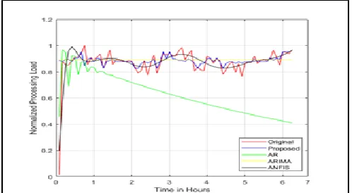
2255 better then AR and ARIMA but still does not performs well
during the peaks. Looking at the proposed algorithm accurately follows the original data even at the variations and peaks. The figure 9(a) and (b), shows the comparison of RMSE values for all four algorithms. From figures it can be noticed that proposed algorithm has the lower RMSE value outperforms the ANFIS by 30% of margin for processing load forecasting and by 125% for memory demand forecasting.
The figure 10(a) and (b), shows the comparison of MAE values for all four algorithms. The proposed algorithm again outperforms all other algorithm with margins similar to those of RMSE.
In this work all performance measures indicates the better forecasting capability of the proposed algorithm in comparison of other state of art algorithms. These results validates the performance of the proposed algorithm.
7 CONCLUSION
In this paper, a fuzzy time series and PSO based cloud load forecasting algorithm is presented. The proposed algorithm uses the PSO to estimate the segment lengths and weights of fuzzy variables. To validate the performance of the proposed algorithm the real data workload data from Google Cloud Traces has been used, and the results are compared with four state of art algorithms in terms of RMSE, MAE, and MAPE. The comparison shows that proposed algorithm improves the RMSE and MAE measures by 30% and MAPE measure by 5 to 10 times which is enormous improvement. Hence the algorithm can be used with cloud manager for accurate workload forecasting. With accurate load forecast the cloud manager can properly balance the load and save the significant power and resources by migrating the status of the active VMs.
8
REFERENCES
[1]. Prevost, John J., KranthiManojNagothu, Brian Kelley, and Mo Jamshidi. "Prediction of cloud data center networks loads using stochastic and neural models." In 2011 6th International Conference on System of Systems Engineering, pp. 276-281. IEEE, 2011. [2]. Hilman, Muhammad Hafizhuddin, Maria Alejandra
Rodriguez, and RajkumarBuyya. "Task Runtime Prediction in Scientific Workflows Using an Online Incremental Learning Approach." In 2018 IEEE/ACM 11th International Conference on Utility and Cloud Computing (UCC), pp. 93-102. IEEE, 2018.
[3]. Kovari, Attila, and P. Dukan. "KVM &OpenVZ virtualization based IaaS open source cloud virtualization platforms: OpenNode, Proxmox VE." In 2012 IEEE 10th Jubilee International Symposium on Intelligent Systems and Informatics, pp. 335-339. IEEE, 2012.
[4]. Wieder, Philipp, Joe M. Butler, Wolfgang Theilmann, and RaminYahyapour, eds. Service level agreements for cloud computing. Springer Science & Business Media, 2011.
[5]. Son, Seokho, Gihun Jung, and Sung Chan Jun. "An SLA-based cloud computing that facilitates resource allocation in the distributed data centers of a cloud provider." The Journal of Supercomputing 64, no. 2 (2013): 606-637.
[6]. Albano, Luca, CosimoAnglano, Massimo Canonico, and Marco Guazzone. "Fuzzy-Q & E: Achieving QoS Guarantees and Energy Savings for Cloud Applications with Fuzzy Control." In 2013 International Conference on Cloud and Green Computing, pp. 159-166. IEEE, 2013.
[7]. Hussain, Altaf, Muhammad Aleem, Abid Khan, Muhammad Azhar Iqbal, and Muhammad Arshad Islam. "RALBA: a computation-aware load balancing scheduler for cloud computing." Cluster Computing 21, no. 3 (2018): 1667-1680.
[8]. Yu, Hui-Kuang. "Weighted fuzzy time series models for TAIEX forecasting." Physica A: Statistical Mechanics and its Applications 349, no. 3-4 (2005): 609-624.
[9]. Zhong, Wei, Yi Zhuang, Jian Sun, and JingjingGu. "The cloud computing load forecasting algorithm based on wavelet support vector machine." In Proceedings of the Australasian Computer Science Week Multiconference, p. 38. ACM, 2017.
[10]. Zhong, Wei, Yi Zhuang, Jian Sun, and JingjingGu. "A load prediction model for cloud computing using PSO-based weighted wavelet support vector machine." Applied Intelligence 48, no. 11 (2018): 4072-4083. [11]. Toony, Ahmed A., Mustafa Abdul Salam, and
DiaaSalamaAbd-Elminaam. "Prediction of Host Load in Cloud Computing Based on Quantum Evolutionary
Algorithm and Kalman Filter with
ANFIS." INTERNATIONAL JOURNAL OF COMPUTER SCIENCE AND NETWORK SECURITY 17, no. 9 (2017): 59-64.
[12]. Calheiros, Rodrigo N., EnayatMasoumi, Rajiv Ranjan, and RajkumarBuyya. "Workload prediction using ARIMA model and its impact on cloud applications’ QoS." IEEE Transactions on Cloud Computing 3, no. 4 (2014): 449-458.
[13]. Vazquez, Carlos, Ram Krishnan, and Eugene John. "Time Series Forecasting of Cloud Data Center
Workloads for Dynamic Resource
Provisioning." JoWUA 6, no. 3 (2015): 87-110.
[14]. Kumar, Jitendra, and Ashutosh Kumar Singh. "Workload prediction in cloud using artificial neural network and adaptive differential evolution." Future Generation Computer Systems 81 (2018): 41-52. [15]. Chen, Zhijia, Yuanchang Zhu, Yanqiang Di, and
Shaochong Feng. "Self-adaptive prediction of cloud resource demands using ensemble model and subtractive-fuzzy clustering based fuzzy neural network." Computational intelligence and neuroscience 2015 (2015): 17.
[16]. Yang, Dingyu, Jian Cao, Jiwen Fu, Jie Wang, and JianmeiGuo. "A pattern fusion model for multi-step-ahead CPU load prediction." Journal of Systems and Software 86, no. 5 (2013): 1257-1266.
[17]. Chang, Yao-Chung, Ruay-Shiung Chang, and Feng-Wei Chuang. "A predictive method for workload forecasting in the cloud environment." In Advanced Technologies, Embedded and Multimedia for Human-Centric Computing, pp. 577-585. Springer, Dordrecht, 2014.
[18]. Kawakami, Kazuya. "Supervised sequence labelling with recurrent neural networks." Ph. D. dissertation, PhD thesis. Ph. D. thesis (2008).
[19]. Wang, Hengjian, John Pannereselvam, Lu Liu, Yao Lu, XiaojunZhai, and Haider Ali. "Cloud Workload Analytics for Real-Time Prediction of User Request Patterns." In 2018 IEEE 20th International Conference on High Performance Computing and Communications; IEEE 16th International Conference on Smart City; IEEE 4th International Conference on Data Science and Systems (HPCC/SmartCity/DSS), pp. 1677-1684. IEEE, 2018.
2257 [21]. Song, Qiang, and Brad S. Chissom. "Fuzzy time series
and its models." Fuzzy sets and systems 54, no. 3 (1993): 269-277.
[22]. Chen, Shyi-Ming. "Forecasting enrollments based on fuzzy time series." Fuzzy sets and systems 81, no. 3 (1996): 311-319.
[23]. Eberhart Russell, and James Kennedy. "Particle swarm optimization." In Proceedings of the IEEE international conference on neural networks, vol. 4, pp. 1942-1948. Citeseer, 1995.
[24]. Garcia-Gonzalo, Esperanza, and Juan Luis Fernandez-Martinez. "A brief historical review of particle swarm optimization (PSO)." Journal of Bioinformatics and Intelligent Control 1, no. 1 (2012): 3-16.
[25]. Pluhacek, Michal, Roman Senkerik, Adam Viktorin, Tomas Kadavy, and Ivan Zelinka. "A review of real-world applications of particle swarm optimization algorithm." In International Conference on Advanced Engineering Theory and Applications, pp. 115-122. Springer, Cham, 2017.
[26]. Žerovnik, Janez. "Heuristics for NP-hard optimization problems-simpler is better!?." Logistics & Sustainable Transport 6, no. 1 (2015): 1-10.
[27]. Repository for various traces from parts of the Google cluster management software and systems.
https://github.com/google/cluster-data.
[28]. Hussain, Altaf, and Muhammad Aleem. "GoCJ: Google cloud jobs dataset for distributed and cloud computing infrastructures." Data 3, no. 4 (2018): 38.
[29]. Bhatia, Munish, Sandeep K. Sood, and Simranpreet Kaur. "Quantumized approach of load scheduling in fog
computing environment for IoT
applications." Computing (2020): 1-19.
[30]. Hussain, Altaf, Muhammad Aleem, Muhammad Azhar Iqbal, and Muhammad Arshad Islam. "SLA-RALBA: cost-efficient and resource-aware load balancing algorithm for cloud computing." The Journal of Supercomputing 75, no. 10 (2019): 6777-6803.
[31]. Hussain, Altaf, MuhamamdAleem, Muhammad Arshad Islam, and Muhammad Iqbal. "A rigorous evaluation of state-of-the-art scheduling algorithms for cloud computing." IEEE Access 6 (2018): 75033-75047.
[32]. GoCJ: Google Cloud Jobs Dataset,
https://data.mendeley.com/datasets/b7bp6xhrcd/1
[33]. NASA Kennedy Space Center,NASA-HTTP Traces
from WWW server in Florida.,
file:///C:/Users/admin/Downloads/NASA-HTTP.html
[34]. Google Cluster Dataset,