© 2015 IJSRST | Volume 1 | Issue 2 | Print ISSN: 2395-6011 | Online ISSN: 2395-602X Themed Section: Science and Technology
Parameters Analysis Characterizing the EFG Meshfree Metod for
Two-Dimensional Elastic Beam Problem
Prof. Sanjaykumar D. Ambaliya
*1, Prof. Ketan D. Panchal
2, Prof. Hemal N. Lakdawala
31
Department of Mechanical Engineering, Government Engineering College, Surat, Gujarat, India 2,3
Department of Mechanical Engineering, Government Engineering College, Valsad, Gujarat
ABSTRACT
The Finite Element Method (FEM) is well established for modelling complex problems for engineering problems in various fields. However, the difficulty of meshing and remeshing of complex structural elements in several classes of problems is the main drawback that FEM possess. To prevent this drawback, Mesh Free numerical techniques have been developed in such a way that the mesh is not more necessary to discretize the problem, and the trial functions are constructed entirely in terms of a set of nodes without the necessity of element descretization for the construction of the equations. Element Free Galerkin method (EFG) is one of the most interesting meshless methods which is based on global weak form of governing differential equation and employs Moving Least Square (MLS) approximants to construct shape functions. To implement this technique, it is necessary to characterize the significant parameters like, order of monomial basis function, weight function selection in MLS approximants, the size of influence domain, uniform and non-uniform node distribution, number of Gauss points in integration cells. In this paper, the EFG method has been extended to solve elasto-static beam problem in plane stress cases for node distribution scheme, number of Gauss points in integration cells. For implementation and solution, a MATLAB program has been developed to verify the accuracy of the proposed meshless method and results are compared with exact analytical solutions.
Keywords: EFG, MLS Shape Functions, Weight Functions, Meshfree, Matlab, Monomial Basis, Size Of Influence Domain.
I.
INTRODUCTION
The Finite Element Method (FEM) has been well established and used widely in many branches of engineering. However, it still has some shortcomings. The reliance of the FEM method on a mesh leads to complications for certain classes of problems due to considerable loss in accuracy arises due to element distortion. The modelling of large deformation processes, examining the growth of cracks with arbitrary and complex paths, and the simulations of phase transformations is also difficult with FEM. Many theories of meshless methods were proposed to reduce some of the shortcomings of FEM, such as EFG, MLPG, and PIM, as discussed by Liu [1].
In a meshless method, unlike FEM, a predefined mesh is not necessary, at least in field variables interpolation. In
proposed by Gingold and Monaghan, Meshless Local Petrov-Galerkin (MLPG) method proposed by Atluri, and some other methods [3, 5]. The well-establish EFG method use shape functions which are derived from moving least square (MLS) approximation. In 1981, Lancaster and Salkauskas formulated the Moving Least square approach [Lancaster, 1981]. Nayroles et al (1992) first used it for meshfree approximation and the idea was further formulated into EFGM framework by Belytschko et al (1994). MLS involves the assumption of the field variable as a summation of series of monomials. The coefficients of the monomials are the unknowns and are calculated such that the squared sum of errors in the domain of a point is minimal. Once the approximation at a point is over, the MLS is „moved‟ to another point.
This paper characterize the significant selectable parameters like, node distribution scheme, and number of points in gauss integration for EFG method by the results obtained with the simulation of Timoshenko‟s beam through graphical output of the displacement fields and of normal and shear stress fields.
II.
METHODS AND MATERIAL
2.1 System of Equation:
Consider a displacement function u(x) of a field variable defined on the domain Ω, the MLS approximant
u
ˆ
(x)of the function u(x) can be represented as,Where, PT (x) is monomial basis functions of order m and a(x) are vector coefficients.
For 2-D problems,
PT(x) = [1, x, y] Linear, m=3 and
0 1 2
( )
[
( )
( )
( ) ,...
( )]
T
m
a
x
a x
a x
a x
a
x
The unknown parameters a(x) at any given point are determined by minimizing the difference between the local approximation at that point and the nodal parameters ui. Let the nodes whose supports include xbe
given local node numbers 1 to n. In order to determine the unknown coefficients a, a functional J is constructed. It sum up the weighted quadratic error for all nodes inside the support domain as
Where n is the number of nodes in the neighbourhood of
x for which the weight function, W(x — xi) ≠ 0, and ui
refers to the nodal parameter of u at x = xi.
The weights functions like cubic weight function, quartic weight, exponential weight etc, perform two actions, one as a medium of imparting smoothness or desired continuity to the approximation and other one, more important, is the establishment of the local nature of the approximation. The polynomial basis and the weight function together cast a major influence on the performance of the MLS method.
We want to minimize this functional, so we differentiate with respect to the unknown vector a(x), containing the coefficient,
J
a
= 0
Which results in the following compact matrix form as,
( ) ( )
( )
A x a x
B x u
1
( )
( ) ( )
a x
A
x B x u
Where,
1 1 1
1
(
) ( )
( )
n
T I
A
w x
x P x P
x
[
1, 2,... ]
T
n
u
u u
u
By inserting this expression, we get a new formulation of the displacement field,
1
( )
ˆ
T( ) ( )
T( )
( ) ( ) ( )
x
u
P x a x
P x A
x B x U x
= 1 ( ) ( ) n i i iu x
x u
Where, the shape function is defined by,
1 1 1
( )
( )(
( ) ( ))
n TI I I
i
x
P x A
x B x
p A B
2.2 Discrete equations in two-dimensional problems:
The partial differential equation for two-dimensional problem on the domain , bounded by
can be written as:0
b in
Where
is stress tensor, which corresponds to the displacement field u and b is a body force vector. The boundary conditions are given as follows:n
n
t
on
t
u
u
u
on
In which the superposed bar denotes prescribed boundary values, and n is the unit normal to the domain .The Weak form of the equilibrium equation is posed as follows, consider trial functions u(x)ε H1
and Lagrange multipliers λ ε H0, test functions δv(x)ε H0, [2]
1 0
( ) : ( ) ,
t u u
T T T T T
sv d v bd v td u u d v d v H H
Which yield, the following system of linear algebraic equations:
0
T
K G U F
G
q Where, T
IJ I J
K
B DB d
IK u t K
G N d
t t t t
f
td
td
u
k k
q N ud
, , , , 0 0 I xt I y
I y I x
2
1
0
1
0
1
(1
)
0
0
2
v
E
D
v
v
v
In which, Kis the stiffness matrix, G is the boundary condition matrix, u is the nodal displacements vector, λ is the Lagrange multipliers, f is the force vector and q is a boundary condition vector, E is Young's modulus and v is Poisson‟s ratio, respectively.
3. NUMERICAL EXAMPLES
In this section, a plane stress Timoshenko beam problem is solved using an EFG program written in MATLAB. This example serves to illustrate the accuracy of the EFG method by comparing it to the exact solution [2, 4].
Figure 1 : Timoshenko Beam
Consider a beam of length L = 48 unit subjected to parabolic traction at the free end as shown in figure. The beam has characteristics height D=12 unit and is considered to be of unit depth and is assumed to be in a state of plane stress with P= 1000 unit, v = 0.3 and E= 3.0 x 10⁷.
The exact analytical solution of Timoshenko beam is given by the following equations [1, 2]. The expressions for displacements in x direction, ux, and in y direction, uy, are respectively:
III.
RESULT AND DISCUSSION
5. Numerical Results
The solutions were obtained using a linear basis function with cubic spline weight function and dmax value of 3.5. The stress values along different section are plotted and comparative performance is evaluated for different node distribution and gauss integration methods.
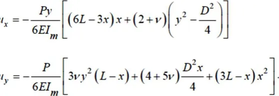
Figure 2. Node Distribution
Figure 3. Background Cell
Figure 4. Gauss Points
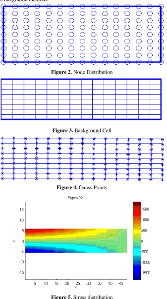
Figure 6. Displacement for EFG and Exact
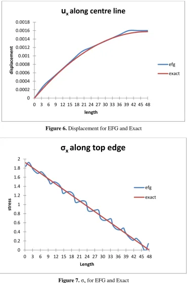
Figure 7. σx for EFG and Exact 0
0.0002 0.0004 0.0006 0.0008 0.001 0.0012 0.0014 0.0016 0.0018
0 3 6 9 12 15 18 21 24 27 30 33 36 39 42 45 48
d
isp
lac
e
m
e
n
t
length
u
xalong centre line
efg
exact
0 0.2 0.4 0.6 0.8 1 1.2 1.4 1.6 1.8 2
0 3 6 9 12 15 18 21 24 27 30 33 36 39 42 45 48
st
re
ss
Length
σ
x
along top edge
efg
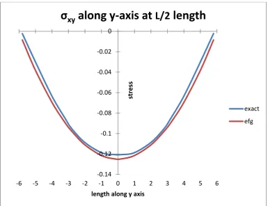
Figure 8.
σ
xyfor EFG and Exact
Table 1: Comparative study for 2 D Beam
Results of stress σ
xat point (24,-6) for 11x7 node distribution
Gauss point
σ
efgσ
exact%error
4x4
937.63
1000
6.237
5x5
940.6
1000
5.94
6x6
945.38
1000
5.462
7x7
950.32
1000
4.968
Results of displacement u
yat point (48,6) for 4x4 gauss point
Node
distribution
U
efgu
exact%error
6x4
-0.00802
-0.0089
9.88764
11x7
-0.00874
-0.0089
1.797753
20x8
-0.00889
-0.0089
0.11236
21x10
-0.00889
-0.0089
0.11236
IV.
CONCLUSION
For 2D Timoshenko beam problem it has been found that the accuracy of the EFG is directly proportional to the number or nodes. With the increase in the number of nodes the accuracy of the EFGM automatically increases. Similarly, keeping the number of nodes
constant, we can increase the quadrature points to decrease the error value.
-0.14 -0.12 -0.1 -0.08 -0.06 -0.04 -0.02 0
-6 -5 -4 -3 -2 -1 0 1 2 3 4 5 6
st
re
ss
length along y axis
σ
xy
along y-axis at L/2 length
exact
V.
REFERENCES
[1]. Liu G. R., 2004, “Mesh Free Methods: moving beyond the finite element method”, Ed. CRC Press, Florida,USA,
[2]. T. Belytschk O, Y.Y.Lu And L.GU, "An Introduction to Programming the Meshless Element Free Galerkin Method" International journal for numerical methods in engineering, VOL. 37, 121-256 (1994).
[3]. T. Belytschko,Y. Krongauz, D. Organ, "Meshless Methods: An Overview and Recent Developments" May 2, 1996.
[4]. J. Dolbow, T. Belytschko, "Numerical integration of the Galerkin weak form in meshfree methods" Computational Mechanics 23 (1999) 219-230 Ó Springer-Verlag 1999.
[5]. S. D. Daxini and J. M. Prajapati, "A Review on Recent Contribution of Meshfree Methods to Structure and Fracture Mechanics Applications" Scientific World Journal Volume 2014, Article ID 247172, 13 pages
[6]. "An Introduction to Meshfree methods and their Programming" by G.R. LIU, 2005.
[7]. "From Weighted Residual Methods to Finite
Element Methods" by Lars‐Erik Lindgren, 2009. [8]. "Meshfree and Generalized Finite Element
Methods" by Habilitationsschrift, 2008