An Algorithm to Define the Node Probability
Functions of Bayesian Networks based on Ranked
Nodes
Joa˜o Nunes
∗1, Renan Willamy
†1, Mirko Perkusich
‡2, Renata Saraiva
§2, Kyller Gorgonio
¶2, Hyggo Almeida
2, and
Angelo Perkusich
∗∗21
Federal University of Campina Grande, Campina Grande, Brazil 2
Embedded and Pervasive Computing Laboratory, Federal University of Campina Grande, Campina Grande, Brazil
Abstract
Bayesian Network (BN) has been used in a broad range of applications. A challenge in constructing a BN is defining the node probability tables (NPTs), which can be learned from data or elicited from domain experts. In practice, it is common to not have enough data for learning and elicitation from experts is the only option. However, the complexity of defining NPTs grows exponentially, making their elicitation process costly and error-prone. Previous work proposed a solution: the ranked nodes method (RNM). However, the details necessary to implement it were not presented. Nowadays, the solution is only available through a commercial tool. Hence, this paper presents an algorithm to define NPT using the RNM. We include details regarding sampling and how to mix truncated Normal distributions and convert the resulting distribution into an NPT. We compared the results calculated using our algorithm with the commercial tool through an experiment. The results show that our solution is equivalent to the commercial tools’ in terms of NPT definition with a mean difference of 1.6%. Furthermore, our solution is faster. The solution developed is made available as open source software.
Bayesian Network; Expert systems; Node Probability Table; Ranked nodes
1
Introduction
Bayesian Network (BN) is a mathematical model that graphically and numerically represents the probabilistic relationships between random variables through Bayes theorem. Recently, given the evolution of the computational capacity, which enabled the calculation of complex BNs, it has become a popular technique to assist on decision- making [7]. It has been applied in several areas such as large-scale engineering projects [11], software engineering [14, 13], and sports management [3].
However, constructing a BN is challenging and this problem can be subdivided into: (i) building the directed acyclic graph (DAG) and (ii) defining the NPTs. In this research, we focus on (ii). In cases in which there is a database with enough information for the given domain, it is possible to automate the process of defining the NPT through batch learning [9]. Unfortunately, in practice, in most cases, there is not enough data [7]. Furthermore, experts can often understand and identify key relationships that data alone may fail to discover [2]. Therefore, the concept of smart-data is defined by Constantinou and Fenton [2]: a method that supports data engineering and knowledge engineering approaches with emphasis on applying causal knowledge and real-world facts to develop models. In this context, it is necessary to manually elicit data from domain experts to define the NPTs. Given that the complexity of building NPTs grows exponentially, depending on the number of parents and states, the manual definition of the NPT becomes unfeasible.
RELATIVES HAD
CANCER SMOKE
LUNG CANCER
limited to nodes (i.e., random variables) with an ordinal scale (e.g., Good, Medium, Bad), which are called ranked nodes. In ranked nodes, the ordinal scale is mapped into a scale monotonically ordered in the interval [0, 1]. The solution is based on a Normal distribution truncated between [0, 1] (i.e., TNormal) to represent the NPTs. Given
dependencies between these variables. Θ represents the set of the probability functions. This set contains the parameter θxi|πi
= PB (xi|πi) for each xi in Xi conditioned by πi, the set of the parameters of Xi in G. Equation 1 presents the joint distribution defined by B over V .
this, the NPT of a child node is calculated as the mixture of n n
the TNormal of its parent nodes. There are four functions to PB (X1, . . . , Xn) = n PB (xi|πi) = n θX i|πi (1) model the mixture: weighted mean (WMEAN), weighted
minimum (WMIN), weighted maximum (WMAX) and i=1 i=1
the mixture of classic minimum and maximum functions (MIXMINMAX). We present more details regarding this approach in Section 3. Currently, this solution is only made available through AgenaRisk1, a commercial tool to construct Bayesian networks.
On the other hand, Fenton et al. [7] do not present the details to, in practice, implement the solution. Despite presenting the mixture functions, there is no information regarding the algorithms used to generate and mix TNormal, define samples size and define a conventional NPT given the calculated TNormals. The last factor enables the integration of ranked nodes with other types of nodes such as boolean and continuous, which brings more modeling flexibility.
In this paper, we present an algorithm to define a NPT for ranked nodes using the functions WMEAN, WMIN and WMAX. For this purpose, we implemented the code in C++ and executed experiments to compare our solution in terms of accuracy and performance with AgenaRisk. The results show that our solution is equivalent to the commercial tools’ in terms of NPT definition within a margin of error of 10%. Furthermore, our solution presented better performance than the existing available commercial tool. The solution is made available in a popular open source website2.
This paper is organized as follows. Section 2 presents an overview on Bayesian networks. Section 3 presents details regarding ranked nodes. Section 4 presents the details of the algorithm developed to implement ranked nodes. Section 5 presents the results of the comparison between our solution and AgenaRisk. Section 6 presents our conclusions, limitations and future works.
2
Bayesian networks
BNs are probabilistic graph models used to represent knowledge about an uncertain domain [1]. A BN, B, is a directed acyclic graph that represents a joint probability distribution over a set of random variables V [8]. The network is defined by the pair B = {G, Θ}. G is the directed acyclic graph in which the nodes X1, . . . , Xn represent random variables and the arcs represent the direct
1www.agenarisk.com
2https://github.com/lockenunes/kaizenbase
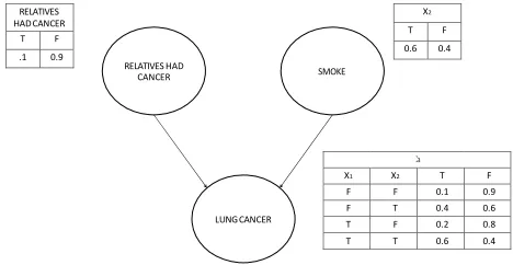
We present an example of a BN in Figure 1, in which ellipses represent the nodes and arrows represent the arcs. The probability functions are usually represented by tables. Even though the arcs represent the causal connection’s direction between the variables, information can propagate in any direction [12].
X 3 X1 X2 T F F F 0.1 0.9 F T 0.4 0.6 T F 0.2 0.8 T T 0.6 0.4
Figure 1. A Bayesian network example.
3
Related works
The problem of defining NPT for large-scale Bayesian networks has already been discussed in the literature. There are several methods to reduce the complexity and to encode expertise in large node probability tables. For instance, Noisy-OR [10] and Noise-MAX [5] are well-established methods, but Noisy-OR only applies to Boolean nodes, and Noisy-MAX does not model the range of relationships we need. Furthermore, Das [4] presented the Weighted Sum Algorithm (WSA), a solution to semi-automatically define NPTs through knowledge elicited from domain experts.
In Fenton et al. [7], an approach similar to WSA was proposed: the Ranked Nodes Method (RNM). A ranked node is a random variable represented in an ordinal scale monotonically ordered in the interval [0, 1]. For instance, for the ordinal scale [“Bad”, “Moderate”, “Good”], Bad is represented by the interval [0, 1/3]; Moderate, by [1/3,
2/3]; and Good, by [2/3, 1]. This concept is based on the doubly truncated Normal distribution (TNormal) limited in the
[0, 1] region. This distribution is based on four
X2
T F 0.6 0.4 RELATIVES
WMEAN WMIN
WMAX MIXMINMAX
Figure 2. TNormal examples.
parameters: µ, mean (i.e., central tendency); σ2, variance (i.e., confidence in the results); a, lower bound (i.e., 0); and, b, upper bound (i.e., 1). This distribution enables us to model a variety of shapes (i.e., relationships) such as a uniform distribution, achieved when σ2 = ∞, and highly skewed distributions, achieved when σ2 = 0. In Figure 3, we show an example of TNormal with same µ, but different σ2.
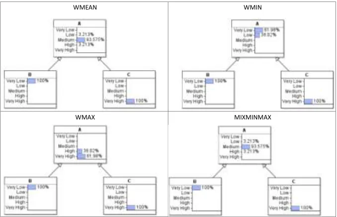
between the two functions is that WMEAN calculates the weighted mean of the parent node’s values (i.e., the weights are set for the parent nodes) and MIXMINMAX mixes the minimum and maximum functions (i.e., the weights are set for the functions, instead of the parents).
We chose to implement the RNM approach due to its popularity given the number of referrals and its conceptual potential to be more flexible. In Fenton et al. [7], as already mentioned, four functions were presented to combine the data of the parent nodes into the child. On the other hand, more functions could be defined, if necessary. We
µ = 0.5
σ 2 = 1
µ = 0.5
σ 2 = 0.01
complement the work of Fenton et al. [7] by presenting all the steps required to implement ranked nodes and making the source code available to the community.
4
Details of the algorithm
Figure 3. Examples of TNormal.
µ is defined by a weighted function of the parent nodes. Fenton et al. [7] present four functions: weighted mean (WMEAN), weighted minimum (WMIN), weighted maximum (WMAX) and a mixture of classic minimum and maximum functions (MIXMINMAX). According to the authors, these functions are enough to represent the types of relationship necessary to define NPTs. We show examples of NPTs calculated with these functions in Figure 2. In the examples presented in Figure 2, WMEAN and MIXMINMAX have the same values. The difference
The algorithm is probabilistic and composed of two main steps: (i) generate samples for the parent nodes and (ii) construct the NPT. In step (ii), for each possible combination of values for the parent nodes (i.e., each column of the NPT), the samples defined in the previous step are mixed given a function selected by the user and a TNormal is generated using the resulting mix and a variance defined by the user. An overview of the algorithm is shown in Figure 4.
Figure 4. Overview of the algorithm.
U (0, 1/3) ∪ pmoderate ∗ U (1/3, 2/3) ∪ pgood ∗ U (2/3, 1), where p is the density of the distribution. For the example shown in Figure 5, the set of uniform distributions is composed of the union of three uniform distributions: U (0, 1) = 54.7 ∗ U (0, 1/3) ∪ 36.5 ∗ U (1/3, 2/3) ∪ 8.80 ∗
U (2/3, 1). Numerically, this union is calculated using samples. Considering a sample size of 10,000, to represent the NPT shown in Figure 5, it is necessary to collect 5,
700 random samples from U (0, 1/3), 3, 650 random samples from U (1/3, 2/3) and 880 random samples from U (2/3, 1).
Figure 4 shows that the algorithm is composed of four collections: repository[], a vector to store the samples of base states for the parent nodes; parents[k], a vector to store references to the parent nodes of each child node, in which k is the number of parents; states[m], a vector to store the states of each node, in which m is the number of possible values for the child node given the combination of its parents states; and distribution[m], a vector to store the resulting distribution for each possible combination of states of the parent nodes.
We used the repository strategy for optimization purposes. First, we register in memory (i.e., in repository[]) distributions that represent the base states, which are states with an evidence (i.e., a node has 100% of chance for a
samples of a uniform distribution limited in the interval [2/3,
1]. Empirically, we defined that using a sample size of 10,000 is enough to guarantee a margin of error less than 0.1%. We registered each sample with meta-data regarding its configuration (i.e., number of states and µ).
We used the data in repository[] to generate samples for a node. Therefore, the samples for a base state are only generated once and reused later. This step is represented in Figure 4 by the block Generation of samples.
The next step consists of, for each combination of the parent nodes, mix the TNormal using equidistant samples, randomly selected, for each parent node. Empirically, we defined that 10,000 equidistant samples is enough to guarantee a margin of error less than 0.1. The samples are mixed using a given function (e.g., WMEAN, WMIN, WMAX or MIXMINMAX) and the defined variance.
To mix the distributions, we, randomly, remove an element from each sample of the parents and use them to calculate a resulting element using a given function. For instance, consider node A with two parents B and C. If we are calculating the probabilities of A for the combination Low-High and the selected function is WMEAN with equal weights, if the values removed in an iteration were 0.1 and 0.7, the resulting value would be 0.4. This step must be repeated until the
collections of samples are empty. 2
given state). For instance, for a node composed of the states [Bad, Moderate, Good], we registered the samples for: 100% Bad, 100% Moderate and 100% Good, which respectively has µ = 1/6, µ = 1/2 and µ = 5/6. For this purpose, we collected samples from a uniform distribution with the limits defined given the thresholds of the scale. For instance, for 100% Good, we collected
Afterwards, the set of calculated elements and the given σ are used as input to generate a TNormal. With this purpose, we used the library TRUNCATED NORMAL3.
The resulting distribution is converted to an ordinal scale and represents a column in the NPT of the child node (i.e.,
3http://people.sc.fsu.edu/ jburkardt/cpp src/
AgenaRisk C++
µ σ2 µ σ2 Percentage difference (%)
0.1 0.007 0.3 0.0842 0.9
0.3 0.15 0.3 0.39 0.3
0.5 0.15 0.5 0.39 0.4
0.8 0.15 0.8 0.39 0.9
0.9 0.007 0.5 0.0842 0.5
Table 1. Results for generating one node with WMEAN.
Low
AgenaRisk’s.
On the other hand, to compare the solutions, we defined some tests cases and empirically calibrated σ2 to have equivalent values for both algorithms (i.e., not necessarily the same). Given that the calibration was manual, there is no guarantee that we found the best values σ2. For instance, for the configuration D =
A + B + C, we found that the results are equivalent if σ2 = 0.0005 in AgenaRisk and
0 1/3 2/3 1
Figure 5. Conversion from ordinal to
continuous scale.
in the given example, the column for the combination Low- High). At the end of this step, all the possible combinations of states of the parent node are evaluated and the NPT for the child node is completed.
5
Validation
We implemented the algorithm presented in Section 4 in C++. We chose this language, due to its efficiency, to use the library TRUNCATED NORMAL and to facilitate the integration with SMILE4, which is a library of C++ for reasoning in graphical probabilistic models. To validate our solution, we defined test cases and compared our results with AgenaRisk’s.
Conceptually, our solution is correct if it is as flexible as AgenaRisk to generate curves. Since calibration is a natural step in creating BNs, having the same inputs (i.e., ) generating different result is not an issue. Assuming that the equations presented in Fenton et al. [7] are correct and that library TRUNCATED NORMAL generates proper truncated Normal distributions, there is no reason to conclude that our approach is not equivalent to
4https://dslpitt.org/genie/wiki/SMILE Documentation
State Probability
Low 54,7
Moderate 36,5
High 8,80
54,7%
Moderate
36,5%
High
σ2 = 0.075 in TRUNCATED NORMAL.
Given that it is recommended to improve the graph of the BN if a given node has more than three parents [6], we only evaluated our approach with two structures: a single node (i.e., most simple) and a node with three parents (i.e., most complex). For the single node case, we randomly defined a µ and σ2 for AgenaRisk and ran 10 tests with WMEAN. For WMEAN, the mean difference between AgenaRisk and our solution for independent nodes was 0.6%, as shown in Table 1.
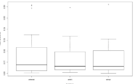
For the case with three parent nodes, we evaluated four structures for each function. The mean difference of the results was 1.6%, with the worst case being 6.2%. In Figure 6, we show the box plot for the results for each function.
Regarding performance, our solution was faster. For a BN composed of a child node with three parents, in average, AgenaRisk executed in 1.92 seconds; in our solution, it executed in 0.34 seconds. Given that the standard deviations were less than 0.1, it is clear that our solution is faster. Therefore, we did not perform hypothesis testing. On the other hand, it is necessary to consider that our solution is dedicated only to defining NPT and AgenaRisk is a more robust tool with a graphical user interface and several features.
6
Conclusions
Despite recent popularity, the construction of BNs is still challenging. One of the challenges refers to defining the NPTs for large-scale BN. It is possible to automate this process using batch learning, but it requires a database with enough information. In practice, this is not common. The other option is to elicit data from experts, which is unfeasible if it is required to manually define the probabilities of all combinations of the states of the parent nodes. Fenton et al. [7] presented a solution based on ranked nodes, but it lacks the necessary steps to apply it in practice without AgenaRisk, which is a commercial tool. In this paper, we complement the work of Fenton et al. [7] by presenting an algorithm to implement ranked nodes with details regarding sample size for the probability distributions and how to define a conventional NPT given the calculated TNormals. We compared our results with AgenaRisk and achieved acceptable results. In our experiments, our solution reached a mean difference of
1.6%. Given our analysis, we concluded that differences between our solution and AgenaRisk are because of the different implementations of TNormal used as base by the algorithms. This solution is currently limited to WMEAN, WMAX and WMIN.
For future works, we will implement the MIXMINMAX function. Furthermore, we will implement an algorithm to automate the calibration of the NPTs based on data elicited by the domain expert.
References
[1] I. Ben-Gal. Bayesian Networks. John Wiley and Sons, 2007.
[2] A. Constantinou and N. Fenton. Towards smart-data: Improving predictive accuracy in long-term football team performance.
Knowledge-Based Systems, pages –, 2017.
[3] A. C. Constantinou, N. E. Fenton, and M. Neil. Profiting from an inefficient association football
gambling market: Prediction, risk and uncertainty using bayesian networks. Knowledge-Based Systems, 50:60 – 86, 2013.
[4] B. Das. Generating Conditional Probabilities for Bayesian Networks: Easing the Knowledge Acquisition Problem.
Computing Research
Repository, cs.AI/0411034, 2004.
[5] F. J. Diez. Parameter adjustment in bayes networks. the generalized noisy or-gate. In Proceedings of the 9th Conference on
Uncertainty in Artificial Intelligence, pages 99–105. Morgan
Kaufmann, 1993.
[6] N. Fenton and M. Neil. Risk Assessment and Decision Analysis with
Bayesian Networks. CRC Press, 5 edition, 11 2012.
[7] N. E. Fenton, M. Neil, and J. G. Caballero. Using ranked nodes to model qualitative judgments in bayesian networks. IEEE Trans. on
Knowl. and Data Eng., 19(10):1420–1432, Oct. 2007.
[8] N. Friedman, D. Geiger, and M. Goldszmidt. Bayesian network classifiers. Machine Learning, 29(2-3):131– 163, 1997.
[9] D. Heckerman. Learning in graphical models. chapter A Tutorial on Learning with Bayesian Networks, pages 301–354. MIT Press, Cambridge, MA, USA, 1999.
[10] K. Huang and M. Henrion. Efficient search-based inference for noisy-or belief netwnoisy-orks: Topepsilon. In Proceedings of the Twelfth
International Conference on Uncertainty in Artificial Intelligence,
UAI’96, pages 325–331, San Francisco, CA, USA, 1996. Morgan Kaufmann Publishers Inc.
[11] E. Lee, Y. Park, and J. G. Shin. Large engineering project risk management using a bayesian belief network. Expert Syst. Appl., 36(3):5880–5887, Apr. 2009.
[12] J. Pearl and S. Russell. Bayesian networks. Handbook of brain theory and
neural networks, 1995.
[13] M. Perkusich, K. Gorgonio, H. Almeida, and
A. Perkusich. Assisting the continuous improvement of scrum projects using metrics and bayesian networks. Journal of Software: Evolution and Process, 2016. Article in Press.
[14] M. Perkusich, G. Soares, H. Almeida, and A. Perkusich. A procedure to detect problems of processes in software development projects using bayesian networks. Expert