Species and Ecosystems Stages of Biodiversity Evaluation Using Remotely-Sensed Data

(1)

Species and Ecosystems Stages of Biodiversity Evaluation Using

Remotely-Sensed Data

Azniv Petrosyan1

Abstract

Knowledge of historical variations in landscapes offers helpful insights into present species and ecosystems biodiversity stages and supports future strategies on management, decision and conservation. The covers and arrangements of constant vegetation patches are important indicators of keeping resources. Patchiness attributes, as descriptors of resource preservation potentials in landscapes, can be obtained from the remotely-sensed imagery. The objective of this study is to assess land use change and the related biodiversity variations in the landscape of Attica, Greece. Remotely sensed images are geo-corrected and introduced in the image processing software packages. Representative indicators regarding the species (sparse vegetation - α diversity, medium vegetation - β diversity, dense vegetation - γ diversity) and ecosystems (landscapes - eco-zones) biodiversity stages are picked and measured through selective indices. The purposes of the current paper are to estimate the current status, trends and changes in the preferred indicators of the important landscapes and appraise the geographic coverage and extent of the landscapes' patterns and types.

Keywords: Biodiversity Economics, Environmental Indicators, RS metrics, NDVI,

Landscape Assessment, Species and Ecosystems Stages

1. Introduction

In the last decades, human impacts on the land has increased enormously varying landscapes with imperative environmental consequences such as biodiversity loss, deforestation, soil erosion and desertification.

1_{PhD, Laboratory of Remote Sensing, School of Rural and Surveying Engineering, National Technical}

(2)

In addition, human impacts through agriculture and industry persuade variations in climate and earth capacities (Giordano & Marini, 2008; Tagil, 2007; Greco etc, 2005; Lopez-Bermudez and Garcia Gomez, 2003). Humans impacts escort harmful effects on the sustainable resource usage. The environmental progress supervision of sustainable development requires indicators on natural status (Hall, 2001). Environmental indicators with the augment of scientific understanding and educated employment express sustainable use of natural resources. ANZECC (2000) presents 75 indicators mainly with the use of remote sensing.

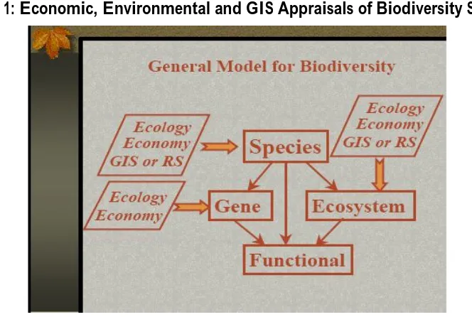
A key aspect in the examination of Biodiversity is the description of the phrase “biodiversity”. Turner etc. (1999) points up that biodiversity economics comprises four stages as: Genes, Species, Ecosystems and Functions. Afterwards, there is given a new approach to the biodiversity of economics. Four stages of Biodiversity have three ways of assessments, i.e. Economic (U.S. Environmental Protection Agency, 2002), Environmental (Peter etc, 2008) and GIS (Strand etc, 2007) appraisals of Biodiversity as implemented by Petrosyan (2010) in Figure 1. Making parallel in Fischer & Lindenmayer (2007), Foley etc (2005), Fazey etc (2005), Foody (2003), Jensen (2000) and Turner etc (1999) characterizations, two stages of biodiversity can be portrayed as:

 Species = Classes = Biodiversity = Habitats: o _{α diversity;}

o _{β diversity;} o _{γ diversity;}

(3)

Figure 1: Economic, Environmental and GIS Appraisals of Biodiversity Stages

Source: Petrosyan (2010)

(4)

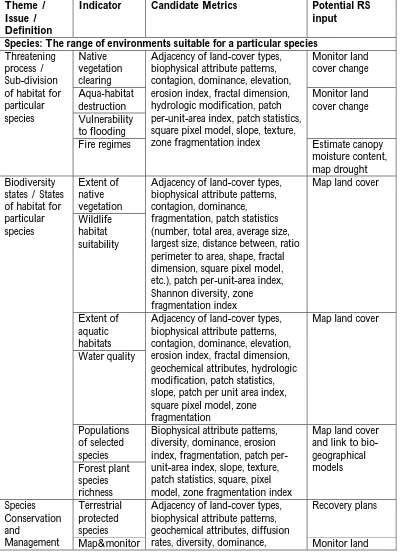
Table 1. Themes, Issues, Definitions of Species and Ecosystems Biodiversity Stages as Per Candidate Metrics Using RS Inputs

Theme / Issue / Definition

Indicator Candidate Metrics Potential RS

input

Species: The range of environments suitable for a particular species

Threatening process / Sub-division of habitat for particular species

Native vegetation clearing

Adjacency of land-cover types, biophysical attribute patterns, contagion, dominance, elevation, erosion index, fractal dimension, hydrologic modification, patch per-unit-area index, patch statistics, square pixel model, slope, texture, zone fragmentation index

Monitor land cover change

Aqua-habitat destruction

Monitor land cover change Vulnerability

to flooding

Fire regimes Estimate canopy

moisture content, map drought Biodiversity

states / States of habitat for particular species

Extent of native vegetation

Adjacency of land-cover types, biophysical attribute patterns, contagion, dominance, fragmentation, patch statistics (number, total area, average size, largest size, distance between, ratio perimeter to area, shape, fractal dimension, square pixel model, etc.), patch per-unit-area index, Shannon diversity, zone fragmentation index

Map land cover

Wildlife habitat suitability

Extent of aquatic habitats

Adjacency of land-cover types, biophysical attribute patterns, contagion, dominance, elevation, erosion index, fractal dimension, geochemical attributes, hydrologic modification, patch statistics, slope, patch per unit area index, square pixel model, zone fragmentation

Map land cover

Water quality

Populations of selected species

Biophysical attribute patterns, diversity, dominance, erosion index, fragmentation, patch per-unit-area index, slope, texture, patch statistics, square, pixel model, zone fragmentation index

Map land cover and link to bio-geographical models Forest plant

species richness Species

Conservation and

Management

Terrestrial protected species

Adjacency of land-cover types, biophysical attribute patterns, geochemical attributes, diffusion rates, diversity, dominance,

Recovery plans

(5)

Theme / Issue / Definition

Indicator Candidate Metrics Potential RS

input

/

The range of environments suitable for particular species

land cover elevation, erosion index,

fragmentation, patch per-unit-area index, slope, percolation threshold, square pixel model, texture, zone fragmentation index

cover, estimate biophysical variables Stream of bio

conditions Area revegetated

Monitor land cover

Ecosystems: A human-defined area ranging

Use and management / A human perspective of land-cover types and environmental gradients in a landscape

Changes in land use

Adjacency of land-cover types diversity, biophysical attribute patterns, diffusion rates, dominance, elevation, erosion index, fragmentation, geochemical attributes, patch per-unit-area index, patch statistics, percolation threshold, Shannon diversity, slope, square pixel model, texture, zone fragmentation index

Monitor land cover

Erosion / Characterized landscape by strong contrast in vegetation patches and surrounding matrix

Potential for erosion

Adjacency of land-cover types, biophysical attribute patterns, contagion, dominance, elevation, erosion index, fractal dimension, hydrologic modification, patch per-unit-area index, patch statistics, slope, square pixel model, texture, zone fragmentation index

Map land cover, link to

environmental data

Landscape Preservation &Management / Range of natures apt as landscape preservation

Earthly protected areas

Biophysical attribute patterns, contagion, dominance,

fragmentation, fractal dimension, patch per-unit-area index, patch statistics, square pixel model, zone fragmentation index

Recovery plans on landscape stage

Landscape sustainability

(6)

In this paper, an investigation of the usefulness of spatial techniques like Remote Sensing and GIS are performed to assess land use changes and the related biodiversity variations. NDVI is calculated to assess vegetation changes for the time period of three (3) continues years during the period of 1984-2002 years. Classification into three (3) classes is performed correspondingly. Landscape metrics are computed to pilot vegetation states as per species and ecosystems biodiversity stages.

2. Materials and Methods

2.1. Study Area

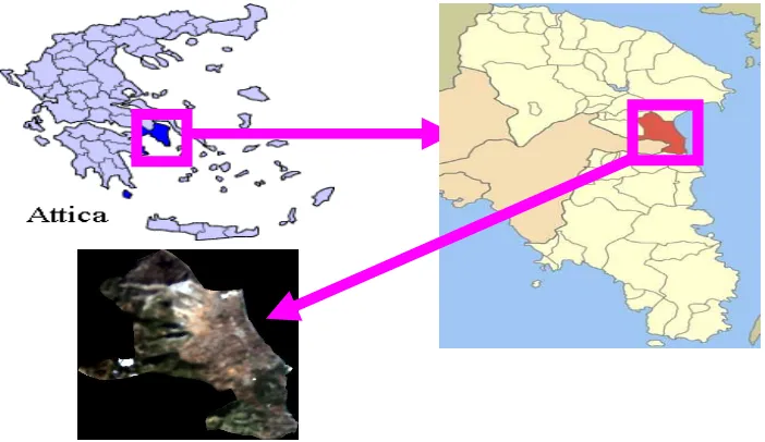
The city of Neas Makris in Figure 2 is located in the northeastern part of Attica of Greece. The area was known as Plesti, which was renamed as Neas Makris because many Greeks moved there after Greek military disaster in Asia Minor. The majority of the population was rural till 1970s. As housing developments arrives to the area, the population approaches to be established. According to Greek statistics captured from national statistical service of Greece (2001) and from Wikipedia (free encyclopedia), the population of Neas Makris is 14,809, the area is 36.662 km² and the density is 404 /km².

(7)

Figure 2: Neas Makris, Attica, Greece

General and specific records affecting to the Municipality of Neas Makris are the followings (Kosioni-Koen and Papastergiou-Mitsopoulou, 2004):

 Nomination and protection of historical data for the landscapes of Athens;  Environmental pollution reduction;

 Implementation of political residence;

 Incorporation of shaped areas for the urban planning;  Flood and earthquake prevention;

 Reconstruction of neighborhoods, interception of flooring, improvement of town, control of treatments and densities;

 Redistribution, operation and organization of development for the urban planning;

 Qualitative interferences of big scaling;

 Supports to the developments of the secondarily urban centers;

 Formation of recreated systems, such as big towns and nets connecting green lands, archeological areas, coastlines, sidewalks and cyclists;

 Survey of Olympic hospitalities in all camps of Agia Andrea and Neas Makris;  Survey of Olympic works in Marathona and North of Neas Makris;

(8)

 Construction of new big roads, railways and train lines with the length of Athens roads and Stavro-Rafinas highways.

2.2. Data Sets

Five (5) Landsat Thematic Mapper (TM) and two (2) Landsat Enhanced Thematic Mapper Plus (ETM+) satellite images are used in the current paper. The whole information for seven (7) satellite images is shown in Table 2.

Table 2: RS Data Used

2.3. Methodology

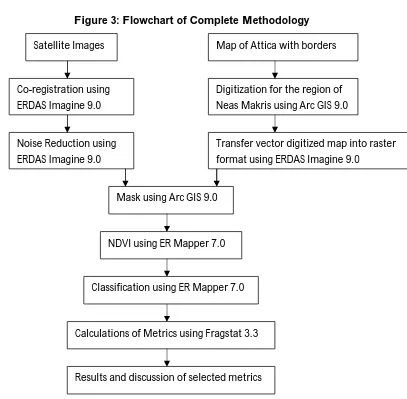
The active occurrence perceptive requires analysis of the land use change. The related biodiversity variations are identified and computed through landscape metrics. Erdas (Leica) (ERDAS, 2005, 1997), ArcGIS software ESRI (Koutsopoulos and Androulakis, 2005; ESRI, 1997, 1994), ER Mapper (ER MAPPER, 2005) and Fragstat (McGarigal and Marks, 1995) software are used to analyse species and ecosystems stages of biodiversity metrics. The complete methodology is shown in Figure 3 as a flowchart of this paper using remotely sensed data.

As the area of the original images is much larger than the required study area, subsets of five (5) Landsat TM and two (2) Landsat ETM+ are performed using ERDAS Imagine 9.0 software. To observe the necessary operation on the images, at least co-registration is desirable. All seven (7) images (see Table 2) are co-registered associated with 30 GCP points, which are distributed through the whole area of the expanse of Neas Makris. The RMSerror for all images are between 0 and 1 accepted as

pass level. The pixel error is less than 1 pixel to have accurate results in the classification of vegetation for Landsat TM (ETM+) images. Noise reduction is implemented in the elimination of noises from the images. Automatic periodic noise removal is realized to each image of seven (7) Landsat TM (ETM+) images presented in Table 2.

No. Type of data used Resolution Acquisition Date

1. Landsat TM image 30m 23 / 10 / 1984

6. Landsat ETM+ image 30m 05 / 07 / 1999

(9)

Figure 3: Flowchart of Complete Methodology

Map of Attica with borders for prefectures is expressed in Figure 2. Digitization for the region of Neas Makris using Arc GIS 9.0 is executed manually. The format of the digitized prefecture of Neas Makris is a vector format. The vector format of the digitized map is transformed into the raster format to match Neas Makris prefecture with the satellite images. The mask of each satellite image is accomplished with the raster format of digitized map of Neas Makris. The consequential retrieved images are five (5) Landsat TM and two (2) Landsat ETM+ satellite images for Neas Makris prefecture.

NDVI is a quasi-continuous area. NDVI is computed as a normalized divergence between the reflectance of two (2) biologically important bands in the electromagnetic spectrum.

Noise Reduction using ERDAS Imagine 9.0

Satellite Images

Co-registration using ERDAS Imagine 9.0

Map of Attica with borders

Digitization for the region of Neas Makris using Arc GIS 9.0

Transfer vector digitized map into raster format using ERDAS Imagine 9.0

Mask using Arc GIS 9.0

NDVI using ER Mapper 7.0

Classification using ER Mapper 7.0

Calculations of Metrics using Fragstat 3.3

(10)

Actively, an energy supply for photosynthesis has the subsequent procedures:

 Absorption of the red wavelengths (RED), i.e. Band 3 of Landsat TM (ETM+);

 Reflection of the short infrared wave (NIR), i.e. Band 4 of Landsat TM (ETM+).

The difference between two bands is proportional to the photosynthesis capacity. The central reason of the relationships between NDVI and vegetation is the reflection of the strong vegetation in proportion to the near infrared component of the electromagnetic spectrum (Tagil, 2007; Schreiber, 2006; Parodi, 2002).

Therefore, NDVI index is operated as:

RED NIR

BAND BAND

NDVI

   

 

3 4

The NDVI values are proportional real numbers in the range of –1.0 and 1.0. NDVI values have the following meanings (Tagil, 2007):

 Negative NDVI values stands for water bodies;  Zero NDVI values represents non vegetative areas;  Positive NDVI values symbolizes vegetative regions;

 NDVI values of [0.1;0.7] corresponds to the lower density of vegetation in direction to higher density of healthier green canopy.

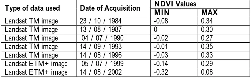
NDVI is determined using ER Mapper 7.0 for all seven (7) satellite images in the region of Neas Makris. The minimum and maximum NDVI values of each image are retrieved from the apt histograms and represented in Table 3.

Table 3: Min and Max values for NDVI

Type of data used Date of Acquisition NDVI Values

MIN MAX

Landsat TM image 23 / 10 / 1984 -0.08 0.34

Landsat TM image 13 / 08 / 1987 0 0.30

Landsat TM image 04 / 07 / 1990 -0.02 0.27

Landsat TM image 14 / 09 / 1993 -0.01 0.35

Landsat TM image 14 / 08 / 1996 -0.03 0.33

Landsat ETM+ image 05 / 07 / 1999 -0.14 0.29

(11)

The minimum and maximum values for NDVI are correspondingly applied to each image with the emphasis on the vegetation range of [±0.08;±0.35] as per results presented in Table 3. Each image with its own min and max values of NDVI is classified into three (3) equal classes, which are applied to the apt histograms using ER Mapper 7.0 software. Categorization of remotely sensed data requires the each pixel assignment of the image to the class. The electromagnetic spectral information in the original and altered bands is employed to portray each class pattern and to differentiate between classes (Ayanz and Biging, 1997). All classified Landsat TM and ETM+ images are saved as 8-bit binary images. Fragstat 3.3 program is used to examine species and ecosystems stages biodiversity concept (Figure 1 and Table 1). The inputs are seven (7) classified data into three (3) classes with 30m cell size of 8-bit binary images, 316 number of rows and 282 number of columns. RS metrics computations, results and discussions are performed according to biodiversity perception as per species and ecosystems stages

3. Results and Discussion

3.1 Results

In the paper of Petrosyan and Karathanassi (2011), an extensive investigation of the literature has been performed to gather, categorize and evaluate all landscape metrics based on RS data appearing in the literature through their use. Metrics classification results in six (6) out of seven (7) groups in the combination of the 2nd

(12)

Table 4: RS Metrics Categorization as per Authors Papers

No Groups Categories Authors

Papers

Tables RS Metrics Figures

1. Area /

Density / Edge

10 22 5 Number of Patches (NP) 4

Patch Density (PD) 5

Largest Patch Index(LPI) 6

Mean Value Patch Area (AREA_MN)

7

2. Shape 13 17 6 Mean Value of Shape Index

(SHAPE_MN)

8

Mean Value Contiguity Index (CONTIG_MN)

9

3. Core 7 Mean Value Core Area

(CORE_MN)

10

4. Isolation

Proximity

2 15 8 Mean Value Proximity

Index (PROX_MN)

11

5. Connectivity 2 5 9 Connectance Index

(CONNECT)

12

6. Contagion

Interspersion

8 12 10 Interspersion Juxtaposition

Index (IJI)

13

7. Diversity 9 20 11 Shannon’s Diversity Index

(SHDI)

14

Shannon’s Evennes Index (SHEI)

15

(13)

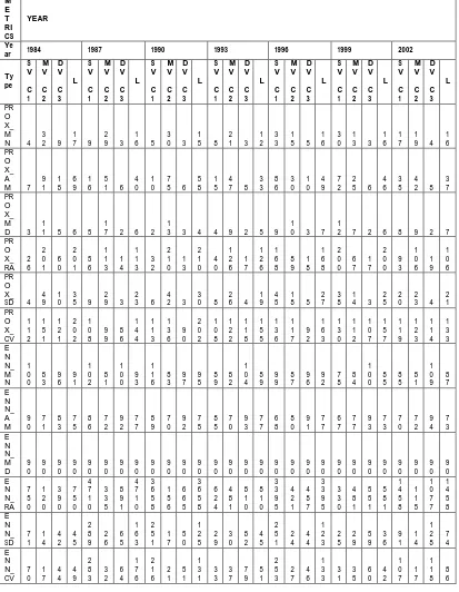
Table 5: Area / Edge / Density M ET RI CS YEAR Yea

r 1984 1987 1990 1993 1996 1999 2002

Ty pe S V C 1 M V C 2 D V C 3 L S V C 1 M V C 2 D V C 3 L S V C 1 M V C 2 D V C 3 L S V C 1 M V C 2 D V C 3 L S V C 1 M V C 2 D V C 3 L S V C 1 M V C 2 D V C 3 L S V C 1 M V C 2 D V C 3 L CA 2 6 8 2. 2 C 6 4 3 8 C 5 7 8 2. 2 C 3 2 8 8 C 3 4 3 2. 4 C 4 4 5 8 C 1 . 1 C 1. 9 C 2 5 1 8 C 1 . 1 C 1. 6 C 4 1 2 8 C 1 . 5 C 1. 5 C 1 9 8 7 . 9 C C

1. 9 C 2 2 5 7 . 9 C CP LA ND 3

2

8 8 - 7 2

8 4 - 4 2 9 6 -

1 4

2 3 3

1 5

1 9 5 -

1 8

1 8 2 -

1 3

2 3 3 - NP 2 1 7 3 6 2 2 6 9 8 5 3 2 6 2 3 6 6 2 4 7 8 8 0 2 3 4 4 1 9 3 7 7 C

4 8 9 4 5 7 2 2 1 C

1 8 1 4 0 2 2 1 5 8 0 3 2 9 2 5 0 6 1 5 9 9 6 2 3 4 8 5 2 6 1 6 1 C PD 3 5 3

1

1 3 5 3 1

1 3 5 5 1

3 6 6 3 1

5 2 5 3 1

0 4 6 2 1

2 4 7 2 1 3 LPI 0 . 1 0. 5 0. 1 0 . 5 0 . 1 0. 2 0. 1 0 . 2 0 . 1 0. 5 0. 1 0 . 5 0 . 2 0. 3 0. 1 0 . 3 0 . 4 0. 2 0. 1 0 . 4 0 . 5 0. 2 0. 1 0 . 5 0 . 2 0. 2 0. 1 0 . 2 TE 5 0 C 2 0 8 C 1 8 8 C 2 2 3 C 1 3 8 C 1 7 1 C 1 0 5 C 2 0 7 C 9 6 C 1 6 5 C 1 0 5 C 1 8 3 C 1 6 7 C 1 8 6 C 8 7 C 2 2 0 C 2 1 2 C 1 9 7 C 1 0 8 C 2 5 8 C 1 8 8 C 1 9 8 C 2 6 C 2 0 6 C 1 7 9 C 1 9 4 C 1 9 C 1 9 6 C ED 6

2 6 2 3 2 8 1 7 2 1 1 3 2 6 1 2 2 1 1 3 2 3 2 1 2 3 1 1 2 7 2 6 2 5 1 3 3 2 2 4 2 5 3

2 6

2 2

2 4 2

2 5 LSI 2 9 7 0 4 2 7

4 0

6 8

3 2 7

3 1

6 7

3 8 6

5 5

6 0

2 8 7

5 3

6 2

3 5 8

5 3

6 1

2 5 7

4 8

6 3

2 6 6 AR

EA _M

N 1 6 2 4 2 6 1 4 1 6 1 3 2 4 1 3 7 4 2 4 5 3 1 3 3 4 1 3 AR

EA _A M 2

1 7 5

1 3 4

1

1 2 9 3 1 4 2

1

1 5 9 3 7 1 6 8 4

1 0

1

3 6 3 9 6 8 3 7 AR

EA _M

D 1 3 1 2 1 5 1 2 1 3 1 1 1 2 1 1 3 2 1 2 3 2 1 2 2 2 1 2 AR

EA _R A 5

3 7 1 1 3 7 1 1 1 9 6

1 9 6

3 8 6

3 8

1 5

2 2 8

2 2

3 2

1 6 8

3 2

3 6

1 8 6

3 6

1 7

2 0 7

2 0 AR

EA _S

D 1 8 2 6 2 5 1 4 1 7 1 5 2 4 1 3 8 4 2 5 6 3 1 4 3 4 2 3 AR EA _C V 9 4 1 3 2 1 0 4 1 6 1 9 7 8 8 8 7 1 2 0 1 0 1 1 1 9 9 8 1 6 0 1 1 0 1 0 9 1 2 7 1 2 6 1 2 0 1 0 1 1 0 2 1 2 9 1 2 5 1 0 5 1 0 4 1 3 3 1 0 8 1 1 2 1 1 2 1 1 7 GY RA TE _M N 1 0 1 4 4 4 1 8 9 2 7 4 1 7 2 4 1 6 1 1 0 2 5 5 1 1 5 3 6 4 9 8 2 0 9 1 7 6 2 5 7 9 3 1 9 1 4 9 8 2 9 0 1 5 9 3 0 0 3 2 8 2 1 4 1 0 3 2 2 9 2 0 8 2 3 5 1 1 6 2 0 7 GY RA TE _A M 1 9 0 C

3 8 8 9 0 5 3 3 5 7 1 4 1 9 4 5 9 0 2 3 3 7 8 8 1 9 3 6 4 3 3 9 0 5 1 8 2 4 6 4 5 2 C

5 5 9 3 2 6 7 7 2 7 5 2 4 4 9 2 1 7 5 7 6 4 3 7 4 8 2 2 6 2 4 5 1 GY RA TE _M D 6 7 2 5 5 1 1 2 1 3 5 1 0 9 3 4 5 9 0 1 3 5 6 7 2 7 0 6 7 9 7 1 0 5 1 5 9 4 5 1 0 5 2 2 5 2 0 2 9 0 1 8 0 2 1 3 1 3 5 6 7 1 3 5 1 2 7 1 5 7 6 7 1 1 2 GY RA TE _R A 4 3 5 2. 4 C 9 0 2 2 . 4 C 9 5 2 1. 6 C 4 5 7 1 . 6 C 5 2 5 2 C 4 5 7 2 C 1 . 2 C 1. 3 C 6 7 7 1 . 3 C 2 . 3 C 1. 4 C 6 6 0 2 . 3 C 1 8 5 7 1. 5 C 5 4 2 1 . 9 C 1 . 3 C 1. 3 C 6 1 0 1 . 4 C GY RA TE _S D 9 5 5 3 2 1 9 4 3 9 6 1 7 0 3 5 9 9 6 2 9 0 1 1 8 3 6 9 9 7 2 7 9 1 9 7 2 5 1 1 2 1 2 1 7 5 8 8 2 7 8 1 6 3 3 7 2 3 5 0 2 3 0 1 0 9 2 7 0 2 1 9 2 3 1 1 3 1 2 1 8 GY RA TE _C V 9 4 1 2 0 1 0 3 1 4 5 9 9 8 6 8 8 1 1 3 1 0 3 1 0 1 9 9 1 3 4 1 1 2 9 8 1 3 0 1 1 4 1 1 8 9 6 1 0 3 1 2 4 1 0 7 1 0 7 1 0 5 1 1 8 1 0 5 9 8 1 1 3 1 0 6 NL SI 0 . 5 0. 4 0. 5 -

0 . 5 0. 4 0. 5 -

0 . 5 0. 5 0. 5 -

0 . 4 0. 5 0. 5 -

0 . 4 0. 4 0. 5 -

(14)

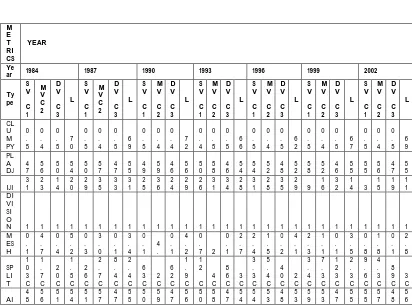
ME TR ICS

YEAR Yea

r 1984 1987 1990 1993 1996 1999 2002

Ty pe S V C 1 M V C 2 D V C 3 L S V C 1 M V C 2 D V C 3 L S V C 1 M V C 2 D V C 3 L S V C 1 M V C 2 D V C 3 L S V C 1 M V C 2 D V C 3 L S V C 1 M V C 2 D V C 3 L S V C 1 M V C 2 D V C 3 L SH AP E_ MN 1 . 8 3. 2 2 . 2 2 . 5 2 . 2 3 . 2 1 . 8 2 . 5 1 . 8 2 . 9 1 . 7 2 . 2 2 . 2 2. 5 1 . 6 2 . 2 3 . 3 2 . 8 2 . 1 2 . 7 2 . 8 2. 4 1 . 8 2 . 4 2 . 3 2. 5 1 . 9 2 . 3 SH AP E_ AM 2 . 4 5. 2 3 . 3 4 . 6 3 . 1 4 . 4 2 . 4 3 . 9 2 . 6 4 . 4 2 . 4 3 . 9 3 . 3 3. 7 2 . 6 3 . 5 5 . 6 4 . 0 3 . 1 4 . 5 4 . 2 3. 5 2 . 5 3 . 8 3 . 4 3. 6 2 . 8 3 . 4 SH AP E_ MD 1 . 7 2. 9 2 . 0 2 . 1 1 . 9 3 . 1 1 . 9 2 . 1 1 . 7 2 . 8 1 . 6 1 . 9 1 . 9 2. 3 1 . 4 1 . 9 2 . 7 2 . 5 1 . 9 2 . 5 2 . 5 2. 0 1 . 7 2 . 1 2 . 0 2. 2 1 . 7 2 . 0 SH AP E_ RA 2 . 8 6. 4 4 . 5 6 . 4 4 . 7 6 . 1 3 . 0 6 . 1 3 . 3 6 . 1 3 . 0 6 . 1 5 . 3 5. 2 3 . 7 5 . 3 7 . 0 5 . 8 3 . 8 7 . 0 5 . 5 5. 7 3 . 2 5 . 7 5 . 2 5. 2 3 . 6 5 . 2 SH AP E_S D 0 . 7 1. 7 1 . 1 1 . 5 1 . 0 1 . 5 0 . 7 1 . 3 0 . 8 1 . 5 0 . 7 1 . 2 1 . 1 1. 2 0 . 8 1 . 1 2 . 0 1 . 3 1 . 0 1 . 5 1 . 3 1. 2 0 . 7 1 . 2 1 . 1 1. 1 0 . 8 1 . 1 SH AP E_ CV 4 0 5 5 5 0 5 9 4 5 4 8 3 9 5 3 4 3 5 0 4 2 5 5 5 0 4 8 4 8 5 2 6 1 4 8 4 9 5 6 4 6 4 9 4 0 5 0 4 6 4 4 4 3 4 6 FR AC _M N 1 . 1 1. 2 1 . 1 1 . 2 1 . 1 1 . 2 1 . 1 1 . 2 1 . 1 1 . 2 1 . 1 1 . 1 1 . 1 1. 2 1 . 1 1 . 1 1 . 2 1 . 2 1 . 1 1 . 2 1 . 2 1. 2 1 . 1 1 . 2 1 . 2 1. 2 1 . 1 1 . 2 FR AC _A M 1 . 2 1. 3 1 . 2 1 . 3 1 . 2 1 . 3 1 . 2 1 . 2 1 . 2 1 . 2 1 . 2 1 . 2 1 . 2 1. 2 1 . 2 1 . 2 1 . 3 1 . 2 1 . 2 1 . 3 1 . 2 1. 2 1 . 2 1 . 2 1 . 2 1. 2 1 . 2 1 . 2 FR AC _M D 1 . 1 1. 2 1 . 2 1 . 2 1 . 1 1 . 2 1 . 1 1 . 2 1 . 1 1 . 2 1 . 1 1 . 1 1 . 1 1. 2 1 . 1 1 . 1 1 . 2 1 . 2 1 . 1 1 . 2 1 . 2 1. 2 1 . 1 1 . 2 1 . 2 1. 2 1 . 1 1 . 2 FR AC _R A 0 . 3 0. 3 0 . 3 0 . 3 0 . 3 0 . 3 0 . 3 0 . 3 0 . 3 0 . 3 0 . 3 0 . 3 0 . 3 0. 3 0 . 2 0 . 3 0 . 3 0 . 3 0 . 3 0 . 3 0 . 3 0. 3 0 . 2 0 . 3 0 . 3 0. 3 0 . 2 0 . 3 FR AC _S D 0 . 1 0. 1 0 . 1 0 . 1 0 . 1 0 . 1 0 . 1 0 . 1 0 . 1 0 . 1 0 . 1 0 . 1 0 . 1 0. 1 0 . 1 0 . 1 0 . 1 0 . 1 0 . 1 0 . 1 0 . 1 0. 1 0 . 1 0 . 1 0 . 1 0. 1 0 . 1 0 . 1 FR AC _C V 6 . 0 7. 4 7 . 1 7 . 6 6 . 3 7 . 0 5 . 9 7 . 1 5 . 9 7 . 4 6 . 2 7 . 3 6 . 8 6. 8 6 . 2 7 . 0 7 . 8 6 . 9 6 . 9 7 . 4 6 . 1 6. 6 5 . 4 6 . 6 6 . 1 6. 0 5 . 6 6 . 1 PA RA _M N 7 7 9 6 9 5 7 4 2 7 3 4 7 2 1 6 5 9 7 7 0 7 1 2 7 5 2 6 8 3 7 8 9 7 4 0 7 4 1 6 8 7 7 9 0 7 3 1 6 9 9 7 1 0 7 5 9 7 2 4 6 6 2 7 0 9 7 6 2 7 0 6 6 8 9 6 8 6 7 5 6 7 0 1 PA RA _A M 7 0 9 5 8 9 6 6 4 6 1 5 6 6 2 5 7 4 7 1 2 6 0 5 6 7 8 5 5 2 7 1 8 5 9 0 6 6 9 5 6 5 7 1 7 6 1 3 6 1 6 6 3 8 6 9 8 6 3 7 5 5 8 6 3 9 7 1 5 6 0 6 6 0 4 5 8 3 7 1 0 5 9 9 PA RA _M D 7 4 1 6 8 5 7 1 1 7 0 4 7 1 1 6 7 7 7 2 2 7 0 4 7 4 1 6 8 2 7 4 1 7 1 8 7 1 4 6 9 1 7 7 8 7 1 1 6 8 8 6 9 1 7 2 2 6 9 4 6 8 4 6 9 8 7 4 1 6 9 8 6 9 8 6 9 8 7 4 1 7 0 4 PA RA _R A 8 5 7 9 3 9 4 8 1 9 3 9 5 6 1 9 7 5 6 5 6 9 7 5 9 3 3 9 8 5 6 5 6 9 8 5 9 7 0 9 6 1 4 1 7 9 7 0 9 0 8 9 4 4 6 5 9 9 4 4 9 7 0 9 3 3 2 1 3 9 7 0 9 6 6 9 3 9 2 1 4 9 6 6 PA RA _S D 1 1 0 1 1 7 1 0 2 1 2 3 9 8 1 4 2 1 0 3 1 3 5 1 1 4 1 6 5 1 1 4 1 4 9 1 2 2 1 6 3 8 6 1 4 4 1 2 6 1 1 3 9 0 1 2 1 1 2 8 1 2 2 7 1 1 2 8 1 2 9 1 2 4 6 6 1 2 8 PA RA _C V 1 4 1 7 1 4 1 7 1 4 2 1 1 3 1 9 1 5 2 4 1 4 2 0 1 7 2 4 1 1 2 0 1 8 1 6 1 2 1 7 1 9 1 7 9

1 8

1 9

1 8 9

1 8 CIR CL E_ MN 0 . 8 0. 9 0 . 8 0 . 0 0 . 9 0 . 9 0 . 8 0 . 0 0 . 8 0 . 9 0 . 8 0 . 0 0 . 8 0. 9 0 . 8 0 . 0 0 . 9 0 . 9 0 . 8 0 . 0 0 . 9 0. 9 0 . 8 0 . 0 0 . 9 0. 9 0 . 8 0 . 0

(15)

ME TR ICS

YEAR Yea

r 1984 1987 1990 1993 1996 1999 2002

Ty pe S V C 1 M V C 2 D V C 3 L S V C 1 M V C 2 D V C 3 L S V C 1 M V C 2 D V C 3 L S V C 1 M V C 2 D V C 3 L S V C 1 M V C 2 D V C 3 L S V C 1 M V C 2 D V C 3 L S V C 1 M V C 2 D V C 3 L CL E_ AM . 9

0 . 0 . 0 . 9 . 0 . 9 . 0 . 9 . 0 . 9 . 0 . 9

0 . 9 . 0 . 0 . 0 . 9 . 0 . 0

0 . 9

. 0

(16)

Table 7: Core Area M ET RI CS YEAR Ye

ar 1984 1987 1990 1993 1996 1999 2002

Ty pe S V C 1 M V C 2 D V C 3 L S V C 1 M V C 2 D V C 3 L S V C 1 M V C 2 D V C 3 L S V C 1 M V C 2 D V C 3 L S V C 1 M V C 2 D V C 3 L S V C 1 M V C 2 D V C 3 L S V C 1 M V C 2 D V C 3 L TC A 2 6 8 2 . 2 C 6 4 3 3 . 2 C 5 7 8 2 . 3 C 3 2 8 3 . 2 C 3 4 3 2 . 5 C 4 4 5 3 . 2 C C

1 . 8 C 2 5 1 3 . 2 C 1 . 2 C 1 . 5 C 4 1 2 3 . 2 C 1 . 5 C 1 . 5 C 1 9 8 3 . 1 C C

1 . 9 C 2 2 5 3 C CP LA ND 3

2 8

8 . 0 - 7

2 8

4 . 1 - 4

2 9

5 . 5 -

1 4 2 3 3 . 1 -

1 5 1 9 5 . 1 -

1 8 1 8 2 . 5 -

1 3 2 3 2 . 8 -

ND CA 2 1 7 3 6 2 2 6 9 8 5 3 2 6 2 3 6 6 2 4 7 8 8 0 2 3 4 4 1 9 3 7 7 C

4 8 9 4 5 7 2 2 1 C

1 8 1 4 0 2 2 1 5 8 0 3 2 9 2 5 0 6 1 5 9 9 6 2 3 4 8 5 2 6 1 6 1 C

DC AD 2 . 7 4 . 5 3 . 4 1 1 3 . 3 4 . 6 3 . 1 1 1 2 . 9 5 . 2 4 . 7 1 3 6 . 1 5 . 7 2 . 8 1 5 2 . 3 5 . 0 2 . 7 1 0 3 . 7 6 . 4 2 . 0 1 2 4 . 4 6 . 6 2 . 0 1 3 CO RE _M N 1 . 2 6 . 2 2 . 4 3 . 7 2 . 2 6 . 1 1 . 3 3 . 6 1 . 5 5 . 6 1 . 2 3 . 0 2 . 2 3 . 9 1 . 1 2 . 7 6 . 6 3 . 8 1 . 9 3 . 9 5 . 0 2 . 9 1 . 2 3 . 2 3 . 0 3 . 5 1 . 4 3 . 0 CO RE _A

M 2

1 7 5 . 0 1 3 4

1 1

2 . 3 9 3

1 4 2 . 3 1 1 5 9

3 . 0 7

1 6 8

3 . 9 1 0 1 3 6

2 .

6 9 6 8 3 . 1 7 CO RE _M D 0 . 8 3 . 2 1 . 4 1 . 6 1 . 3 4 . 6 1 . 1 1 . 6 0 . 8 3 . 4 0 . 8 1 . 2 1 . 3 2 . 2 0 . 5 1 . 4 2 . 7 2 . 4 1 . 1 2 . 2 2 . 7 1 . 8 0 . 8 1 . 6 1 . 6 1 . 9 0 . 8 1 . 6 CO RE _R

A 5

3 7 1 1 3 7 1 1 1 9 6

1 9 6

3 8 6

3 8

1 5

2 2 8

2 2

3 2

1 6 8

3 2

3 6

1 8 6

3 6

1 7

2 0 7

2 0 CO RE _S D 1 . 2 8 . 2 2 . 5 5 . 9 2 . 1 5 . 4 1 . 2 4 . 3 1 . 5 6 . 7 1 . 2 4 . 9 2 . 4 4 . 3 1 . 4 3 . 4 7 . 9 3 . 8 2 5

6 . 2 3

1 . 3 4 . 3 3 . 2 3 . 9 1 . 6 3 . 5 CO RE _C V 9 4 1 3 2 1 0 4 1 6 1 9 7 8 8 8 7 1 2 0 1 0 1 1 1 9 9 8 1 6 0 1 1 0 1 0 9 1 2 7 1 2 6 1 2 0 1 0 1 1 0 2 1 2 9 1 2 5 1 0 5 1 0 4 1 3 3 1 0 8 1 1 2 1 1 2 1 1 7 DC OR E_ M N 1 . 2 6 . 2 2 . 4 3 . 7 2 . 2 6 . 1 1 . 3 3 . 6 1 . 5 5 . 6 1 . 2 3 . 0 2 . 2 3 . 9 1 . 1 2 . 7 6 . 6 3 . 8 1 . 9 3 . 9 5

2 . 9 1 . 2 3 . 2 3

3 . 5

1 . 4 3 DC

OR E_ AM 2

1 7 5 . 0 1 3 4

1 1

2 . 3 9 3

1 4 2 . 3 1 1 5 9

3 . 0 7

1 6 8

3 . 9 1 0 1 3 6

2 .

6 9 6 8 3 . 1 7 DC OR E_ M D 0 . 8 3 . 2 1 . 4 2

1 . 3 4 . 6 1 . 1 2

0 . 8 3 . 4 0 . 8 1

1 . 3 2 . 2 0 . 5 1

2 . 7 2 . 4 1 . 1 2

2 . 7 1 . 8 0 . 8 2

1 . 6 1 . 9 0 . 8 2 DC

OR E_ RA 5

3 7 1 1 3 7 1 1 1 9 5 . 6 1 9 6

3 8 5 . 6 3 8 1 5 2 2 8 . 1 2 2 3 2 1 6 8

3 2 3 6 1 8 6 . 5 3 6 1 7 2 0 7 . 3 2 0 DC OR E_ SD 1 . 2 8 . 2 2 . 5 5 . 9 2 . 1 5 . 4 1 . 2 4 . 3 1 . 5 6 . 7 1 . 2 4 . 9 2 . 4 4 . 3 1 . 4 3 . 4 7 . 9 3 . 8 2 . 0 5 . 0 6 . 2 3 . 0 1 . 3 4 . 3 3 . 2 3 . 9 1 . 6 3 . 5

(17)

M ET RI CS

YEAR

Ye

ar 1984 1987 1990 1993 1996 1999 2002

Ty pe

S V

C 1

M V

C 2

D V

C 3

L S V

C 1

M V

C 2

D V

C 3

L S V

C 1

M V

C 2

D V

C 3

L S V

C 1

M V

C 2

D V

C 3

L S V

C 1

M V

C 2

D V

C 3

L S V

C 1

M V

C 2

D V

C 3

L S V

C 1

M V

C 2

D V

C 3

L

OR E_ CV

4 3 2

0 4

6 1

7 8 7 2 0

0 1

1 9

8 6 0

1 0

0 9

2 7

2 6

2 0

0 1

0 2

2 9

2 5

0 5

0 4

3 3

0 8

1 2

1 7

CA I_ M N

1 0 0

1 0 0 CA

I_A M

1 0 0

1 0 0 CA

I_ M D

1 0 0

1 0 0 CA

I_R

A 0 0 0 0 0 0 0 0 0 0 0 0 0 0 0 0 0 0 0 0 0 0 0 0 0 0 0 0 CA

I_S

D 0 0 0 0 0 0 0 0 0 0 0 0 0 0 0 0 0 0 0 0 0 0 0 0 0 0 0 0 CA

I_C

(18)

Table 8: Isolation Proximity M E T RI CS YEAR Ye

ar 1984 1987 1990 1993 1996 1999 2002

Ty pe S V C 1 M V C 2 D V C 3 L S V C 1 M V C 2 D V C 3 L S V C 1 M V C 2 D V C 3 L S V C 1 M V C 2 D V C 3 L S V C 1 M V C 2 D V C 3 L S V C 1 M V C 2 D V C 3 L S V C 1 M V C 2 D V C 3 L PR O X_ M N 4

3 2 9

1 7 9

2 9 3

1 6 5

3 0 3

1 5 8

2 1 3

1 2

3 3

1 5 5

1 6

3 0

1 3 3

1 6

1 7

1 9 4

1 6 PR O X_ A M 7

9 1 1 8 6 9 1 6 5 1 6

4 0

1 0

7 5 6

5 8

1 5

4 7 8

3 3 8 6 3 0 1 0 4 9 7 2 2 5 6

4 6

3 5

4 2 8

3 7 PR O X_ M D 3

1

1 5 6 5 1

7 2 6 2 1

3 3 4 4 9 2 5 9 1 0 3 7

1

2 7 2 6 8 9 2 7 PR O X_ RA 2 6 2 0 1 6 0 2 0 1 5 6 1 1 3 1 4 1 1 3 3 2 2 1 0 1 3 2 1 0 4 0 1 2 6 1 7 1 2 6 1 6 8 8 9 1 8 1 6 8 2 0 0 6 7 1 7 2 0 0 9 3 1 0 6 1 9 1 0 6 PR O X_ SD 4

4 9

1 0

3 5 9

2 9 3

2 3 6

4 2 3

3 0 8

2 6 4

1 9

4 5

1 8 5

2 7

3 8

1 4 3

2 5

2 0

2 3 4

(19)

Table 9: Connectivity ME TR ICS YEAR Yea

r 1984 1987 1990 1993 1996 1999 2002

Ty pe S V C 1 M V C 2 D V C 3 L S V C 1 M V C 2 D V C 3 L S V C 1 M V C 2 D V C 3 L S V C 1 M V C 2 D V C 3 L S V C 1 M V C 2 D V C 3 L S V C 1 M V C 2 D V C 3 L S V C 1 M V C 2 D V C 3 L CO NN EC T 0 . 8 0 . 6 0 . 7 0 . 7 0 . 8 0 . 6 0 . 7 0 . 7 0 . 8 0 . 5 0 . 5 0 . 6 0 . 4 0 . 5 0 . 8 0 . 5 1 . 1 0 . 5 0 . 8 0 . 7 0 . 8 0 . 4 1 . 0 0 . 5 0 . 6 0 . 4 1 . 1 0 . 5 CO HE SIO N 7 9 9 2 8 6 9 1 8 5 9 1 7 9 8 9 8 1 9 1 7 9 8 9 8 6 8 9 8 1 8 8 9 2 8 9 8 4 9 0 9 1 8 7 8 0 8 9 8 7 8 8 8 2 8 8

Table 10: Contagion Interspersion

M E T RI CS YEAR Ye

ar 1984 1987 1990 1993 1996 1999 2002

Ty pe S V C 1 M V C 2 D V C 3 L S V C 1 M V C 2 D V C 3 L S V C 1 M V C 2 D V C 3 L S V C 1 M V C 2 D V C 3 L S V C 1 M V C 2 D V C 3 L S V C 1 M V C 2 D V C 3 L S V C 1 M V C 2 D V C 3 L CL U M PY 0 . 5 0 . 4 0 . 5 7 0 0 . 5 0 . 4 0 . 5 6 9 0 . 5 0 . 4 0 . 4 7 2 0 . 4 0 . 5 0 . 5 6 6 0 . 5 0 . 4 0 . 5 6 2 0 . 5 0 . 4 0 . 5 6 7 0 . 5 0 . 4 0 . 5 6 9 PL A DJ 4 7 5 6 5 0 5 4 5 0 5 7 4 7 5 5 4 9 5 9 4 6 5 6 5 0 5 8 4 6 5 4 5 4 5 2 4 8 5 2 5 8 5 2 4 6 5 5 5 5 5 6 4 7 5 5 IJI 3 1 2 3 1 4 2 0 2 9 3 5 3 3 3 1 2 5 3 6 2 4 2 9 2 6 3 1 3 4 2 8 3 1 2 8 3 5 2 9 9

1 6

3 2

1 4 3

1 5 1 9 1 1 DI VI SI O

N 1 1 1 1 1 1 1 1 1 1 1 1 1 1 1 1 1 1 1 1 1 1 1 1 1 1 1 1 M ES H 0 . 1 4 . 7 0 . 4 5 . 2 0 . 3 3 . 0 0 . 1 3 . 4 0 . 1 4 . 0 . 1 4 . 2 0 . 7 2

(20)

Table 11: Diversity Where C=1000.

METRICS YEAR

Year 1984 1987 1990 1993 1996 1999 2002

Type L L L L L L L

PR 8 8 8 8 8 8 8

PRD 0.1 0.1 0.1 0.1 0.1 0.1 0.1

RPR 267 267 267 267 267 267 267

SHDI 0.8 0.8 0.7 0.9 1.0 0.9 0.9

SIDI 0.4 0.4 0.4 0.5 0.6 0.6 0.5

MSIDI 0.6 0.6 0.5 0.8 0.9 0.8 0.8

SHEI 0.4 0.4 0.4 0.4 0.5 0.4 0.4

SIEI 0.5 0.5 0.5 0.6 0.7 0.6 0.6

MSIEI 0.3 0.3 0.3 0.4 0.4 0.4 0.4

classes are as:

RS metrics are calculated to observe the state of the land. NDVI is computed to monitor the condition of vegetation. Categorization of three (3) equal classes is performed to the distribution with the defined min and max values of NDVI in Table 3. The

0 4 8 12 16

1984 1987 1990 1993 1996 1999 2002

Figure 5: PD

0 0.2 0.4 0.6

1984198719901993199619992002

Figure 6: LPI

Speci es Ecosy stems

0 500 1000 1500

1984 1987 1990 1993 1996 1999 2002

(21)

0 2 4 6 8

1984 1987 1990 1993 1996 1999 2002

Figure10: CORE_MN

0 10 20 30 40

1984198719901993199619992002

Figure 11: PROX_MN

0 0.3 0.6 0.9 1.2

1984198719901993199619992002

Figure 12: CONNECT

0 10 20 30 40

1984198719901993199619992002

Figure 13: IJI

0.5 0.7 0.9 1.1

19841987 19901993 19961999 2002

Figure 14: SHDI

0 0.2 0.4 0.6

1984198719901993199619992002

Figure 13: SHEI

Figure 15: SHEI

Figure 5: AREA_MN

0 2 4 6 8

1984198719901993199619992002 Figure

7:AREA_

0.25 0.3 0.35 0.4

1984 1987 1990 1993 1996 1999 2002

Figure 9: CONTIG_MN

1 2 3 4

1984 19871990 19931996 19992002

(22)

3.2 Biodiversity Indicators at Species (Classes) Stage

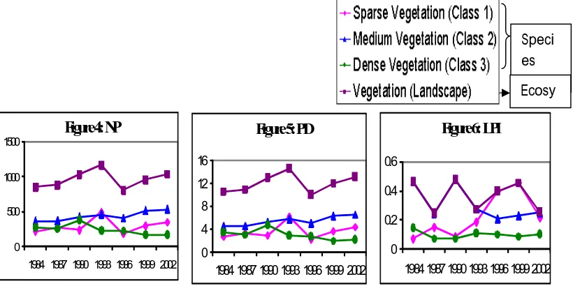
The biodiversity metrics at species stage assess the summative properties of the patches and fit into a particular class or patch type (Giordano & Marini, 2008). The time series of classified satellite images are the sources for the landscape metrics computation at species stages using Fragstat software as a tool. Graphs of species biodiversity stage are depicted on Figures 4-13, issued as per Table 4, combined in Tables 5-10 & applied as:

 Pink = Sparse Vegetation (SV) = Class 1 (C1) = α

diversity;

 Blue = Medium Vegetation (MV) = Class 2 (C2) =

β diversity;

 Green = Dense Vegetation (DV) = Class 3 (C3) =

γ diversity.

3.2.1 Sparse Vegetation (Class 1 - α diversity)

Sparse vegetation (SV = C1 = α diversity) in this paper represents the minor class of landscape (Tables 5-10 and Figures 4-13). Furthermore, sparse vegetation

(class 1) corresponds to α diversity in species biodiversity stage. The study shows an

increase with some variations in the number of patches (NP) (Figure 4), the patch density (PD) (Figure 5), the largest patch index (LPI) (Figure 6) and mean value of patch area (AREA_MN) (Figure 7) during the period from 1984 to 2002. In addition, the highest values of mean shape index (SHAPE_MN) (Figure 8), mean contiguity index (CONTIG_MN) (Figure 9), mean core area (CORE_MN) (Figure 10), mean proximity index (PROX_MN) (Figure 11) and connectance index (CONNECT) (Figure 12) are in the year of 1996. There is also a decrease in the interspersion juxtaposition index (IJI) (Figure 13) mainly between 1996 and 2002.

3.2.2 Medium Vegetation (Class 2 - β diversity)

Medium vegetation (MV = C2 = β diversity) in the current study is characterized as the major class of landscape (Tables 5-10 and Figures 4-13). Moreover, medium vegetation (Class 2) goes with β diversity in species biodiversity

(23)

Furthermore, there is a decrease in the values of the largest patch index (LPI) (Figure 6), mean value of patch area (AREA_MN) (Figure 7), mean core area (CORE_MN) (Figure 10), mean proximity index (PROX_MN) (Figure 11) and the interspersion juxtaposition index (IJI) (Figure 13) from the time period from 1984 to 2002. Moreover, there is a somehow stability in the in the values of mean shape index (SHAPE_MN) (Figure 8), mean contiguity index (CONTIG_MN) (Figure 9) and connectance index (CONNECT) (Figure 12) during the period from 1984 to 2002.

3.2.3 Dense Vegetation (Class 3 - γ diversity)

Dense vegetation (DV = C3 = γ diversity) in the present study is illustrated as the medium to minor class of landscape (Tables 5-10 and Figures 4-13). Additionally,

dense vegetation (class 3) matches with γ diversity in species biodiversity stage. The study shows stabilization with small variation in terms of the number of patches (NP) (Figure 4), the patch density (PD) (Figure 5), the largest patch index (LPI) (Figure 6), mean value of patch area (AREA_MN) (Figure 7), mean shape index (SHAPE_MN) (Figure 8), mean contiguity index (CONTIG_MN) (Figure 9), mean core area (CORE_MN) (Figure 10) and mean proximity index (PROX_MN) (Figure 11) from the time period from 1984 to 2002. Furthermore, there are augments in the values of connectance index (CONNECT) (Figure 12) and variations in the values of the interspersion juxtaposition index (IJI) (Figure 13) in the years of 1990 and 2002.

3.3 Biodiversity Indicators at Ecosystems (Landscape) Stage

(24)

There is kind of stability in the mean value of contiguity index (CONTIG_MN) (Figure 9). The values of the connectance index (CONNECT) (Figure 12) and interspersion juxtaposition index (IJI) (Figure 13) are increased for the years of 1984 – 1987, stabilized for the years of 1987 – 1996 and decreased for the years of 1996-2002. There is a kind of stabilization for the time period of 1984 – 1990 and 1996 – 2002 and augment for the years of 1990 – 1996 for the Shannon Diversity (SHDI) (Figure 14) and evenness (SHEI) (Figure 15) indices. Shannon’s diversity index is a popular appraisal of diversity in ecology applied to landscapes as a measure of the equitability in NP as per proportional area distribution along with patch types. Shannon evenness index is accepted diversity appraisal employed in ecology signifying the evenness of the area distribution in company with the different patch types (McGarigal etc, 2002).

4. Conclusion

The investigations of species biodiversity stage explain that the landscape of the study area is dominated with the medium vegetation (MV = C2 = β diversity), followed by dense vegetation (DV = C3 = γ diversity) and sparse vegetation (SV = C1 = α diversity). During the study period of (1984 – 2002), medium and dense vegetation are decreased while sparse vegetation is increased. Therefore, an increase of urban areas expresses a change from the vegetated spots to the non-vegetated areas.

(25)

Reference

ANZECC, (2000). Core Environmental Indicators for Reporting on the State of the Environment. Canberra: Environment Australia.

Argialas, D. P. (2000). Φωτοερμηνεία-Τηλεσκόπηση. Έκδοση Εθνικού Μετσοβιού Πολυτεχνείου.

Ayanz, J. S. M., & Biging, S. (1997). Comparison of Single-Stage and Multi-Stage Classification Approaches for Cover Type Mapping with TM and SPOT Data. Remote Sensing of Environment 59, 92-104.

Ayanz, J. S. M. (1996). Synergy of optical and polarimetric microwave data for forest resource assessment. International Journal of Remote Sensing, 17 (18), 3647-3663.

ER MAPPER, (2005). ER Mapper Version 7. User Guide.

ERDAS, (2005). Erdas Imagine 9.0 Tour Guide. Leica Geosystems Geospatial Imaging, LLC. ERDAS, (1997). ERDAS Field Guide. 4th ed. ERDAS Inc., Atlanta, Georgia.

ESRI, (1997). Understanding GIS, The Arc/Info method, version 7.1 for Unix and Windows NT. John Viley & Sons Inc., New York.

ESRI, (1994). PC Arc / Info. Command References. Redlands, CA.

Fazey, I., Fischer, J., & Lindenmayer, D. B. (2005). What do conservation biologists publish? Biological Conservation, 124, 63–73.

Fischer, J., & Lindenmayer, D. B., (2007). Landscape modification and habitat fragmentation: a synthesis. Global Ecology and Biogeography, 16, 265–280.

Foley, J. A., DeFries, R., Asner, G. P., Barford, C., Bonan, G., Carpenter, S. R., Chapin, F. S., Coe, M. T., Daily, G. C., Gibbs, H. K., Helkowski, J. H., Holloway, T., Howard, E. A., Kucharik, C. J., Monfreda, C., Patz, J. A., Prentice, I. C., Ramankutty, N., & Snyder, P. K. (2005). Global consequences of land use. Science, 309, 570–574. Foody, G. M. (2003). Remote Sensing of tropical forest environments: towards the

monitoring of environmental resources for sustainable development. International Journal Remote Sensing, 24(20), 4035-4046.

Giordano, F., & Marini, A. (2008). A Landscape Approach for Detecting and Assessing Changes in an Area Prone to Desertification in Sardinia (Italy). International Journal of Navigation and Observation, 5pp.

Greco, M., Mirauda, D., Squicciarino, G., & Telesca, V. (2005). Desertification risk assessment in Southern Mediterranean areas. Advanced Geoscience, 2, 243-247. Hall, J. P. (2001). Criteria and indicators of sustainable forest management. Environmental

Monitoring and Assessment, 67, 109–119.

Jensen, J. R. (2000). Remote Sensing of the Environment. An Earth Resource Perspective. Prentice Hall. Upper Saddle River, New Jersey.

Kosioni-Koen, M., & Papastergiou-Mitsopoulou, E. (2004). General scheme for the urban-planning: The Municipality of Neas Makris. Prefectional Self-Administration of East Athens.

(26)

Lopez-Bermudez, F., & Garcia Gomez, J. (2003). Desertification in the arid and semiarid Mediterranean regions. NATO-CCMS and Science Committee Workshop on Desertification in the Mediterranean Region, A Food Security Issue, 2-5 December 2003, Valencia (Spain).

Mahiny, A. S., & Turner, B. J. (2005). Cumulative Effects Assessment as a Framework for Prioritizing Mitigation Measures in Remnants of Vegetation. Environmental Informatics Archives, 3, 418 - 426.

McDermid, G. J., Franklin, S. E., & LeDrew, E. F. (2005). Remote sensing for large-area habitat mapping. Progress in Physical Geography, 29, 449–474.

McGarigal, K., Cushman, S. A., Neel, M. C., & Ene, E. (2002). FRAGSTATS: Spatial Pattern Analysis Program for Categorical Maps. Computer software program produced by the authors at the University of Massachusetts, Amherst. [Online]

Available: www.umass.edu/landeco/research/fragstats/fragstats.html.

McGarigal, K., & Marks, B. (1995). FRAGSTATS: Spatial Pattern Analysis Program for Quantifying Landscape Structure. General Technical Report. PNW-GTR-351. U.S. Department of Agriculture, Forest Service, Pacific Northwest Research Station, Portland, OR. [Online]. Available:

http://www.umass.edu/landeco/research/fragstats/fragstats.html.

Melesse, A. M., Weng, Q. H., Thenkabail, P. S., & Senay, G. B. (2007). Remote sensing sensors and applications in environmental resources mapping and modeling. Sensors, 7, 3209–3241.

Nagler, P. L., Glenn, E. P., & Hinojosa-Huerta, O. (2009). Synthesis of ground and remote sensing data for monitoring ecosystem functions in the Colorado River Delta, Mexico. Remote Sensing of Environment.

Parodi, G. N. (2002). AVHRR hydrological analysis systems: User manual version 1.3. AHAS User Guide. Enschede, ITC.

Peter, M., Edwards, P. J., Jeanneret, P., Kampmann, D., Luscher, A., (2008). Changes over three decades in the floristic composition of fertile permanent grasslands in the Swiss Alps. Agriculture, Ecosystems and Environment, 125, 204–212.

Petrosyan, A. (2010). A Model for Incorporated Measurement of Sustainable Development Comprising Remote Sensing Data and Using the Concept of Biodiversity. Journal of Sustainable Development, 3 (2), 9-26.

Petrosyan, A. F., & Karathanassi, V. (2011). Review Article of Landscape Metrics based on Remote Sensing Data. Journal of Environmental Science and Engineering, 5 (11), 1542-1560.

Schreiber, K. V. (2006). An approach to monitoring and assessment of desertification using integrated geospatial technologies. In: Proceedings of the 17th_{Conference on}

Biometereology and Aerobiology, 24 May 2006, San Diego, CA.

Seaquist, J. W., Olsson, L., & Ardoc, J. (2003). A remote sensing-based primary production model for grassland biomes. Ecological Modelling, 169, 131–155.

Strand, H., Hoft, R., Strittholt, J., Horning, N., Miles, L., Fosnight, E., & Turner, W. (2007). Sourcebook on Remote Sensing and Biodiversity Indicators. CBD Technical Series No. 32: 205pp.

Symeonakis, E., & Drake, N. (2004). Monitoring desertification and land degradation over sub-Sahara Africa. International Journal of Remote Sensing, 25, 573 – 592.

(27)

Turner, R. K., Button, K., & Nijkamp, P. (1999). Ecosystems and Nature: Economics, Science and Policy. Edward Elgar, Cheltenham, UK and Northampton, MA, US. U.S. Environmental Protection Agency, (2002). A Framework for the Economic Assessment

of Ecological Assessment of Ecological Benefits. Ecological Benefit Assessment Workgroup, Social Sciences Discussion Group, Science Policy Council, U.S. Environmental Protection Agency.