www.ocean-sci.net/7/651/2011/ doi:10.5194/os-7-651-2011
© Author(s) 2011. CC Attribution 3.0 License.
Ocean Science
About uncertainties in practical salinity calculations
M. Le Menn
French Hydrographic and Oceanographic Service (SHOM), SHOM, CS 92803, 29228 Brest Cedex 2, France Received: 22 September 2009 – Published in Ocean Sci. Discuss.: 28 October 2009
Revised: 21 September 2011 – Accepted: 29 September 2011 – Published: 17 October 2011
Abstract. In the current state of the art, salinity is a quan-tity computed from conductivity ratio measurements, with temperature and pressure known at the time of the mea-surement, and using the Practical Salinity Scale algorithm of 1978 (PSS-78). This calculation gives practical salin-ity valuesS. The uncertainty expected in PSS-78 values is
±0.002, but no details have ever been given on the method used to work out this uncertainty, and the error sources to include in this calculation. Following a guide published by the Bureau International des Poids et Mesures (BIPM), using two independent methods, this paper assesses the uncertain-ties of salinity values obtained from a laboratory salinometer and Conductivity-Temperature-Depth (CTD) measurements after laboratory calibration of a conductivity cell. The re-sults show that the part due to the PSS-78 relations fits is sometimes as significant as the instrument’s. This is partic-ularly the case with CTD measurements where correlations between variables contribute mainly to decreasing the uncer-tainty of S, even when expanded uncertainties of conduc-tivity cell calibrations are for the most part in the order of 0.002 mS cm−1. The relations given here, and obtained with the normalized GUM method, allow a real analysis of the un-certainties’ sources and they can be used in a more general way, with instruments having different specifications.
1 Introduction
Salinity is one of the fundamental quantities for which mea-surement or computation is essential to determine the funda-mental properties of seawater. In the current state of the art, salinity is computed from conductivity ratio measurements, with temperature and pressure known at the time of mea-surement, and using the Practical Salinity Scale algorithm
Correspondence to: M. Le Menn
defined by Perkin and Lewis (1980). This algorithm gives practical salinities from the ratio of the electrical conductiv-ity of seawater at 15◦C related to that of a standard potassium chloride solution (KCl).
In practice, in laboratories, salinity is computed from a conductivity ratio measured with salinometers calibrated with IAPSO standard seawater bottles whose salinity and conductivity ratio at 15◦C or K15 are known. At sea, in-struments are equipped with conductivity cells calibrated and linearized in seawater baths whose temperature is controlled and measured with great accuracy and whose salinity is de-termined by salinometers.
The World Ocean Circulation Experiments (WOCE) pro-gramme suggested that temperature and conductivities could be measured respectively to 0.002◦C and 0.002 mS cm−1, re-sulting in a salinity measurement accuracy of±0.002 (Saun-ders et al., 1991), but no details were given on the method used to work out the uncertainty measurements and which error sources should be included in this calculation. Several Conductivity–Temperature-Depth (CTD) instruments manu-facturers propose equipment whose specifications are sup-posed to fill these criteria. However, which are really the un-certainties obtained on the measurements needed to establish or to check these criteria? A simple addition of uncertainties, as often seen in manuscripts, (cf. Uschida et al., 2008, for example) is incorrect because sensitivities and input quantity correlations must also be taken into account in the calcula-tions.
input variable. From the results, the software can produce a histogram of the output variable distribution and its varia-tion statistics (mean, standard deviavaria-tion, etc.). The GUM and Monte Carlo methods are two independent ways to calculate a measurement uncertainty.
The goal of this paper is to assess the uncertainties of practical salinity calculations using these two methods, when salinity is obtained from laboratory salinometer measure-ments or from CTD measuremeasure-ments after laboratory calibra-tion of conductivity cells.
2 Uncertainties on salinities calculated from salinome-ter measurements
Laboratory salinometers are calibrated with IAPSO standard seawater (SSW) bottles distributed by OSIL (www.OSIL.co. uk), which has the international exclusive rights to do so. The ratioK15 of the seawater bottle is determined by OSIL and written on each bottle. Then the conductivity cell of a salinometer at the temperaturet measures the conductivity Gst(t ), so that:
Gst(t )=K15C(35,15,0)kcellst (1) C(35, 15, 0) is the conductivity of standard seawater with a salinity of 35 at the temperature of 15◦C and the pressure of 0 dbar.kcellstis a value adjusted by the salinometer and which is inversely proportional to the cell constant at the time and the temperature of the measurement. For a seawater sample, the cell will measureG(t ), so that:
G(t )=RtrtC(35,15,0)kcell (2)
kcell being the value inversely proportional to the cell con-stant, at the time and the temperature of the measurement. Rt is the ratio displayed by the salinometer.Rt is equivalent
toK15for the seawater sample.rt is the temperature
correc-tion polynomial of the PSS-78, used to compensate for the temperature effect of the sample:
rt=c0+c1t+c2t2+c3t3+c4t4 (3) wherec0, c1,c2,c3andc4are constants given for the cal-culation of salinity (Perkin et al., 1980). See Appendix A to obtain the numerical values of the PSS-78 constants. If we callδkcellthe ratiokcellst/kcell,Rt is given by:
Rt= G(t ) Gst(t )
K15 rt
δkcell (4)
The relation (4) describes the conductivity ratio displayed by the salinometer and used to calculate the salinity. G(t )and Gst(t )are two quantities correlated by the temperature. The electrical conductivity signal is a function of salinity, tem-perature and pressure. However, under typical conditions it is admitted (cf. Lueck, 1990) that the variations of this sig-nal are dominated by temperature to about or at least 80 %.
So,G(t )andGst(t )are strongly dependent on the stability of the cell temperature. The other quantities can be con-sidered as being independent. Then, the GUM method ap-plied to this relation gives the combined standard uncertainty uc(Rt)of theRt measurement:
uc(Rt)2=
∂R
t ∂G
2
u2G+
∂R
t ∂Gst
2
u2Gst+
∂R
t ∂K15
2
u2K
15
+
∂R
t ∂rt
2
u2rt+
∂R
t ∂δkcell
2
u2δk
cell
+2∂Rt ∂G
∂Rt ∂Gst
uGuGstrG,Gst (5)
uG anduGst are the standard measurement uncertainties of G and Gst, and rG,Gst is their estimated correlation
coef-ficient. We can suppose that uG=uGst because measure-ments are made with the same instrument. In the case of a cell temperature drift between the moment of calibration with the SSW and the moment the sample is measured (this is often the case), theGandGstvalues depend on this drift. They are, then, strongly correlated. RG,Gstcan be inferior to 1, but let us deliberately take the extreme case where rG,Gst=1.uK15,urt, anduδkcell are respectively the standard
measurement uncertainties ofK15,rt andδkcell. With these elements, the calculation ofuc(Rt)gives:
uc(Rt)2=Rt2
"
1− G Gst
2 uG
G
2
+
uK15
K15
2
+
urt
rt
2
+
u
δkcell
δkcell
2#
(6)
The advantage of measuring a conductivity ratio appears clearly with the minus sign in the first member of this re-lation, in the same way as measurements are more precise whenG≈Gst, i.e. when the salinity of the sample is near the salinity of the seawater standard used to calibrate the sali-nometer.
The numerical estimation ofuc(Rt)has been made with
the specification values of a Guildline Instruments Limited (Ontario, Canada) Portasal salinometer. Portasal is one of the best known salinometers because, according to Guildline, it can “deliver salinity calculations on-board ships with labo-ratory level accuracy”. So, it is interesting to calculate its measurement uncertainties.
uG can be assessed by the specified conductivity
value 5.3×10⁻⁴mS cm−1. The standard deviation of such a function leads to expressuGas:
uG=
(rmax−rmin)
√
18 (7)
This relation gives:uG=0.75×10⁻⁴mS cm−1.
uK15 has been estimated by Bacon et al. (2007).
Accord-ing to this paper, the expanded uncertainty of the standard seawater conductivity ratio has been found to be 1×10⁻⁵ with a coverage factor of 2 at the time of manufacture. This value includes the uncertainty due to the KCl quality used to prepare the reference conductivity according to Bacon et al. (2007). Kawano et al. (2005) demonstrated that a default of quality could include an uncertainty of 0.001 in the value of the standard salinityS. As Bacon et al. (2007) is more recent and since this publication has not yet been refuted, we will retain this value to estimateuK15. The way in which this
uncertainty has been calculated, leads us to choose a Normal pdf to assessuK15 and then: uK15=5×10
−6. It should be noted that the value 1×10⁻⁵has been recently analysed by members of the Euromet Project 918 (Seitz et al., 2008). Ac-cording to Seitz et al., this uncertainty value quantifies the current capability of the standard seawater manufacturer to replicate the conductivity of the KCl solutions in the short term. This work does not quantify the effects of “aging” and the lifetime of the standard seawater bottles and no value is given to quantify long term variations (over several years or decades) in the production of KCl solutions. Above all, it fixes the limits of metrological standards in terms of long term salinity traceability, which is not taken into account in the usual use of salinometers. In this assessment, we will consider only the results of Bacon et al. (2007).
urt can be estimated easily by applying the GUM method
to the relation (3) which depends only ont. This gives: urt =
c1+2c2t+3c3t2+4c4t3
ut (8)
t is the temperature of the bath chosen for making the mea-surements andut is provided by the stability of this
temper-ature. t is often chosen to be above the ambient tempera-ture or 24◦C. The stability of this temperature is given to be
±0.001◦C. This value is difficult to hold during long peri-ods of time and it has been checked by measurements on the three Portasals of the SHOM laboratory. The standard de-viation of these measurements was never less than 0.001◦C during periods of 1 to 24 h. So:ut=0.001◦C.
uδkcellrepresents the variability of the cell constant which
is a function of time and temperature. This variability de-pends a lot on the stability of the temperature and on the hu-midity of the laboratory. It can be estimated only by record-ing fluctuations in the value ofRt displayed by the
salinome-ter. These fluctuations are random andδkcellfollows a Nor-mal pdf with a standard deviationuδkcell=2×10
−5.
With these elements,uc(Rt)was computed for different
salinities with the GUM and Monte Carlo methods. In order
to make estimates according to the Monte Carlo method, the Oracle Crystal Ball software version 11.1.1.1.000, was used in Microsoft Excel 2002. Table 1 summarizes the parame-ters of the input quantities and the results. It appears that the biggest contribution to the uncertainty inRt comes from the
temperature stability viart variations. The second
contribu-tion comes from the uncertainty of theK15ratio.
Finally, the uncertainty onSwas calculated using the PSS-78 relation:
S=
5
X
j=0
ajRtj/2+
(t−15) 1+k (t−15)
5
X
j=0
bjRj/t 2 (9)
wherek, aj andbj are constants given for the calculation
of salinity (Perkin et al., 1980) . This relation has two input variables: Rt andt. Rt depends on t throughout the ratio rt. The correlation coefficient rRt,t can be calculated. At
atmospheric pressure, for S=35, rRt,t=0.55, for S=40, rRt,t=0.54, and for S=10, rRt,t=0.97. The combined
standard uncertaintyuc(S)ofSis then given by the relation:
u2c(S)=
∂S
∂Rt
2
u2c(Rt)+
∂S
∂t
2
u2t
+2rRt,t
∂S ∂Rt
∂S
∂tuc(Rt)ut (10)
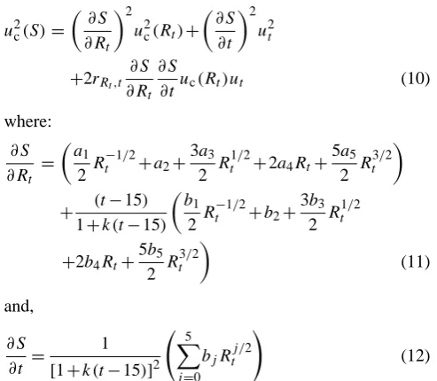
where: ∂S ∂Rt
=
a
1 2 R
−1/2
t +a2+ 3a3
2 R 1/2
t +2a4Rt+
5a5 2 R
3/2
t
+ (t−15)
1+k (t−15)
b
1 2R
−1/2
t +b2+ 3b3
2 R 1/2
t
+2b4Rt+
5b5 2 R
3/2
t
(11) and,
∂S ∂t =
1 [1+k (t−15)]2
5
X
j=0 bjRtj/2
!
(12)
Table 1 gives the values of uc(S)obtained with the GUM computation (0.00081) and with a Monte Carlo simulation (0.00085) for the salinityS=35. ForS=10, the same com-putations give 0.00023 and 0.00025 and forS=40: 0.00099 and 0.0011. These calculations show that relation (10) can be simplified because the contribution of the first term is largely superior to the contribution of the others, and it can be writ-ten as:
uc(S)≈
∂S ∂Rt
u
c
(Rt) (13)
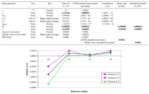
Table 1. Parameters of the input quantities used to compute the expanded uncertainty of Guildline Portasal salinometer forS=35, by the GUM and the Monte Carlo (M.C.) methods.
Input quantities Unit Pdf Value for GUM standard measurement Contribution Mean value Standard deviation
S=35 uncertainty toRt by M.C. by M.C.
t ◦C Normal 24 0.0010
rt None Normal 1.212266 0.000024 3.987E−10 K15 None Normal 0.99984 5.00E−06 2.500E−11
Gst mS cm−1 Right-angled triangle 52.0153 0.75E−04 0.000E+00
G mS cm−1 Right-angled triangle 52.0153 0.75E−04 0.000E+00
δkcell None Normal 1.21229 −8.51E−07 ∼4.931E−13
Rt None Normal 0.999862 0.000021 0.999848 0.000022 S None Normal 34.9950 0.00081 34.9940 0.00085 Linearity correction None Normal 0.0000 0.0001
Salinity value of the bottles None Right-angled triangle 0.0000 0.00024 PSS-78 fits None Normal 0.0000 0.0007
GUM expanded uncertainty: 0.0022
Monte Carlo expanded uncertainty: 0.0022
-0,0060 -0,0050 -0,0040 -0,0030 -0,0020 -0,0010 0,0000 0,0010
10 30 35 38
Reference salinity
S
a
li
n
it
y
e
rr
o
r
Portasal n°1
Portasal n°2
Portasal n°3
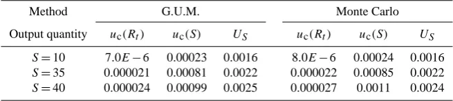
Figure n° 1: examples of linearity errors measured on three Portasal salinometers after
calibration with standard seawater bottles.
Fig. 1. Examples of linearity errors measured on three Portasal salinometers after calibration with standard seawater bottles.
made by OSIL on Portasal salinometers (see Fig. 1). Hard-ware corrections are difficult to make because linearity can be non-uniform in the range of measurements. So, salin-ity values must be corrected by linear relations on different sub-ranges. These corrections have a standard uncertaintyul
which is, at least, equal to the linear regression remainder or 0.0001.
Secondly, standard salinity bottles used for the calibration and linearization can show maximum salinity variations of 0.001, for 96 weeks of storage, according to Culkin and Rid-out (1998). Resulting from this available information we can assign a rectangular pdf to this uncertainty (usb)according to the GUM. The standard deviation of such a function leads us to expressusbas:usb=0.001/
√
3.
Thirdly, PSS-78 relations fits have a standard deviation which is of 0.0007 at atmospheric pressure, according to Perkin and Lewis (1980), and of 0.0015 if the pressure term Rpis different from 1. The pdf of this uncertainty (uPSS)can be considered as being Normal. In the case of salinometers, uPSS=0.0007.
ul,usb,uPSS anduc(S)being independent variables, the expanded uncertainty US on the salinity, expressed with a
coverage factor of 2 to obtain a level of confidence close to 95 %, can be written as:
US=2
q
uc(S)2+u2l+u2sb+u2PSS (14) Table 1 gives the values of US computed with the GUM
and Monte Carlo methods and it is the same whatever the method: US=0.0022 forS=35 for a Portasal salinometer.
Table 2 gives the values obtained forS=10 and 40. It ap-pears that the two methods give close results and that for 35 and 40 the expected uncertainty of 0.002 cannot be main-tained. The main error sources are the stability of the bath temperature, the linearity of the salinometer, the salinity of the bottles of standard seawater and the PSS-78 itself.
Table 2. Standard uncertainties ofRt andS, and expanded uncertainty on the corrected value ofS, calculated using the two methods for
three different salinities. These values do not take into account possible long term variations in KCl standard solutions used to adjust standard seawater bottles, or the limits of metrological standards in terms of long term traceability of the salinity.
Method G.U.M. Monte Carlo
Output quantity uc(Rt) uc(S) US uc(Rt) uc(S) US
S=10 7.0E−6 0.00023 0.0016 8.0E−6 0.00024 0.0016
S=35 0.000021 0.00081 0.0022 0.000022 0.00085 0.0022
S=40 0.000024 0.00099 0.0025 0.000027 0.0011 0.0024
Cref=RtrtC(35,15,0) (15)
where rt is given by the relation (3) and Rt is obtained
according to Fofonoff and Millard (1983), with a Newton-Raphson iteration and the formula:
Rt n+1=Rt n+(S−Sn)
∂S
∂Rt
−1
(16)
on condition that we calculate (∂S/∂Rt)with the first part of
the relation (11).
C(35, 15, 0) is a constant to which several values have been attributed. According to Culkin and Smith (1980), C(35,15,0)=42.914 mS cm−1 and according to Poisson (1980),C(35,15,0)=42.933 mS cm−1. A recent study pub-lished by a BIPM working group (CCQM pilot study P111) has attributed the value 42.9104 mS cm−1toC(35,15,0), af-ter inaf-ter-comparisons made by different metrology laborato-ries (Seitz et al., 2010). In fact, in the case of CTD conduc-tivity sensor calibrations, it does not matter which value is used, provided that the same value is used during data reduc-tion and reference conductivity computareduc-tions. Most recent instruments are referenced to 42.914, so, let us take this value in uncertainty calculations,C(35,15,0)being considered as a constant.
The value ofRt obtained with the relation (16), depends
essentially on S which is measured by a laboratory sali-nometer andrt depends ont. So, we can write thatuRt= (∂Rt/∂S)u(S) and urt =(∂rt/∂t )ut. However, the
com-putation of the numerical values of Rt and rt for
differ-ent temperatures between 0 and 40◦C, shows that the cor-relation coefficient rRt,rt is not equal to zero. For p=0
andS=35,rRt,rt=0.53, for S=40,rRt,rt=0.56 and for S=10,rRt,rt=0.964. So,Rt andrt cannot be considered as
two independent variables, and the combined uncertainty of Crefis given by:
uCref=C (35,15,0)
"
rt2
∂R
t ∂S
2
u2(S)+Rt2
∂r
t ∂t
2
u2t
+R
∂R
t
∂S ∂rt
∂t
u(S)utrRt,rt
1/2
(17)
(∂S/∂Rt)can be calculated with the main part of the
rela-tion (11) andu(S)=US/2;US being calculated with the
re-lation (14).
(∂rt/∂t) is the polynomial of the relation (8), but in
rela-tion (17)ut is the uncertainty of the reference temperatures
measured during the calibration of the conductivity sensor. ut depends on reference thermometer calibration
uncertain-ties at fixed ITS-90 points, but also, on the drift of this ther-mometer between two calibrations, as well as on its self-heating during the measurements and on the stability and uniformity of the calibration bath temperature.
In 2002, the BIPM published a guide (Fellmuth et al., 2002) about uncertainty budgets for the calibration of stan-dard platinum reference thermometers (SPRT) at the fixed ITS-90 points. It takes into account the calibration uncer-tainties of the fixed points cells themselves, the making of the points, the self-heating errors and the repeatability of the sensors but also, the non-uniqueness of the scale. This un-certainty budget can be applied to other kinds of reference thermometers, such as Sea Bird Electronics SBE 35, which are used to calibrate CTD profilers at sea. In the best case, it leads to a combined standard uncertainty of 0.39 mK. This value is largely dependent on the uncertainty of the tempera-ture assigned to the reference cells, which is given by the pri-mary calibration laboratories. For example, a gallium melt-ing point cell calibrated in the UK with a UKAS certificate will have an expanded uncertainty of±0.25 mK. The same calibration made in France by the National Calibration Lab-oratory (LNE) under the same procedure, with a COFRAC certificate, will be given with an expanded uncertainty of 1.2 mK. This will give a combined standard uncertainty of 0.7 mK.
0 5 10 15 20 25 30
0.00 to 0.01
0.01 to 0.02
0.02 to 0.03
0.03 to 0.04
0.04 to 0.05
0.05 to 0.06
0.06 to 0.07
> 0.07
mS/cm %
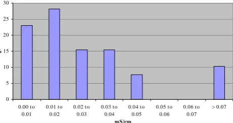
Figure 2: annual drift statistics of the 32 thermosalinographs SBE 21 of the French
operational oceanography project Coriolis. Only 23 % of them show annual shifts less than
0.01 mS/cm but 51 % have annual shifts less than 0.02 mS/cm. This shows how much drift
there can be in conductivity cells submitted to strong environmental conditions. Fig. 2. Annual drift statistics of the 32 thermosalinographs SBE 21
of the French operational oceanography project Coriolis. Only 23 % of them show annual shifts less than 0.01 mS cm−1but 51 % have annual shifts less than 0.02 mS cm−1. This shows how much drift there can be in conductivity cells submitted to strong environmental conditions.
Then, the reference temperature’s combined uncertainty can be, in the best case: ut=0.54 mK. With a COFRAC
certificate on the fixed points cell:ut=0.80 mK.
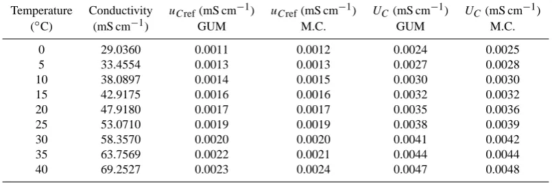
Table 3 shows values ofuCrefcalculated for different tem-peratures, conductivities andS=35, withut=0.54 mK and u(S)=0.0011. Monte Carlo assessments and GUM calcu-lations give very close values, and it appears that, even with a very good measure of temperature, standard combined un-certainties of reference conductivities are close or superior to 0.002 mS cm−1 for high conductivity values. It also ap-pears that the cross-term of the expression (17) cannot be neglected.
Conductivity sensors of CTD floats or profilers are lin-earized with polynomials before being used at sea. So, to find out what the uncertainty of the measured conductivity is, we must add touCref, the square sum of the polynomial residualsuCl and the uncertainty on the CTD sensor
read-ings which can be assessed by the repeatability of the sensor measurements uCr. uCref, uCl anduCr being independent
variables, the expanded uncertaintyUC of the conductivity
values measured at sea (with a level of confidence close to 95 %), can be expressed as:
UC=2
q
u2Cref+u2Cl+u2Cr (18)
An estimate of the annual drift of the sensor could be added to this sum to have a real idea of the uncertainty of conduc-tivity measurements. This error source has very variable am-plitudes because it depends on the environment and the du-ration of measurements but also on the use of anti-fouling devices or on the regularity of sensor cleaning. It varies from 0.001 mS cm−1yr−1to several 0.01 mS cm−1yr−1. In order to illustrate this variation, Fig. 2 shows the statis-tics of 32 thermosalinographs SBE 21 calibrated yearly at the SHOM calibration laboratory since 2003, in the frame-work of the French operational oceanography project
Cori-olis, which contributes to the ARGO and GODAE experi-ences. This figure shows the drifts of conductivity cells sub-mitted to strong environmental conditions.
So, in order to assess the value ofUC, we will just consider
the initial uncertainty of the measurements. A usual value for uClis 0.0002 mS cm−1and, as an example, we can take the
repeatability of a Sea Bird Electronics SBE 4 conductivity cell, which can be considered as equivalent to their resolution oruCr=0.0004 mS cm−1, and it follows a Normal law. UC
has been calculated with these values and the results are also given in Table 3. It appears that expanded uncertainties of conductivity measured values, obtained with the two meth-ods, are largely greater than 0.002 mS cm−1, particularly for high conductivity values.
4 Uncertainties on salinities calculated from CTD sensors data
Salinity is calculated with relation (9) when data are mea-sured with CTD sensors, but the pressure effect must be taken into account and in this case,Rtis obtained with:
Rt= R rtRp
(19) In this relation,rt is given by the relation (3) and its
uncer-tainty by the relation (8), in whichut is the standard
uncer-tainty of the temperatures measured by the CTD sensor. Con-sidering the elements given in the previous paragraph about temperature calibration and the quality of the CTD’s temper-ature sensors,ut can be estimated to be equal to 0.001◦C (in
the best case). Ris the ratio: R= C (S,t,p)
C (35,15,0)) (20)
C(S,t,p)is the conductivity measured by the conductivity sensor. Its expanded uncertainty is given by the relation (18). C(35,15,0)is the constant whose value has been discussed in the previous paragraph. C(35,15,0)=42.914 mS cm−1 anduR=uC=UC/2, values ofUCbeing given in Table 3.
Rpis the coefficient for pressure effects correction. Rpis
given by: Rp=1+
p e1+e2p+e3p2
1+d1t+d2t2+(d3+d4t )R
(21) e1,e2,e3 and d1,d2,d3,d4 are constants whose values are given in Perkin and Lewis (1980). p andt are two inde-pendent quantities, but R is proportional to C(S,t,p) and strongly correlated tot. The calculation of the correlation co-efficientrR,t, with the temperature-conductivity data of
Ta-ble 3 givesrR,t=0,9995. Let us takerR,t≈1. In this case,
the combined standard uncertainty onRp(uRp)can be
writ-ten: u2R
p=
∂R
p
∂p
2
u2p+
∂R
p
∂t ut+ ∂Rp
∂R uR
2
Table 3. Standard combined uncertainties on reference conductivities (uCref), computed for different values of temperature, conductivity
and forS=35, and expanded uncertainty of conductivity values measured with linearized sensors (UC). UCanduCrefwere assessed with
the GUM and Monte Carlo Method (M.C.).
Temperature Conductivity uCref(mS cm−1) uCref(mS cm−1) UC(mS cm−1) UC(mS cm−1)
(◦C) (mS cm−1) GUM M.C. GUM M.C.
0 29.0360 0.0011 0.0012 0.0024 0.0025
5 33.4554 0.0013 0.0013 0.0027 0.0028
10 38.0897 0.0014 0.0015 0.0030 0.0030
15 42.9175 0.0016 0.0016 0.0032 0.0032
20 47.9180 0.0017 0.0017 0.0035 0.0036
25 53.0710 0.0019 0.0019 0.0038 0.0039
30 58.3570 0.0020 0.0020 0.0041 0.0042
35 63.7569 0.0022 0.0021 0.0044 0.0044
40 69.2527 0.0023 0.0024 0.0047 0.0048
The calculation of the sensitivity coefficients leads us to write the final relation:
uRp= (23)
h
e1+2e2p+3e3p2 2
u2p+ Rp−1 2
[(d1+2d2t+d4R)ut+(d3+d4t )uR]2
i1/2
1+d1t+d2t2+(d3+d4t )R
The value ofup, the standard uncertainty of pressure
mea-surements, remains to be found. Accuracy and precision of pressure sensors depend on their range of measurement. Pressure balances used to calibrate them, must undergo cor-rections for normal gravity, height difference with the sen-sor, thermal and pressure expansion of the piston and of the air-mass hydrostatic pressure difference. After that, the expanded uncertainty of a reference pressure given by an 8000 dbar balance is calculated by a relation of this kind: UPref=0.12+0.00013p (dbar) (24) If the repeatability of a 6000 dbar sensor (and its electron-ics) is 0.2 dbar, and that its residual temperature drift is also 0.2 dbar, then up=0.53 dbar at 6000 dbar or 0.34 dbar at
2000 dbar.
With these elements, the expression of the standard com-bined uncertainty onRt, obtained with relation (19) must still
be written. So, the GUM method applied to relation (19) leads us to write:
uc(Rt)2=
∂R
t ∂R
2
u2R+
∂R
t ∂Rp
2
u2R
p+
∂R
t ∂rt
2
u2rt
+2∂Rt ∂R
∂Rt ∂Rp
uRuRprR,Rp+2
∂Rt ∂rt
∂Rt ∂Rp
urtuRprrt,Rp
+2∂Rt ∂R
∂Rt ∂rt
uRurtrR,rt (25)
The development of the relation (25) gives: uc(Rt)=Rt
" uR
R
2
+
u
Rp
Rp
2
+
u
rt
rt
2
−2uR R
uRp
Rp rR,Rp
+2uRp Rp
urt
rt
rrt,Rp−2
uR R
urt
rt rR,rt
1/2
(26) The correlation coefficients of the variables R, Rt and rt
have been computed for the salinities S=10, 35, 38 and 40, with the numerical values of t, C and p displayed in Table 4. This gives: rR,Rp= −0.44,rR,rt=0.998≈1 and rRp,rt= −0.50, and shows that cross-terms cannot be
ne-glected. Moreover, neglecting this terms would increase the uncertainty estimate. For example, for t=2◦C, C=
33.038 mS cm−1andp=6000 dbar,uc(Rt)=5×10⁻⁴and uc(S)=0.0019, without the correlation terms, but with this termsuc(Rt)=1.4×10⁻⁵anduc(S)=0.0005! The uncer-tainties on practical salinity computations take advantage of the ratio expression of Rt, which reduces the effect of the
uncertainties of each of the input variables.
With the correlation coefficients given previously, rela-tion (26) can be simplified to give:
uc(Rt)=Rt
"
uR R−
urt
rt
2
+uRp Rp
u
Rp
Rp
+0.88uR R −
urt
rt
#1/2
(27) In fact, it is the standard uncertainty of the PSS-78 relations fits, given in Perkin and Lewis (1980), which increases the uncertainty inS significantly, particularly in the case when Rpvalue is different from 1:uPSSis then equal to 0.0015.
Then, in the case of CTD measurements, the expanded uncertainty in salinity computations can be assessed (with a level of confidence close to 95 %) by the relation:
US=2
q
uc(S)2+u2PSS (28)
whereuc(S)can be calculated with relations (13) and (26) or (27).
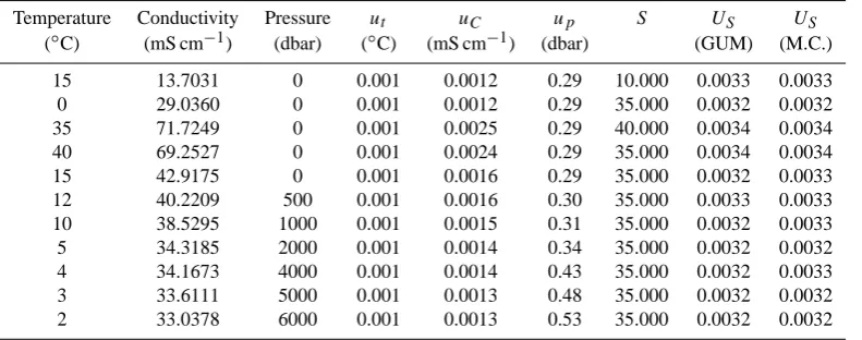
Table 4. Expanded combined uncertainties on salinity, computed with representative values of temperature, conductivity and pressure and
their combined standard uncertainties. Conductivity combined standard uncertaintiesuCcorrespond to the values found in table 3 and for
temperature, the standard uncertainty corresponds to the best case whenut=0.001◦C. Idem forup.
Temperature Conductivity Pressure ut uC up S US US
(◦C) (mS cm−1) (dbar) (◦C) (mS cm−1) (dbar) (GUM) (M.C.)
15 13.7031 0 0.001 0.0012 0.29 10.000 0.0033 0.0033
0 29.0360 0 0.001 0.0012 0.29 35.000 0.0032 0.0032
35 71.7249 0 0.001 0.0025 0.29 40.000 0.0034 0.0034
40 69.2527 0 0.001 0.0024 0.29 35.000 0.0034 0.0034
15 42.9175 0 0.001 0.0016 0.29 35.000 0.0032 0.0033
12 40.2209 500 0.001 0.0016 0.30 35.000 0.0033 0.0033
10 38.5295 1000 0.001 0.0015 0.31 35.000 0.0032 0.0033
5 34.3185 2000 0.001 0.0014 0.34 35.000 0.0032 0.0032
4 34.1673 4000 0.001 0.0014 0.43 35.000 0.0032 0.0033
3 33.6111 5000 0.001 0.0013 0.48 35.000 0.0032 0.0032
2 33.0378 6000 0.001 0.0013 0.53 35.000 0.0032 0.0032
(US=0.0034 on average). These results are greater by about
0.0014 than the 0.002 expected by the WOCE programme. More, this uncertainty assessment is valid only in areas where temperature and salinity gradients are low. When measurements are made in areas of strong temperature and (or) salinity gradients, the major errors in practical salinity measurements come from the ability to align the response times of temperature and conductivity sensors, even when data are corrected with manufacturers’ correction algorithms, as shown by Mensah et al. (2009). On average, errors up to 0.017 still persist for some measurements in strong salinity gradients and increase the uncertainty in practical salinity by as much, if they cannot be detected and corrected.
Lastly, we must not forget that practical salinity is only one way to approach the absolute salinity SA of seawater which is the real quantity to access thermodynamic proper-ties of the ocean and ocean-atmosphere interactions. There-fore, the fact that non-electrolyte components are not de-tected by conductivity sensors and that the seawater com-ponents ratio is not clearly known, leads to a difference of about 0.45±0.05 % betweenSandSAand to an uncertainty of 0.16 ppt in SA, even at S=35, as estimated by Jackett and McDougall (2006). Then, the expanded uncertainty of 0.0034 onS, as obtained with relation (28), can be consid-ered as largely sufficient and even insignificant in the assess-ment of the absolute salinity.
5 Conclusion
The uncertainties of practical salinity calculations have been assessed by two standardized independent methods: the GUM and Monte Carlo, in the case of salinities obtained with laboratory salinometers and in the case of CTD mea-surements after laboratory calibration of conductivity cells.
The two methods give coherent and very similar results. The 0.002 psu required initially by the WOCE program are ob-tained with difficulty, even in the case of laboratory sali-nometers. However, in the error budget, the part due to the PSS-78 relations fits is sometimes as significant as the in-strument’s. This is particularly the case with CTD measure-ments where correlations between theRtvariables contribute
mainly to decreasing the uncertainty onS, even when the ex-panded uncertainties of conductivity cell calibrations are for the most part in the order of 0.002 mS cm−1. The relations given in this publication and obtained with the normalized GUM method, allow a real analysis of uncertainty sources and they can be used in a general way to assess the uncer-tainty in conductivity cells calibrations or practical salinity calculations made with data from instruments having speci-fications different from the examples taken in Tables 1 to 4.
Appendix A
PSS 78 algorithm as defined in Fofonoff and Millard (1983)
pis expressed in dbar,tin◦C andCin S m−1
a1=0.0080,a2= −0.1692,a3=25.3851,a4=14.0941, a5= −7.0261,a6=2.7081
b1 = 0.0005, b2 = −0.0056, b3 = −0.0066, b4= −0.0375,b5=0.0636,b6= −0.0144
d1=3.426×10⁻², d2=4.464×10⁻⁴, d3=0.4215, d4= −3.107×10⁻³
e1 = 2.070 × 10⁻⁵, e2 = −6.370 ×10⁻¹⁰, e3 = 3.989×10⁻¹⁵
Probe:
R=C/4.2914
R1=c1+(c2+(c3+(c4+c5×t )×t )×t )×t
RP =1+((e1+(e2+e3×p)×p)×p)/(1+(d1+d2× t )×t+(d3+d4×t )×R)
Rt=R/(R1×RP)
Edited by: J. M. Huthnance
References
Bacon, S., Culkin, F., Higgs, N., and Ridout, P.: IAPSO Standard Seawater: definition of the uncertainty in the calibration proce-dure and stability of recent batches, J. Atmos. Oceanic Technol., 24, 1785–1799, 2007.
BIPM: Evaluation of measurement data – Supplement 1 to the Guide to the expression of uncertainty in measurement – Prop-agation of distributions using a Monte Carlo method, JCGM YYY:2006, 2006.
BIPM: Evaluation of measurement data – Guide to the expression of uncertainty in measurement, JCGM 100:2008, GUM 1995 with minor corrections, 2008.
Culkin, F. and Ridout, P. S.: Stability of IAPSO Standard Seawater, J. Atmos. Oceanic Technol., 15, 1072–1075, 1998.
Culkin, F. and Smith, N.: Determination of the concentration of potassium chloride solution having the same electrical conduc-tivity, at 15◦C and infinite frequency, as standard seawater of salinity 35,000 ‰, (Chlorinity 19.37394 %), IEEE J. Oceanic Eng., OE-5, no. 1, 22–23, 1980.
Fellmuth, B., Fisher, J., and Tegeler, E.: Uncertainty budgets for characteristics of SPRTs calibrated according to the ITS-90, BIPM, CCT/01-02, 2002.
Fofonoff, N. P. and Millard, R. C.: Algorithms for computation of fundamental properties of seawater, Unesco technical paper in marine science 44, 1983.
Jackett, D. R. and McDougall, T. J.: Algorithms for density, po-tential temperature, conservative temperature and the freezing temperature of seawater, J. Atmos. Oceanic Technol., 23, 1709– 1728, 2006.
Kawano, T., Aoyama, M., and Takatsuki, M.: Inconsistency in the conductivity of standard potassium chloride solutions made from different high-quality reagents, Deep Sea Res. Part. I, 52, 389– 396, 2005.
Lueck, R. G.: Thermal inertia of conductivity cells: theory, J. At-mos. Oceanic Technol., 7, 741–755, 1990.
Mensah, V., Le Menn, M., and Morel, Y.: Thermal mass correction for the evaluation of salinity, J. Atmos. Oceanic Technol., 26, 665–672, 2009.
Perkin, R. G. and Lewis, E. L.: The Practical Salinity Scale 1978: Fitting the Data, IEEE J. Oceanic Eng., OE-5, no. 1, 9–16, 1980. Poisson, A.: Conductivity/Salinity/Temperature relationship of di-luted and concentrated standard seawater, IEEE J. Oceanic Eng., OE-5, no. 1, 41–50, 1980.
Saunders, P. M., Mahrt, K.-H., and Williams, R. T.: Standard and Laboratory Calibration, WHP Operations and Methods, 1991. Seitz, S., Spitzer, P., and Brown, R. J. C.: Consistency of
practi-cal salinity measurements traceable to primary conductivity stan-dards: Euromet project 918, Accreditation and Quality Assur-ance, 13, 601–605, 2008.
Seitz, S., Spitzer, P., and Brown, R. J. C.: CCGM-P111 study on traceable determination of practical salinity and mass fraction of major seawater components, Accred. Qual. Assur., 15, 9–17, 2010.