Parallel and perpendicular cascades in solar wind turbulence

(1)

SRef-ID: 1607-7946/npg/2005-12-299 European Geosciences Union

Nonlinear Processes

in Geophysics

Parallel and perpendicular cascades in solar wind turbulence

S. Oughton1and W. H. Matthaeus2

1_{Department of Mathematics, University of Waikato, Hamilton, New Zealand} 2_{Bartol Research Institute, University of Delaware, Newark, DE 19716, USA}

Received: 27 September 2004 – Revised: 10 February 2005 – Accepted: 12 February 2005 – Published: 17 February 2005 Part of Special Issue “Nonlinear processes in solar-terrestrial physics and dynamics of Earth-Ocean-System”

Abstract. MHD-scale fluctuations in the velocity, magnetic,

and density fields of the solar wind are routinely observed. The evolution of these fluctuations, as they are transported ra-dially outwards by the solar wind, is believed to involve both wave and turbulence processes. The presence of an average magnetic field has important implications for the anisotropy of the fluctuations and the nature of the turbulent wavenum-ber cascades in the directions parallel and perpendicular to this field. In particular, if the ratio of the rms magnetic fluc-tuation strength to the mean field is small, then the paral-lel wavenumber cascade is expected to be weak and there are difficulties in obtaining a cascade in frequency. The lat-ter has been invoked in order to explain the heating of solar wind fluctuations (above adiabatic levels) via energy transfer to scales where ion-cyclotron damping can occur.

Following a brief review of classical hydrodynamic and magnetohydrodynamic (MHD) cascade theories, we discuss the distinct nature of parallel and perpendicular cascades and their roles in the evolution of solar wind fluctuations.

1 Introduction

The solar wind exhibits fluctuations in the magnetic field, plasma velocity, and density over a broad range of length and time scales, as was suggested by Parker (1958) in con-nection with his original model for the (large-scale) solar wind. Many of these fluctuations occur at magnetohydrody-namic (MHD) scales, although dissipative processes almost certainly require account to be taken of plasma-scale or ki-netic effects.

The nature of the MHD-scale fluctuations is a question of some interest. Analysis of even the earliest observations pro-vided evidence for the presence of both waves and turbulence (e.g. Coleman, 1968; Belcher and Davis, 1971), and it now seems clear that Alfv´en waves and turbulence are pervasive Correspondence to: S. Oughton

(seano@waikato.ac.nz)

features of the interplanetary medium, although their relative importance has yet to be fully determined (e.g. Matthaeus et al., 1995; Goldstein et al., 1995; Tu and Marsch, 1995; Veltri and Malara, 1997; Velli et al., 2003).

Both the wave and turbulence dynamics are influenced by the preferred directions present in the interplanetary medium. These include the radial expansion direction and the mean magnetic field. In particular, there is evidence for spec-tral and/or variance anisotropy with respect to one or both of these preferred directions (e.g. Belcher and Davis, 1971; Klein et al., 1991; Matthaeus et al., 1990, 1996; Bieber et al., 1996; Carbone et al., 1995; Horbury et al., 1995).

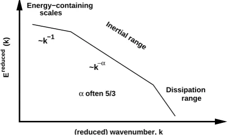
As is well-known, the wavenumber energy spectrum for a turbulent fluid can be characterized in terms of three dif-ferent wavenumber ranges, namely the energy-containing, inertial, and dissipation ranges (e.g. Lesieur, 1990; Frisch, 1995; Biskamp, 2003). Figure 1 shows a schematic solar wind spectrum. In the classical view of turbulence, energy is transferred from the energy-containing scales to the dissipa-tion range scales not directly, but rather via passage through the inertial range “pipeline”. In other words, the energy cas-cades from wavenumber to (somewhat) larger wavenumber until it reaches scales where the direct effects of dissipation are important. The inertial range dynamics is self-similar which yields a powerlaw energy spectrum there, for large enough Reynolds numbers. The question then arises, what can be determined about the nature of solar wind fluctuations from observable quantities like the energy spectrum?

(2)

3002 S. Oughton and W. H. Matthaeus: Parallel and perpendicular cascadesS. Oughton and W. H. Matthaeus: Parallel and perpendicular cascades

range

E (k)

reduced

scales

Dissipation

(reduced) wavenumber, k

~k −1

−α

~k

Energy−containing

Inertial range

often 5/3 α

Fig. 1. Schematic energy spectrum for the fluctuation energy of the solar wind. The energy-containing, inertial, and dissipation ranges are indicated. Note the powerlaw nature of the spectrum in the in-ertial range.

siders observational evidence for the existence of two distinct types of fluctuations in the solar wind. In Sect. 4 a simple model is employed to show that slopes of 5/3 can be com-mon even when there is a non-5/3 component. The paper closes with a short summary.

The basic notation employed is standard, with and

re-spectively the fluctuating velocity and magnetic fields, the

mass density, and the Fourier wavevector conjugate to the

spatial position vector . Magnetic fields are assumed to be

measured in Alfv´en speed units, obtained starting from labo-ratory units by letting

.

2 MHD Cascade Theory

In some ways the physics of (Navier–Stokes) turbulence is more about lengthscales then timescales, since the funda-mental action of the nonlinear terms is to transfer excita-tion between lengthscales. Thinking in Fourier space, this could be rephrased as the primacy of the wavevector spec-trum over the frequency specspec-trum. Of course, each length-scale (or wavevector) has one or more timelength-scales associated with it, so that there is also an inherent transfer of energy between timescales. In particular, the rates of energy trans-fer are of importance, helping to determine cascade proper-ties and the shape of the energy spectrum. Indeed, as we review below, Kolmogorov theory can be reformulated in terms of such timescales, showing that it is the triple cor-relation timescale,, that determines the slope of the

en-ergy spectrum in the inertial range. In MHD turbulence, as contrasted with Navier–Stokes, the situation is further com-plicated by the presence of Alfv´en waves and their associated timescales.

In the subsections below we first review Kolmogorov the-ory for hydrodynamics and the Iroshnikov–Kraichnan (IK) extension of it to incompressible MHD, and then summa-rize work addressing the primary shortcoming of the IK

ap-proach, namely the assumption of isotropy. Subsections on compressible anisotropy results and forcing/inhomogeneity related timescales round out the section.

2.1 Kolmogorov (hydrodynamic) phenomenology

Suppose that an incompressible Navier–Stokes fluid1 is forced isotropically at some set of large length and time scales so that a statistically steady turbulent flow is set up. The Kolmogorov (1941)!

form for the inertial range en-ergy spectrum can be obtained via dimensional analysis and the assumption that there is a range of lengthscales for which (i) direct viscous damping is negligible,2(ii) the energy flux at wavenumber , denoted"#$, depends only on local

quan-tities, namely and the spectrum%&$, and (iii) the flux of

energy through this range is in fact a constant. Also implicit is the assumption that the energy is distributed isotropically. Given this isotropic situation, it is convenient to work with the omni-directional (or angle-integrated) spectrum. This is defined by

%&$(' %

*)

+-,./10 (1)

where % 2)

is the modal energy spectrum and ./ the

differential solid angle. The total turbulence energy is

3

4

%&$5.6 , so that %78 is readily interpreted as the

en-ergy per wavenumber at .

Assuming that"98:&';=<>%&$@? , for constantsA andB ,

and employing the above assumptions then yields %&8:C'

"

,

D#

, to within an undeterminedEFHG- constant usually

called the Kolmogorov constant. For fuller discussion of hy-drodynamic turbulence see, for example, Batchelor (1970), Lesieur (1990), and Frisch (1995).

The Kolmogorov form can also be obtained somewhat more physically, by reformulating the approach to take ex-plicit account of the relevant ( -dependent) timescales. In

order to do so we first define these timescales.

There are (at least) three conceptually distinct timescales associated with each wavevector .

– The nonlinear time isIKJ> G

$5L6M:, whereL ,M is

approximately the kinetic energy per mass in wavevec-torsNO , and represents the timescale associated with

nonlinear modification ofL M .

– The triple correlation timescale P characterizes

the time separation over which third-order correlations (written symbolically asQRL:LLTSVU withL andLTS at

differ-ent times) tend to zero.

– The spectral transfer timescaleW is the time for a

significant fraction of the energy in wavevectors to

be transfered to other wavevectors. A common defini-tion is via (Obukhov, 1941)

.

.+X LT,M '

"9PY Z

L

,M

[WY\

(2)

1_{Meaning gravity, Coriolis force, etc. play no important role.} 2

Thus viscosity is not a relevant parameter in the inertial range. Fig. 1. Schematic energy spectrum for the fluctuation energy of the

solar wind. The energy-containing, inertial, and dissipation ranges are indicated. Note the powerlaw nature of the spectrum in the in-ertial range.

The paper is structured as follows. In the next section we review cascade theory for MHD turbulence. Section 3 con-siders observational evidence for the existence of two distinct types of fluctuations in the solar wind. In Sect. 4 a simple model is employed to show that slopes of 5/3 can be com-mon even when there is a non-5/3 component. The paper closes with a short summary.

The basic notation employed is standard, withvandb re-spectively the fluctuating velocity and magnetic fields,ρthe mass density, andkthe Fourier wavevector conjugate to the spatial position vectorx. Magnetic fields are assumed to be measured in Alfv´en speed units, obtained starting from labo-ratory units by lettingb→b/√4πρ.

2 MHD cascade theory

In some ways the physics of (Navier-Stokes) turbulence is more about lengthscales then timescales, since the funda-mental action of the nonlinear terms is to transfer excita-tion between lengthscales. Thinking in Fourier space, this could be rephrased as the primacy of the wavevector spec-trum over the frequency specspec-trum. Of course, each length-scale (or wavevector) has one or more timelength-scales associated with it, so that there is also an inherent transfer of energy between timescales. In particular, the rates of energy trans-fer are of importance, helping to determine cascade proper-ties and the shape of the energy spectrum. Indeed, as we review below, Kolmogorov theory can be reformulated in terms of such timescales, showing that it is the triple cor-relation timescale,τ3(k), that determines the slope of the en-ergy spectrum in the inertial range. In MHD turbulence, as contrasted with Navier–Stokes, the situation is further com-plicated by the presence of Alfv´en waves and their associated timescales.

In the subsections below we first review Kolmogorov the-ory for hydrodynamics and the Iroshnikov-Kraichnan (IK) extension of it to incompressible MHD, and then

summa-rize work addressing the primary shortcoming of the IK ap-proach, namely the assumption of isotropy. Subsections on compressible anisotropy results and forcing/inhomogeneity related timescales round out the section.

2.1 Kolmogorov (hydrodynamic) phenomenology

Suppose that an incompressible Navier-Stokes fluid1 is forced isotropically at some set of large length and time scales so that a statistically steady turbulent flow is set up. The Kolmogorov (1941)k−5/3form for the inertial range en-ergy spectrum can be obtained via dimensional analysis and the assumption that there is a range of lengthscales for which (i) direct viscous damping is negligible,2(ii) the energy flux at wavenumberk, denoted(k), depends only on local quan-tities, namelykand the spectrumE(k), and (iii) the flux of energy through this range is in fact a constant. Also implicit is the assumption that the energy is distributed isotropically. Given this isotropic situation, it is convenient to work with the omni-directional (or angle-integrated) spectrum. This is defined by

E(k)= Z

E3D(k) k2d, (1)

where E3D(k) is the modal energy spectrum and d the differential solid angle. The total turbulence energy is R∞

0 E(k)dk, so thatE(k)is readily interpreted as the energy per wavenumber atk.

Assuming that (k)=kαE(k)β, for constants α and

β, and employing the above assumptions then yields

E(k)=2/3k−5/3, to within an undeterminedO(1)constant usually called the Kolmogorov constant. For fuller discus-sion of hydrodynamic turbulence see, for example, Batchelor (1970); Lesieur (1990); Frisch (1995).

The Kolmogorov form can also be obtained somewhat more physically, by reformulating the approach to take ex-plicit account of the relevant (k-dependent) timescales. In order to do so we first define these timescales.

There are (at least) three conceptually distinct timescales associated with each wave vectork.

– The nonlinear time isτNL(k)≈1/(kuk), whereu2_kis ap-proximately the kinetic energy per mass in wavevectors ∼k, and represents the timescale associated with non-linear modification ofuk.

– The triple correlation timescale τ3(k) characterizes

the time separation over which third-order correlations (written symbolically ashuuu0iwithuandu0at differ-ent times) tend to zero.

– The spectral transfer timescaleτs(k)is the time for a

(3)

be transfered to other wavevectors. A common defini-tion is via (Obukhov, 1941)

d dtu

2

k = −(k)≈ −

u2_k τs

. (2)

Although in general functions of the full wavevector, insist-ing on isotropy means that the timescales, like the spectra themselves, are then functions ofk=|k|.

As noted by Kraichnan (1965), the energy flux should be proportional to the triple correlation timescale τ3(k). Assuming isotropy and matching the dimensions of

=τ3(k)kαE(k)βyields

=τ3(k)k4E(k)2, (3)

which might, mnemonically, be called the “2-3-4” rule. In isotropic hydrodynamics the three timescales are in fact equivalent: τs≈τ3≈τNL≈1/(kuk)≈1/[k

√

kE(k)], and sub-stitution into Eq. (3) yieldsE(k)=2/3k−5/3, as before.3 An advantage of this approach, however, is that it allows for more general situations in which the timescales differ, such as MHD which we discuss next.

2.2 Iroshnikov–Kraichnan (IK) phenomenology

Iroshnikov (1964) and Kraichnan (1965) independently sug-gested that for MHD turbulence with a strong large-scale magnetic field4 B0, a new timescale becomes important. This is the Alfv´en timescale,

τA(k)= 1 |k·B0|

= 1

k|B0cosθ|

, (4)

and is essentially the period of an Alfv´en wave with wavevec-tor k. Treating cosθ as approximately constant (i.e. ne-glecting the anisotropy ofτA), Kraichnan argued that since a strong B0 means that 1/(kB0) is very short, τA should provide the dominant contribution to the triple correlation time in MHD turbulence. Insertingτ3(k)=1/(kB0)in Eq. (3) yields the IK form

E(k)=pB0k−3/2. (5)

Physically, visualizing inertial range MHD turbulence as the interaction of counter-propagating5Alfv´en waves, it is clear that their large propagation speed limits the collision time of two such wave-packets to be∼τAτNL. The latter in-equality holds if the fluctuation amplitude at scale k, uk, is much smaller than the large-scale Alfv´en speedB0. Let

N (k)=τNL(k)/τA(k) be the number of wave periods in a 3_{The approximation}_u2

k≈kE(k)holds well whenE(k)is a

pow-erlaw (e.g. Lesieur, 1990, §6.4.1).

4_{The Iroshnikov and Kraichnan derivations are not identical. For}

example, Kraichnan considered incompressible MHD while Irosh-nikov considered the plasma beta≈1 compressible situation. Nei-ther author required that a dc field was present.

5_{In incompressible MHD, Alfv´en waves propagating in the same}

direction do not interact, either linearly or nonlinearly.

nonlinear time. In order to achieve the equivalent of a hy-drodynamic “collision” (i.e. a nonlinear interaction lasting for≈τNL),N2interactions of lengthτA are required, since the collisions are incoherent. Thusτs=N2τA=τ_NL2 /τAτNL, i.e. spectral transfer is slowed down by the presence of Alfv´en waves. Substituting this into =u2_k/τs(k)=const yields, as before, the IK formE(k)∼k−3/2.

Although well-regarded for many years, it is now recog-nized that there is an important problem with the IK ap-proach, namely the neglect of the intrinsic anisotropy of

τA(k)with respect toB0. There are many wavevectors for which k·B06≈kB0; in particular, modes with k⊥B0 have

τA(k)→∞, which is not a short timescale and so will not dominate the contribution toτ3for those ks. (Modes with

k·B0=0 are called the two-dimensional (2D) modes, while those withk·B0≈0 are the quasi-2D modes. See Oughton et al. (2004) for discussion of how smallk·B0needs to be.)

Thus the cascade in directions perpendicular and parallel toB0is likely to be different, engendering a non-isotropic modal spectrum. Consequently, the relevance of the IK phe-nomenology to MHD turbulence is probably more limited than was initially thought. In addition, the omni-directional spectrum does not have the clean interpretation pertaining in isotropic cases since excitations at different directions toB0 but with the same|k|are lumped together.

Models designed to take some account of this anisotropy have been proposed (Pouquet et al., 1976; Grappin et al., 1982; Matthaeus and Zhou, 1989). The key idea is that the rate of decorrelation of triples is

1

τ3 ≈ 1

τNL + 1

τA

, (6)

that is, the sum of the decorrelation rates from distinct phys-ical effects. In this case, decorrelation occurs due to the usual advective effects (rate∼1/τNL) and also via the limited time for which counter-propagating wave-packets are in con-tact. This simple model provides a bridge between the Kol-mogorov spectrum (τA→∞) and the IK spectrum (B0→∞) for the over-simplistic approximationk·B0≈kB0.

If instead the full anisotropicτA(k)is used in Eq. (6) and one tries to substitute this into a version of Eq. (3) based onE3D(k)rather thanE(k), there is an immediate problem since there are now (at least) two lengthscales present,k⊥and kk=kcosθ, which dimensional analysis cannot distinguish between.

Note that there is also another difference between MHD and hydrodynamic turbulence. The above phenomenologies all assume that the normalized cross helicity,

σc=

2hv·bi

hv2_{i + h}_b2_i, (7)

(4)

302 S. Oughton and W. H. Matthaeus: Parallel and perpendicular cascades 2.3 Anisotropy of the turbulence spectrum and its

conse-quences

When conditions are such that a large-scale mean magnetic fieldB0threads the plasma, the dynamics, including turbu-lence if it occurs, can be expected to respond to this preferred direction, frequently through development of anisotropy. This is seen even in the most basic models of linear MHD waves, where dispersion relations involve anisotropic terms like k·B0. In the simplest anisotropic model of fluctua-tion symmetry6 – the “slab model” – excited wavevectors

k lie alongB0 and the spectrum is one-dimensional. The slab model has been widely employed in cosmic ray scat-tering theory (Jokipii, 1966) and in interpretations of space-craft data (Belcher and Davis, 1971), and elsewhere, but it is undoubtedly too simple. For example, for incompressible MHD, the slab model allows no wave-wave couplings, and therefore no possibility of turbulence or a Kolmogorov-like cascade.

The overemphasis on the slab model in solar wind appli-cations probably derives from two unfortunate oversimpli-fications. First, the “Alfv´enic” fluctuations often observed in the solar wind (e.g. Belcher and Davis, 1971) are iden-tified by their high degree of correlation of the fluctuating components of the magnetic and velocity field; in turbulence terms these are high cross helicity states. Such fluctuations resemble wave normal modes of MHD for fluctuations prop-agating along the locally dc magnetic fieldB0; these might be assumed to obey a dispersion relationω=±k·B0for the frequencyω, and to have perfectly correlated (or anticorre-lated) velocity and magnetic perturbations, depending upon the sign of frequency. Second the fluctuation variances in each of the two directions transverse toB0, tend to be larger (by about a factor of five) than the parallel variance (Belcher and Davis, 1971; Klein et al., 1991; Horbury et al., 1995). The so-called “minimum variance direction” argument pro-ceeds to estimate the direction ofkas parallel to the direction of minimum variance, i.e.B0. Taken together, one concludes that the “turbulence” (which cannot be turbulence at all in the usual sense) has slab symmetry.

However, in strong MHD turbulence the cross helicity en-ters into the physics as well (e.g. Dobrowolny et al., 1980), and dispersion relations do not provide the time dependence in this case (i.e. there are many frequencies associated with eachk). In addition, the minimum variance argument, by it-self, cannot determine the direction ofk. Consider, for exam-ple, a total magnetic fieldB=(bx, by, B0)with fluctuations

bx=∂a(x, y)/∂y andby=−∂a(x, y)/∂x that are transverse

to the mean field. The wavevectors, however, are clearly perpendicular – not parallel – to B0. Since such fluctua-6_{The most frequent assumption, that of isotropy, postulates}

equal excitation in all wavevectorskwith the same|k|. Classical hydrodynamic turbulence theory (e.g. Batchelor, 1970) is almost entirely based on this assumption, and applications of it to the so-lar wind have sometimes made a tacit assumption of isotropy (e.g. Coleman, 1968; Tu et al., 1984).

tions have wavevectors lying in the plane perpendicular to the mean field, they are often called 2D fluctuations.

Besides being a counterexample to the minimum variance argument, 2D fluctuations form a kind of paradigm for turbu-lence, in much the same way that slab fluctuations represent the essence of MHD Alfv´en wave physics. 2D fluctuations havek·B0=0 and are of “zero frequency.”7 Therefore the Alfv´enic time decorrelation that entered into the discussion in Sect. 2.2 does not occur: the decorrelation of 2D fluc-tuations occurs without influence of the out-of-plane mag-netic fieldB0. Uninhibited by this wave propagation effect, 2D turbulence can be expected to be relatively stronger than other turbulence in which the nonlinear couplings decay in part due to propagation effects.8

Although 2D symmetry is itself another highly idealized case, it points towards families of symmetries that may in fact be relevant to MHD with a strong mean field. For example, it is well known in laboratory plasma studies (Zweben et al., 1979; Robinson and Rusbridge, 1971) that the correlation scales along the mean field are much longer than those per-pendicular to the mean field. This led to development of so-called “Reduced MHD” models (RMHD) which are “quasi-2D” in the sense that they have excited wavevectors only in a region ofk-space neark·B0≈0. They are also incompress-ible (or nearly so). Various derivations of RMHD (Kadomt-sev and Pogutse, 1974; Strauss, 1976; Montgomery, 1982; Zank and Matthaeus, 1992a), suggest how this kind of low-frequency quasi-2D dynamics may be the “leading-order” description of nonlinear evolution of MHD in the presence of a strong guide field (cf. Montgomery and Turner, 1981). The main point of the derivations of RMHD is that the strongest nonlinearities – and therefore the expectation of the strongest wavenumber cascade – will occur in regions ofk-space for which the nonlinear time is less than the Alfv´en time, i.e.

τNL(k)≤τA(k).

An interesting and recurring topic has been the study of the boundaries of applicability of the RMHD model. Mont-gomery (1982) noted that strong anisotropy of spectral trans-fer leads to “freezing out” of parallel spectral transtrans-fer, so thatkk no longer increases – in this limit there is no paral-lel cascade at all. Higdon (1984) recognized that quasi-2D turbulence confined within a dynamically determined region ink-space would have, in steady-state, a distinctive bound-ary shape in which the maximum (or, typical) excitedk⊥is related to the maximum excited kk. Later this was elabo-rated upon by Goldreich and Sridhar (1995, 1997) who made use of these ideas to note that the marginal condition of

τNL(k)=τA(k)would take on the powerlaw formk⊥∼k 3/2 k for steady MHD turbulence with ak−5/3_{inertial range} (Hig-don also obtained this scaling). They refer to this as a “criti-7 _{Here frequency means wave frequency, not a general (e.g.}

Fourier) decomposition of the time dependence.

8_{Propagation effects can enter the physics of the 2D turbulence}

(5)

k k

0

B δ λu

NL

(b) (a)

µ·¶¸ ~¹ Hydro−like

fluctuations

Non−hydrolike fluctuations

Hydrolike

τ

Non−Hydrolike (k)

A τ

= (k)

Fig. 2. (a) Partitioning of« -space on the basis of whether the

nonlinear time at« is less than the (nominal) wave period there: º¼»D½

P«>Y¾

¿

º5À

P«ª. The region where this holds defines the

“hydro-like region,” wherein nonlinear effects have primacy. Fluctuations in this region are not well described as waves. Conversely, outside the hydrolike region wave effects are of importance.

(b) Indication of the strength and direction of spectral transfer at selected points in« -space. Within the hydrolike region the transfer

is roughly isotropic and analogous to the hydrodynamic situation. Outside this region, parallel transfer is weak, perhaps exponentially so, while perpendicular transfer is still strong due to the resonant transfer mediated by the hydrolike modes. (After Oughton et al. (2004)).

fined in this way. This leads to an examination of “high-frequency” or non-RMHD couplings (see below).

Building on the critical balance concept, Cho et al. (2002) proposed a specific model for the (axisymmetric) energy spectrum of strong9_{MHD turbulence:}

%&8

0+[NÁ >Â

4

ÃÄÅ

]ÆDÇ]

8[Ç

,

0 (8)

where Ç is a characteristic lengthscale for the

energy-containing range. This model spectrum is valid for wavevec-tors above the energy-containing range and has the advantage that it falls off strongly with increasing]ÆD] while retaining

a strong perpendicular cascade. As stressed by Cho et al. (2002), it is not a unique choice, being postulated rather than derived. Nonetheless, it does provide a good fit to the simu-lation data they report on.

2.3.1 Dynamical appearance of quasi-2D turbulence A crucial test of whether RMHD10 models are indeed cen-tral in low-compressibility MHD turbulence is whether an initially isotropic spectral state will evolve into a state that becomes more like that envisioned in RMHD. For the case

9_{Meaning the turbulent energy is approximately equal to the}

en-ergy in the mean field.

10

Hereafter we often use RMHD, quasi-2D, and hydrolike as (near) synonyms. However, there are differences in their defini-tions. For example, RMHD fluctuations are necessarily of small amplitude relative to the mean field, whereas this need not be true for quasi-2D or hydrolike fluctuations. See, for example, Appendix B of Oughton et al. (2004).

thate

4

is a dc field, this was investigated numerically in incompressible 2D (Shebalin et al., 1983; Grappin, 1986) and later in 3D (Carbone and Veltri, 1990; Oughton et al., 1994; Matthaeus et al., 1996), with consistent results. See also Bondeson (1985). The basic conclusion is that spectral transfer of energy proceeds more rapidly into wavevectors perpendicular toe

4

. Wavevectors parallel to the mean field that are initially unpopulated remain relatively unpopulated because spectral transfer parallel toe

4

is weak. This can be understood on the basis of resonance arguments, as was first noted by Shebalin et al. (1983).11

The basic physics of the Shebalin et al. (1983) picture is correct, and there is evidence that it is valid in 3D as well as driven and slightly compressible low Mach number MHD (Matthaeus et al., 1996, 1998; Galtier et al., 2001). How-ever, Kinney and McWilliams (1998) made the very impor-tant observation that the preference for perpendicular spec-tral transfer extends to modes beyond those that fall into the RMHD category. Put differently, the propagation ef-fect is generally very strong for modes that are not in the RMHD segment of -space, except for those couplings that

are resonant in the sense of Shebalin et al. Even high-frequency, wave-like Fourier modes can engage in certain “zero-frequency” couplings, namely those catalyzed by the quasi-2D (or RMHD) modes that form one arm of their res-onant triads. Such couplings increase the of the

high-frequency modes, but leave the energy unchanged in the participating RMHD modes (e.g. Kinney and McWilliams, 1998; Matthaeus et al., 1998; Oughton et al., 1998, 2004). See Fig. 2b.

In order to quantify the weakness of the parallel cascade one can use simulation data to obtain mean wavenumbers computed parallel and perpendicular to an imposed dc mag-netic field (assumed parallel to the È axis). We define the

mean-square perpendicular wavenumber by

Q$-,

UÊÉ'

M

,

]Ë>6Ì05Í$]

,

M

]Ë6P 0 Í H]

,

0 (9)

with an analogous definition for its parallel counterpart,

QH ,Í

UÉ . Note that a weighting function is used, in this case

the electric current density Ë6, although any other

rele-vant field could have been employed, e.g., or . Weighting

withË emphasizes structure at smaller scales as compared

to weighting with . The summations are over all excited wavevectors.

Figure 3 shows the evolution of these (Ë -weighted) mean

wavenumbers, as determined from a set of unforced

pseu-11

Nonlinear interactions in incompressible MHD involve triads of wavevectors satisfying«¨ÎYÏ_«ÑÐTÒ}«

z

. For strong³ ´

, the most effective couplings are those triads that also satisfy a (wave) fre-quency matching condition. Only oppositely propagating fluctua-tions interact, so all interacting resonant triads of Fourier modes have at least one member that satisfies«>Ó-Ô

³ ´

ÏÕ (Shebalin et al.,

1983). Necessarily, the other two then have the same«Ö . Therefore

resonant spectral transfer will tend to increase~#× but not~ Ö.

Fig. 2. (a) Partitioning of k-space on the basis of whether the nonlinear time atk is less than the (nominal) wave period there: τNL(k)<∼τA(k). The region where this holds defines the “hydro-like region”, wherein nonlinear effects have primacy. Fluctuations in this region are not well described as waves. Conversely, outside the hydrolike region wave effects are of importance. (b) Indication of the strength and direction of spectral transfer at selected points in k-space. Within the hydrolike region the transfer is roughly isotropic and analogous to the hydrodynamic situation. Outside this region, parallel transfer is weak, perhaps exponentially so, while perpendicular transfer is still strong due to the resonant transfer me-diated by the hydrolike modes (after Oughton et al., 2004).

cally balanced” cascade (Fig. 2a). While this estimate seems to be reasonably accurate for initial conditions and/or forc-ing restricted to lie within the RMHD region (Maron and Goldreich, 2001; Cho et al., 2002), one may be faced with applications in which the fluctuations are not confined in this way. This leads to an examination of “high-frequency” or non-RMHD couplings (see below).

Building on the critical balance concept, Cho et al. (2002) proposed a specific model for the (axisymmetric) energy spectrum of strong9MHD turbulence:

E(k⊥, kk)∼k −10/3 ⊥ exp

− |kkL|

(k⊥L)2/3

, (8)

where L is a characteristic lengthscale for the energy-containing range. This model spectrum is valid for wavevec-tors above the energy-containing range and has the advantage that it falls off strongly with increasing|kk|while retaining a strong perpendicular cascade. As stressed by Cho et al. (2002), it is not a unique choice, being postulated rather than derived. Nonetheless, it does provide a good fit to the simu-lation data they report on.

2.3.1 Dynamical appearance of quasi-2D turbulence A crucial test of whether RMHD10 models are indeed cen-tral in low-compressibility MHD turbulence is whether an 9_{Meaning the turbulent energy is approximately equal to the}

energy in the mean field.

10 _{Hereafter we often use RMHD, quasi-2D, and hydrolike as}

(near) synonyms. However, there are differences in their definitions. For example, RMHD fluctuations are necessarily of small amplitude relative to the mean field, whereas this need not be true for quasi-2D or hydrolike fluctuations. See, for example, Appendix B of Oughton et al. (2004).

initially isotropic spectral state will evolve into a state that becomes more like that envisioned in RMHD. For the case that B0 is a dc field, this was investigated numerically in incompressible 2D (Shebalin et al., 1983; Grappin, 1986) and later in 3D (Carbone and Veltri, 1990; Oughton et al., 1994; Matthaeus et al., 1996), with consistent results. See also Bondeson (1985). The basic conclusion is that spectral transfer of energy proceeds more rapidly into wavevectors perpendicular toB0. Wavevectors parallel to the mean field that are initially unpopulated remain relatively unpopulated because spectral transfer parallel toB0is weak. This can be understood on the basis of resonance arguments, as was first noted by Shebalin et al. (1983).11

The basic physics of the Shebalin et al. (1983) picture is correct, and there is evidence that it is valid in 3D as well as driven and slightly compressible low Mach number MHD (Matthaeus et al., 1996, 1998; Galtier et al., 2001). However, Kinney and McWilliams (1998) made the very important ob-servation that the preference for perpendicular spectral trans-fer extends to modes beyond those that fall into the RMHD category. Put differently, the propagation effect is generally very strong for modes that are not in the RMHD segment of k-space, except for those couplings that are resonant in the sense of Shebalin et al. Even high-frequency, wave-like Fourier modes can engage in certain “zero-frequency” cou-plings, namely those catalyzed by the quasi-2D (or RMHD) modes that form one arm of their resonant triads. Such cou-plings increase thek⊥of the high-frequency modes, but leave the energy unchanged in the participating RMHD modes (e.g. Kinney and McWilliams, 1998; Matthaeus et al., 1998; Oughton et al., 1998, 2004). See Fig. 2b.

In order to quantify the weakness of the parallel cascade one can use simulation data to obtain mean wavenumbers computed parallel and perpendicular to an imposed dc mag-netic field (assumed parallel to thez axis). We define the mean-square perpendicular wavenumber by

hk⊥2ij =

P

kk⊥2|j(k⊥, kz)|2 P

k|j(k⊥, kz)|2

, (9)

with an analogous definition for its parallel counterpart, hk_z2i_j. Note that a weighting function is used, in this case the electric current density j(k), although any other rele-vant field could have been employed, e.g.vorb. Weighting withj emphasizes structure at smaller scales as compared to weighting withb. The summations are over all excited wavevectors.

Figure 3 shows the evolution of these (j-weighted) mean wavenumbers, as determined from a set of unforced pseu-11_{Nonlinear interactions in incompressible MHD involve triads}

(6)

304 S. Oughton and W. H. Matthaeus: Parallel and perpendicular cascades

B0= 0.5

0 Ø 1 Ù 2 Ú 3 Û 4 Ü 5 Ý TimeÞ 0 10 20 30

B0= 1.0

0 Ø 1 Ù 2 Ú 3 Û 4 Ü 5 Ý TimeÞ 0 10 20 30

B0= 3.0

0 Ø 1 Ù 2 Ú 3 Û 4 Ü 5 Ý Time 0 10 20 30

B0= 8.0

0 Ø 1 Ù 2 Ú 3 Û 4 Ü 5 Ý Time 0 10 20 30 <k ß ⊥>

<kz>

Fig. 3. Evolution of the average parallel and perpendicular wavenumbers for[àá

Î

incompressible simulations for several

val-ues of dc field strength,â

´

. The mean wavenumbers are rms values with a weighting of ¬ãDP«¨$¬äz at each scale; see Eq. (9). Initial

con-ditions for the simulations were identical, with the excited modes band-limited between¬«¬=Ï 4–20, having gaussian random phases,

and an Alfv´en ratio of unity. Theâ

´

ÏÕ case is not shown, but has

the two curves essentially overlain, as is to be expected for isotropy.

dospectral simulations.12 _{Each panel in the figure is for} a different value of the dc field strength, where the initial Reynolds numbers (å

- ) and and fields are identical for all runs. The trend towards “freeze-out” of the parallel cascade with increasingk

4

is clear. Indeed, saturation occurs for k

4}æ

ç

(Shebalin et al., 1983). This is to be contrasted with the behavior of Q$

,

U, which indicates that perpendic-ular transfer is still strong, although reducing somewhat with increasing k

4

(perhaps due mostly to the modest Reynolds numbers employed).

Keeping in mind the expectation that physical processes tend to be local, rather than depending on conditions “at infinity,” one might ask to what extent these results de-pend upon the uniformity of the mean magnetic field. One would expect that a strong magnetic field that varied on very large length scales would act, with regard to development of anisotropy, in almost the same way as a uniform dc field. This issue was addressed by Cho and Vishniac (2000) and Milano et al. (2001), who asked whether -space correlation statistics were anisotropic relative to the local magnetic field. Although their approaches were somewhat different, in each case second-order structure functions were used, and the re-sults were consistent with the above picture of the anisotropic development of gradients relative to the mean magnetic field. One can summarize the results as follows. Consider the second-order structure functions èCRéj'QH] T

é6ê ë 5 6Ì$] ,

U , where ê

ë

is a unit vector along the local magnetic

12_{To make the comparison with} ì8~

z

í[î fair, Fig. 3 actually plots

ì8~

z

×

î8ï

à , since there are two independent directions in the

perpen-dicular plane.

field, and èð§éC'ñQH] 6P

éTê ë ð TPÌH] ,

U where ê

ë

is a unit vector in any direction perpendicular to the magnetic field. Both studies are consistent with the statement that

èÌ§éÑòÁèCRé. This implies that the variation of the fluctu-ations perpendicular to the local magnetic field is of smaller scale compared to that along it. One might call this “cor-relation anisotropy” and it is the -space, local, version of the spectral anisotropy discussed above. Analyses of spec-tra and/or mean wavenumbers computed relative to the local mean field have also been performed (Maron and Goldreich, 2001; Cho et al., 2002; Muller et al., 2003). For the most part these support the[±Nå

,

scaling. It is reassuring to find that the physics of the development of anisotropy is, in the end, local.

Studies have also shown that propagation-induced spectral (and correlation) anisotropy is a property of incompressible and nearly incompressible MHD. For example, Matthaeus et al. (1996) found, with strong k

4

, that the solenoidal

(óvhDô'õ ) part of the velocity field exhibits spectral

anisotropy, while the longitudinal part (óåh[

' ) remains isotropically distributed in -space. This was confirmed later by Cho and Lazarian (2002), at higher resolution. Evidently this is due to the fact that suppression of spectral transfer is mainly associated with Alfv´enic fluctuations, which have the anisotropic dispersion relation;'ö°h

e

4

. Interest-ingly, one can arrive at a complementary result by consider-ing the asymptotic low Mach number limit of nearly incom-pressible MHD at varying plasma beta (Zank and Matthaeus, 1993). Therein, a regularized asymptotic expansion of the compressible MHD equations is carried out, and the con-ditions necessary to attain the incompressible limit investi-gated. A main conclusion, for order one or low plasma beta, is that the limit to incompressibility can occur only if the ex-cited wavevectors become arranged so that ó s óð for the solenoidal part of the velocity, and also for the magnetic fluctuations. Departures from this ordering occur atEF$÷ùø¼, where ÷ùø is the turbulent Mach number. This reinforces, from an entirely different perspective, the association of per-pendicular spectral (or correlation) anisotropy with the in-compressive motions of MHD turbulence.

A consistent conclusion emerges: provided that the turbu-lence is incompressible or nearly incompressible, MHD tur-bulence tends to produce gradients perpendicular to a strong magnetic field faster than it produces gradients along the same magnetic field. Generically, this is a consequence of the suppression of parallel spectral transfer by the Alfv´en wave propagation effect. Further physical insight is gained from deeper examination of several special cases.

2.3.2 Weak turbulence

We mentioned earlier that the high-frequency non-RMHD modes can also engage in resonant nonlinear spectral transfer to higher , a process in which the quasi-2D RMHD modes act as couriers (Fig. 2b; and Fig. 2 in Oughton et al. (2004)). Now let us change the question to how these high-frequency modes interact when the RMHD modes are nearly Fig. 3. Evolution of the average parallel and perpendicular

wavenumbers for 1283incompressible simulations for several

val-ues of dc field strength,B0. The mean wavenumbers are rms values with a weighting of|j(k)|2at each scale; see Eq. (9). Initial con-ditions for the simulations were identical, with the excited modes band-limited between|k|=4−20, having gaussian random phases, and an Alfv´en ratio of unity. TheB0=0 case is not shown, but has the two curves essentially overlain, as is to be expected for isotropy.

dospectral simulations.12 Each panel in the figure is for a different value of the dc field strength, where the initial Reynolds numbers (≈400) andvandbfields are identical for all runs. The trend towards “freeze-out” of the parallel cas-cade with increasingB0is clear. Indeed, saturation occurs forB0 >∼4 (Shebalin et al., 1983). This is to be contrasted with the behavior of

q

hk_⊥2i, which indicates that perpendic-ular transfer is still strong, although reducing somewhat with increasingB0 (perhaps due mostly to the modest Reynolds numbers employed).

Keeping in mind the expectation that physical processes tend to be local, rather than depending on conditions “at infinity,” one might ask to what extent these results de-pend upon the uniformity of the mean magnetic field. One would expect that a strong magnetic field that varied on very large length scales would act, with regard to develop-ment of anisotropy, in almost the same way as a uniform dc field. This issue was addressed by Cho and Vishniac (2000) and Milano et al. (2001), who asked whetherx-space cor-relation statistics were anisotropic relative to the local mag-netic field. Although their approaches were somewhat dif-ferent, in each case second-order structure functions were used, and the results were consistent with the above pic-ture of the anisotropic development of gradients relative to the mean magnetic field. One can summarize the results as follows. Consider the second-order structure functions

12_{To make the comparison with}q_h_k2

zifair, Fig. 3 actually plots

q

hk_⊥2i/2, since there are two independent directions in the

perpen-dicular plane.

Dk(r)=h|b(x+reˆk)−b(x)|2i, whereeˆkis a unit vector along the local magnetic field, andD⊥(r)=h|b(x+reˆ⊥)−b(x)|2i where eˆ⊥is a unit vector in any direction perpendicular to the magnetic field. Both studies are consistent with the state-ment thatD⊥(r)>Dk(r). This implies that the variation of the fluctuations perpendicular to the local magnetic field is of smaller scale compared to that along it. One might call this “correlation anisotropy” and it is thex-space, local, ver-sion of the spectral anisotropy discussed above. Analyses of spectra and/or mean wavenumbers computed relative to the local mean field have also been performed (Maron and Gol-dreich, 2001; Cho et al., 2002; Muller et al., 2003). For the most part these support thek⊥∼k_k3/2scaling. It is reassuring to find that the physics of the development of anisotropy is, in the end, local.

Studies have also shown that propagation-induced spec-tral (and correlation) anisotropy is a property of incom-pressible and nearly incomincom-pressible MHD. For example, Matthaeus et al. (1996) found, with strong B0, that the solenoidal (∇·v=0) part of the velocity fieldvexhibits spec-tral anisotropy, while the longitudinal part (∇·v6=0) remains isotropically distributed ink-space. This was confirmed later by Cho and Lazarian (2002), at higher resolution. Evidently this is due to the fact that suppression of spectral trans-fer is mainly associated with Alfv´enic fluctuations, which have the anisotropic dispersion relationω=±k·B0. Interest-ingly, one can arrive at a complementary result by consider-ing the asymptotic low Mach number limit of nearly incom-pressible MHD at varying plasma beta (Zank and Matthaeus, 1993). Therein, a regularized asymptotic expansion of the compressible MHD equations is carried out, and the con-ditions necessary to attain the incompressible limit investi-gated. A main conclusion, for order one or low plasma beta, is that the limit to incompressibility can occur only if the excited wavevectors become arranged so that ∇k∇⊥ for the solenoidal part of the velocity, and also for the magnetic fluctuations. Departures from this ordering occur atO(Ms),

where Ms is the turbulent Mach number. This reinforces,

from an entirely different perspective, the association of per-pendicular spectral (or correlation) anisotropy with the in-compressive motions of MHD turbulence.

A consistent conclusion emerges: provided that the turbu-lence is incompressible or nearly incompressible, MHD tur-bulence tends to produce gradients perpendicular to a strong magnetic field faster than it produces gradients along the same magnetic field. Generically, this is a consequence of the suppression of parallel spectral transfer by the Alfv´en wave propagation effect. Further physical insight is gained from deeper examination of several special cases.

2.3.2 Weak turbulence

(7)

Now let us change the question to how these high-frequency modes interact when the RMHD modes are nearly absent, i.e. energetically weak. This regime has become known as “weak turbulence” (Galtier et al., 2000, 2002). Nonlinear and resonant couplings are still present, with the three-wave resonances where one mode has kk=0 playing crucial roles. It is noteworthy that perpendicular spectral transfer is still favored, and indeed to leading-order there is no parallel transfer. Standard dimensional analysis methods reveal that the perpendicular spectrum is of the formk_⊥−2in the inertial range (Ng and Bhattacharjee, 1996, 1997). The same scaling is also obtained using the more rigorous kinetic equation approach (Galtier et al., 2000, 2002).

Interestingly in weak turbulence,kkis more of a parame-ter than a variable. In particular, to leading-order, the depen-dence of the spectrum onkkis set by the initial spectrum. 2.3.3 2D turbulence

Despite numerous simulations at increasingly higher resolu-tion, there is still debate over the value of the inertial range slope of the energy spectrum in incompressible 2D MHD tur-bulence. Several factors contribute to this debate. Current computing resources are not sufficient to achieve the multi-decadal inertial ranges long enough for unambiguous deter-mination of their slope. Differences in numerical resolution, forcing methods (including unforced cases), and models for dissipation (e.g. standard Laplacian diffusion versus hyper-diffusion) may also be causing discrepancies.

In a recent high-resolution (81922) study, Biskamp and Schwarz (2001) claimed support for the IK scaling

E(k)∼k−3/2. However, this has been challenged (Verma et al., 2002; Biskamp, 2002). Further work is clearly called for.

2.4 Compressible MHD

There has not been quite as much work in this area, as com-pared with the incompressible case, although some large nu-merical studies have appeared recently (e.g. Matthaeus et al., 1996; Vestuto et al., 2003; Lee et al., 2003).

A paper of particular interest is Cho and Lazarian (2002). They performed isothermal simulations, with the plasma beta ≈0.2, and analyzed the data by projecting the fluctuations onto the linear mode polarizations, assuming that this would be statistically valid despite the presence of nonlinear pro-cesses. This enabled them to compute structure functions and spectra for each polarization type (conveniently, although perhaps misleadingly, referred to by their linear mode names: Alfvén, slow, and fast modes). They found that spectra for the Alfvén modes were∼k−5/3, in agreement with critical balance-type models. Slow mode spectra were also found to have this form, consistent with suggestions that the slow modes should be slaved to the Alfvén modes (Higdon, 1984; Goldreich and Sridhar, 1997; Lithwick and Goldreich, 2001). Fast modes, however, were found to have spectra∼k−3/2, a form which they derive using a resonance argument (cf.

absent, i.e., energetically weak. This regime has become known as “weak turbulence” (Galtier et al., 2000, 2002). Nonlinear and resonant couplings are still present, with the three-wave resonances where one mode hasD°'ú play-ing crucial roles. It is noteworthy that perpendicular spectral transfer is still favored, and indeed to leading-order there is no parallel transfer. Standard dimensional analysis methods reveal that the perpendicular spectrum is of the form

,

in

the inertial range (Ng and Bhattacharjee, 1996, 1997). The same scaling is also obtained using the more rigorous kinetic equation approach (Galtier et al., 2000, 2002).

Interestingly in weak turbulence,+ is more of a parame-ter than a variable. In particular, to leading-order, the depen-dence of the spectrum on+ is set by the initial spectrum.

2.3.3 2D turbulence

Despite numerous simulations at increasingly higher resolu-tion, there is still debate over the value of the inertial range slope of the energy spectrum in incompressible 2D MHD tur-bulence. Several factors contribute to this debate. Current computing resources are not sufficient to achieve the multi-decadal inertial ranges long enough for unambiguous deter-mination of their slope. Differences in numerical resolution, forcing methods (including unforced cases), and models for dissipation (e.g., standard Laplacian diffusion versus hyper-diffusion) may also be causing discrepancies.

In a recent high-resolution (û:G9ü

, ) study, Biskamp and Schwarz (2001) claimed support for the IK scaling%&8:ÌN

:

, . However, this has been challenged (Verma et al., 2002; Biskamp, 2002). Further work is clearly called for.

2.4 Compressible MHD

There has not been quite as much work in this area, as com-pared with the incompressible case, although some large nu-merical studies have appeared recently (e.g. Matthaeus et al., 1996; Vestuto et al., 2003; Lee et al., 2003).

A paper of particular interest is Cho and Lazarian (2002). They performed isothermal simulations, with the plasma beta

\

, and analyzed the data by projecting the fluctuations onto the linear mode polarizations, assuming that this would be statistically valid despite the presence of nonlinear pro-cesses. This enabled them to compute structure functions and spectra for each polarization type (conveniently, although perhaps misleadingly, referred to by their linear mode names: Alfv´en, slow, and fast modes). They found that spectra for the Alfv´en modes wereNý:D#

, in agreement with critical balance-type models. Slow mode spectra were also found to have this form, consistent with suggestions that the slow modes should be slaved to the Alfv´en modes (Higdon, 1984; Goldreich and Sridhar, 1997; Lithwick and Goldreich, 2001). Fast modes, however, were found to have spectraNþ

, , a form which they derive using a resonance argument (cf. Galtier et al., 2001). We note that since, in the low-beta limit, the dispersion relation for fast waves is isotropic,±'±k

4

, the classical IK phenomenology can be applied to them,

al-B₀= 0.0

0 Ø 1 Ù 2 Ú 3 Û 4 Ü 5 Ý TimeÞ 0 2 4 6 8 10

β= 16.0

B₀= 1.0

0 Ø 1 Ù 2 Ú 3 Û 4 Ü 5 Ý TimeÞ 0 2 4 6 8 10

β= 8.0

B₀= 3.0

0 Ø 1 Ù 2 Ú 3 Û 4 Ü 5 Ý Time 0 2 4 6 8 10

β= 1.6

B₀= 16.0

0 Ø 1 Ù 2 Ú 3 Û 4 Ü 5 Ý Time 0 2 4 6 8 10

β= 0.062

Fig. 4. Evolution of the average parallel and perpendicular wavenumbers for[àá

Î¨ÿ Ï

ï

compressible (polytropic)

sim-ulations. The mean wavenumbers are rms values with a weighting of¬DP«¨$¬äz at each scale, which emphasizes large-scale anisotropy.

The initial conditions are band-limited between¬«¬YÏ

–8, with gaussian random phases, an Alfv´en ratio of 1, uniform density, and

solenoidal. Initial values for the plasma beta are shown.

though there are complications since fast modes need not be counter-propagating in order to interact nonlinearly. This is a possible alternative explanation for the 3/2 scaling.

In order to show some of the similarities between in-compressible and in-compressible MHD, as far as parallel and perpendicular cascades are concerned, we have computed mean parallel and perpendicular wavenumbers, defined as in Eq. (9), from a series of compressible (polytropic) simula-tions (Fig. 4). The behavior depends on system parameters such as the sonic Mach number (÷ ø 'OL

ø ), the dc field strength (k

4

), and the plasma betaB'å

,ø b k , 4 Q , U@c, defined to include theQ

,

U contribution to the magnetic pres-sure. For compressible systems there are also further compli-cating factors such as how to choose the initial velocity field (solenoidal, longitudinal, or some combination).

Although there are some differences compared to incom-pressible cases (cf. Fig. 3), the same gross behavior is seen: the parallel cascade weakens ask

4

is increased (or, asB de-creases). Further investigation of the weakening of the paral-lel cascade in compressible MHD is underway, but it seems likely that some of the important incompressible results will carry over.

2.5 Timescales: Forcing and inhomogeneouse

4

effects

In this section we summarize some results regarding the impact of various external and/or inhomogeneity related timescales on the development and/or sustainability of tur-bulent cascades. (See also Zhou et al. (2004)).

Consider a system in which energy is being injected at a boundary with some known energy flux. One can then ask, how efficiently is the energy dissipated by a turbulent cas-Fig. 4. Evolution of the average parallel and perpendicular wavenumbers for 1283Ms=1/4 compressible (polytropic)

simula-tions. The mean wavenumbers are rms values with a weighting of

|b(k)|2at each scale, which emphasizes large-scale anisotropy. The initial conditions are band-limited between|k|=4−8, with gaus-sian random phases, an Alfv´en ratio of 1, uniform density, andv solenoidal. Initial values for the plasma beta are shown.

Galtier et al., 2001). We note that since, in the low-beta limit, the dispersion relation for fast waves is isotropic, ω=kB0, the classical IK phenomenology can be applied to them, al-though there are complications since fast modes need not be counter-propagating in order to interact nonlinearly. This is a possible alternative explanation for the 3/2 scaling.

In order to show some of the similarities between in-compressible and in-compressible MHD, as far as parallel and perpendicular cascades are concerned, we have computed mean parallel and perpendicular wavenumbers, defined as in Eq. (9), from a series of compressible (polytropic) sim-ulations (Fig. 4). The behavior depends on system parame-ters such as the sonic Mach number (Ms=u/cs), the dc field

strength (B0), and the plasma betaβp=ρcs2/[B02+hb 2_i]_, de-fined to include thehb2icontribution to the magnetic pres-sure. For compressible systems there are also further com-plicating factors such as how to choose the initial velocity field (solenoidal, longitudinal, or some combination).

Although there are some differences compared to incom-pressible cases (cf. Fig. 3), the same gross behavior is seen: the parallel cascade weakens asB0is increased (or, asβp de-creases). Further investigation of the weakening of the paral-lel cascade in compressible MHD is underway, but it seems likely that some of the important incompressible results will carry over.

(8)

Table 1. Results from turbulence simulations which support the idea that timescales ordered as in the “Dmitruk inequality”, Eq. (10), favor higher levels of turbulent dissipation. Note that the turbulent heating efficiency varies from 0–61%, despite the (aver-age) normalized cross helicity always being in excess of 0.94. Such high values ofhσcihave often been interpreted as evidence for the

dominant presence of Alfv´en waves, and by inference a relatively unimportant role for turbulence. The results summarized in this ta-ble indicate that this is neither a necessary nor a general requirement (after Dmitruk and Matthaeus, 2003).

Heat. eff. (%) 0 0 2 13 19 46 61

hσci 1 0.94 1 0.95 0.95 0.99 0.96

τ_refl/τ_drive ∞ 0.1 10 1 1 10 3.3 τcross/τdrive 1 0.1 10 1 1 10 10

Tforce/τdrive 20 20 2 2 20 20 20

Consider a system in which energy is being injected at a boundary with some known energy flux. One can then ask, how efficiently is the energy dissipated by a turbulent cas-cade? Define this efficiency,γ, as the rate of energy dissipa-tion by turbulence divided by the injected energy flux.

Using RMHD simulations designed to approximate the situation in a coronal hole, Dmitruk and Matthaeus (2003) have shown thatγ is subject to constraints between the var-ious timescales characteristic of the system. Specifically, they found that increased values ofγ are favored when the timescales are suitably ordered:

τNL< τdrive< τrefl< τcross< Tforce< τdiss. (10) The geometry of the system is important in defining these timescales: the coronal hole is considered to be forced at its base by photospheric motions, a large-scale vertical mag-netic field threads the system, and the Alfv´en speed is non-uniform in this direction. The characteristic time for viscous or resistive energy dissipation isτdiss, whileτNLis the usual turbulence nonlinear time. The frequency with which the field lines are shaken at their base determines the period of the forced waves emanating from the boundary,Tforce. This is quite distinct from the driving timescale, τdrive=λ0/u0, which is associated with the horizontal photospheric motions of typical speed u0 and characteristic length λ0. The re-flection timescale,τrefl, has a reciprocal which is the rate at which upward propagating fluctuations are reflected – due to the gradient in the Alfv´en speed – into downward propagat-ing ones, and vice versa. Finally,τcrossis the time for a wave to propagate the length of the system.13We refer to Eq. (10) as the Dmitruk inequality.

Table 1 summarizes results from simulations which have timescale orderings which satisfy Eq. (10) to varying de-grees. Evidently the better satisfied the Dmitruk inequality is, the more efficiently turbulence dissipates the injected en-13_{Note that this is distinct from the period of the wave, unless}

the wavelength equals the system length.

ergy. On the basis of the cross helicity values, all the sys-tems could be classified as Alfv´enic – often assumed to mean wavelike. Strikingly, however, the efficacy of the turbulence heating varies from about zero to over 60%.

In work related to these timescale ordering results, and also to the Parker (1972) problem, Dmitruk et al. (2003) have shown that for a stationary forcing pattern at one bound-ary, the slope of the perpendicular energy spectrum depends strongly on the ratiom=τcross/τdrive. Form1 the spectral slope is≈ −3, while form≈2, it is the Kolmogorov value −5/3. Varyingmbetween these two extremes yields slopes between the above values in an apparently rather continuous fashion. The weak turbulence slope of−2 occurs form≈1/2. Note that in a system forced at one boundary, the bound-ary conditions at the other end of the system can also play an important role in determining whether or not turbulence can be sustained. The key point is that the boundary con-ditions must allow non-propagating (e.g. 2D) fluctuations to persist in the system, as opposed to propagating through it in relatively short order (Dmitruk et al., 2001).

3 Observational evidence for a two-component solar

wind

From a turbulence perspective, it is desirable to have ac-cess to the full modal three-dimensional wavevector energy spectrumE3D(kx, ky, kz)of the solar wind fluctuations.

Un-fortunately, as is well-known, this is difficult to achieve us-ing data from a sus-ingle spacecraft (e.g. Fredricks and Coro-niti, 1976). A spacecraft time series can be used to con-struct a correlation function, and then Fourier transformed to yield the frequency power spectrumP (f ). Alternatively, the temporal correlation function can be converted into a spa-tial one using the Taylor “frozen flow” hypothesis14 (Tay-lor, 1938). The problem, of course, is that this is only a function of one of the three spatial coordinates, namely that parallel to the measurement direction. Fourier trans-forming this yields the reduced wavenumber power spec-trum,15 Ered(kred)≡R RE3D(k)dk1dk2, where kred=k3 is along the measurement direction. Except in cases of high symmetry (e.g. isotropic), knowledge of the reduced spec-trum is not enough to invert this relationship and determine the more fundamental modal spectrum (e.g. Batchelor, 1970; Fredricks and Coroniti, 1976).

Such information is clearly important since even full vec-tor (amplitude) data may not uniquely determine the geom-etry of the fluctuations. For example, as noted in Sect. 2.3, minimum variance direction arguments cannot, on their own, be used to distinguish between 2D and slab fluctuations. A related issue is how to interpret high values of the normalized cross helicity in a system in which turbulence is present (see Sect. 2.5 and Table 1).

Despite these limitations on single-spacecraft datasets, it is sometimes still possible to obtain statistical approximations 14_{Valid in the solar wind because of the supersonic flow speed.} 15_Naturally,_{P (f )}_and_Ered_(k