www.ocean-sci.net/8/827/2012/ doi:10.5194/os-8-827-2012
© Author(s) 2012. CC Attribution 3.0 License.
Ocean Science
A 20-year reanalysis experiment in the Baltic Sea using
three-dimensional variational (3DVAR) method
W. Fu, J. She, and M. Dobrynin
Center for Ocean and Ice (COI), Danish Meteorological Institute (DMI), Copenhagen, 2100, Denmark
Correspondence to: W. Fu ([email protected])
Received: 14 March 2012 – Published in Ocean Sci. Discuss.: 8 May 2012
Revised: 17 August 2012 – Accepted: 28 August 2012 – Published: 27 September 2012
Abstract. A 20-year retrospective reanalysis of the ocean state in the Baltic Sea is constructed by assimilating avail-able historical temperature and salinity profiles into an oper-ational numerical model with three-dimensional varioper-ational (3DVAR) method. To determine the accuracy of the reanal-ysis, the authors present a series of comparisons to indepen-dent observations on a monthly mean basis.
In the reanalysis, temperature (T) and salinity (S) fit bet-ter with independent measurements than the free run at dif-ferent depths. Overall, the mean biases of temperature and salinity for the 20 year period are reduced by 0.32◦C and 0.34 psu, respectively. Similarly, the mean root mean square error (RMSE) is decreased by 0.35◦C for temperature and 0.3 psu for salinity compared to the free run. The modeled sea surface temperature, which is mainly controlled by the weather forcing, shows the least improvements due to sparse in situ observations. Deep layers, on the other hand, witness significant and stable model error improvements. In partic-ular, the salinity related to saline water intrusions into the Baltic Proper is largely improved in the reanalysis. The ma-jor inflow events such as in 1993 and 2003 are captured more accurately as the model salinity in the bottom layer is in-creased by 2–3 psu. Compared to independent sea level at 14 tide gauge stations, the correlation between model and ob-servation is increased by 2 %–5 %, while the RMSE is gen-erally reduced by 10 cm. It is found that the reduction of RMSE comes mainly from the reduction of mean bias. In ad-dition, the changes in density induced by the assimilation of T/S contribute little to the barotropic transport in the shallow Danish Transition zone.
The mixed layer depth exhibits strong seasonal variations in the Baltic Sea. The basin-averaged value is about 10 m in summer and 30 m in winter. By comparison, the
assimi-lation induces a change of 20 m to the mixed layer depth in deep waters and wintertime, whereas small changes of about 2 m occur in summer and shallow waters. It is related to the strong heating in summer and the dominant role of the sur-face forcing in shallow water, which largely offset the effect of the assimilation.
1 Introduction
Reanalysis combining state-of-the-art models and assimila-tion methods with quality controlled observaassimila-tions has helped enormously to generate homogeneous historical data. Ocean reanalysis data serves many purposes. For instance, it has been applied to researches on ocean climate variability as well as on the variability of biochemistry and ecosystems (e.g., Bengtsson et al., 2004; Carton et al., 2005; Friedrichs et al., 2006; Kishi et al., 2007). Ocean reanalysis can also pro-vide benchmarks for comprehensive validation of model re-sults in a wide range (e.g., Carton and Giese, 2008; Fu et al., 2009, 2011). Comparison of reanalysis and non-assimilated simulation could help to identify the deficiencies of ocean assimilation and prediction systems. Moreover, reanalysis in the ocean is beneficial to the identification and correction of deficiencies in observational records.
basins. Because the mean depth is about 54 m, the dynamics of the Baltic Sea are largely controlled by the atmospheric forcing, which causes strong temporal variability in mo-tions and physical properties (e.g., Lepp¨aranta and Myrberg, 2009). Thus, modeling and data assimilation in the Baltic Sea present great challenges due to the complex bathymetry and bottom topography. Subsurface measurements in this region are sparse and inhomogeneous in space and time. Therefore, there have been growing requirements to develop novel techniques for increased homogeneity of ocean state analysis. In the past few years, there has been a prolifer-ation of data assimilprolifer-ation algorithms applied in the Baltic Sea. These algorithms fall into two categories in a broad sense: variational adjoint methods and sequential estimation. For instance, a simplified Kalman filter was employed for sea surface temperature (SST) assimilation using a two-way nested model (Larsen et al., 2007). The optimal interpolation (OI) method is applied for the operational ocean forecast-ing at the Swedish Meteorological and Hydrological Institute (SMHI) (Pemberton, 2006). A three-dimensional variational (3DVAR) method with an anisotropic recursive filter is used for dealing with observed profiles of temperature and salin-ity (Liu et al., 2009; Zhuang et al., 2011). Fu et al. (2011) attempted an Ensemble Optimal Interpolation (EnOI) to as-similate temperature and salinity profiles in two-way nested model. Major objectives of these studies are as follows: first, validating the assimilation schemes; second, enhancing the understanding of the ocean state in the Baltic Sea; and third, examining the role of adjusting model parameters in the as-similation of coastal/shelf seas.
Assimilation of subsurface temperature and salinity pro-files contributes greatly to modeling the ocean state and im-proving the ocean forecasts in the Baltic Sea. This has been demonstrated in some previous studies (e.g., Liu et al., 2009; Fu et al., 2011; Zhuang et al., 2011). Although results from these studies are encouraging, the experiments usually cover a relatively short period ranging from months to a year. Therefore, the usage of the results is limited for climate studies that focus on long-term variability and trends. Multi-decadal reanalysis would be desirable in the Baltic Sea for climate related research, e.g., to study daily to interannual variations, to validate the performance of coupled regional climate models and scenarios, even to identify fundamental errors in the physical processes that create climate model bi-ases, etc. However, there is no such reanalysis published until now as far as we know. Another advantage of the reanalysis is that it provides uniformly and regularly available samples of not only variables that are directly observed, but also indi-rect variables such as vertical velocity, water mass transfor-mation and transport whose long-term variations are difficult to investigate from sparse observations.
In this paper we carry out a multi-decadal reanalysis ex-periment to reconstruct the changes of the ocean state in the Baltic Sea. At present, available historical T/S profiles are assimilated in the reanalysis for the period 1990–2009.
The goals are twofold: first, to explore and assess the im-pact of data assimilation on rectifying the model’s deficien-cies such as the poor simulation of saline water intrusion in the Baltic Proper region; second, to construct a long ho-mogeneous analysis of sea level, temperature and salinity of the Baltic Sea. A three-dimensional variational (3DVAR) ap-proach is adopted in which the numerical model provides the first guess of the ocean state at each update time and is mod-ified by inserting corrections into the initial condition on an regular basis.
The rest of the paper is organized as follows: data assim-ilation method and the preparation of observations are de-scribed in Sect. 2; model description and experimental setup are introduced in Sect. 3; comparisons of the reanalysis with various datasets are presented in Sect. 4; conclusion and dis-cussion are given in Sect. 5.
2 Data assimilation
2.1 3DVAR scheme
In this study, a 3DVAR is used to find the optimal solution of the model statex, which minimizes the following cost func-tion:
J (x)= 1
2(x−xb)
TB−1(x−x b)
+1
2(H (x)−yo)
TR−1(H (x)−y
o), (1)
x is the model state to be estimated.xb is the background state vector,yois the observation state vector.H is the non-linear observational operator with which the analysis equiv-alent of observationy=H (x)can be obtained to compare with the observation measurements. The superscript “T” de-notes matrix transpose. In the cost function, background error covariance (B) and observational error covariance (R) weight the misfit between analysis and background and the misfit between analysis and observation, respectively. Usually the optimal solution is found by minimizing the cost function J (x)with respect tox, in which its gradient is also needed for determining the search direction and iteration steps in the minimizing algorithm:
∇J (x)=B−1(x−xb)+ ∇xH (x)TR−1(H (x)−yo), (2) An incremental method (Courtie et al., 1994) is used to trans-form Eq. (1) and it is linearized around the background state into the following form:
J (δx)=1
2δx
TB−1δx+1
2(H δx−d)
TR−1(H δx−d), (3)
where d=yo−H(xb) is the innovation vector, H is the linearized observation operator evaluated at x=xb and
δx=x−xbis the analysis incremental vector.
In our current scheme, the state vector is composed of only temperature and salinity model state variables:
x= T ST
. (4)
A preconditioned control variable transform (defined by
δx=Uv) is used in the process of minimization (e.g., Lorenc, 1997), where U is chosen to approximately satisfy the relationshipB=UUT and the control variable vectorv
is chosen as their errors are relatively uncorrelated. In this way, the minimization can be carried out without handling the inverse of B. For a typical coastal ocean data assimila-tion system, the order of original size of the background er-ror covariance matrix B is about 106∼107. A quasi-Newton L-BFGS algorithm (Byrd et al., 1995) is adopted to minimize the cost function. Due to its moderate memory requirement, the L-BFGS method is particularly well suited for optimiza-tion problems with a large number of variables.
The computation of B implicitly involves the transform of U which includes a sequence of linear operators:
U=UPUVUH, (5)
where UHand UVare the horizontal and vertical part of the control variable transform related to the modes of B, and UP is the physical transform related to the multivariate dynamic or physical constraints (e.g., the relationship between sea sur-face height (SSH) error and temperature/salinity error).
Similar to Dobricic and Pinardi (2008), the horizontal part of the background error covariance (B) is represented by an isotropic recursive filter. The vertical correlation is approxi-mated by an empirical function. In addition, the covariance is represented with dominant EOF modes to reduce compu-tational expense. More details of other parameters used in the recursive filter and empirical function can be found in Zhuang et al. (2011).
2.2 Data preparation for reanalysis
The main dataset to constrain the model forecast is the his-torical T and S profiles from the International Council for the Exploration of the Sea (ICES). The original data are compiled and quality-controlled before assimilated into the model. To validate the reanalysis, some profiles with rel-ative complete records are withheld. Tide gauge sea level data and satellite sea surface temperature (SST) data are also used to quantify the uncertainty. Measurements from tide gauges near the coast are extracted from both DMI and SMHI databases.
From 1990 to 2009, the ICES basic subsurface temper-ature and salinity observation datasets consist of approxi-mately 139 315 profiles. The ICES community now includes all coastal states bordering the North Atlantic and the Baltic Sea. The ICES Data Centre accepts a wide variety of marine data and metadata types into its databases from its members. In general, the historical dataset comprises most of the mea-surements collected from the Baltic Sea region for the past
12oE 16oE 20oE 24oE 28oE 54oN
56oN 58oN 60oN 62oN 64oN
(a) Spatial distribution
19900 1992 1994 1996 1998 2000 2002 2004 2006 2008
1000 2000 3000 4000 5000
Obs Number
Time(Year)
(b) temporal evolution
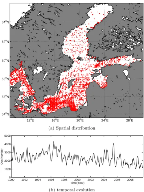
Figure 1: The (a) spatial locations and (b) actual number of records of the T/S profiles assimilated into the model for each month from 1990 to 2009.
1
Fig. 1. The (a) spatial locations and (b) actual number of records
of the T/S profiles assimilated into the model for each month from 1990 to 2009.
years. The data coverage as a function of space and time is presented in Fig. 1. The number of observations is rang-ing from 1200 to 4000 per month. One noticeable feature is that the number of observations per year has significantly de-creased since 1998.
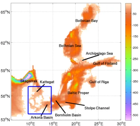
Figure 2: The HBM model domain with depth contours (in m) used for the reanalysis.
2
Fig. 2. The HBM model domain with depth contours (in m) used
for the reanalysis.
The above treatment is crucial for the multi-decadal as-similation experiment. As shown in Fu et al. (2011) and Zhuang et al. (2011), the initial condition with data assim-ilation could reduce the RMSE of the subsequent prediction and the impact generally endures for 2–3 weeks. The per-sistence time scale is larger in the deep bottom layer of the Baltic Sea where the water masses are relatively stationary. Hence, the model state cannot be drastically adjusted dur-ing the assimilation, which will form a spurious cold/warm eddy if there is a large misfit between model and observation. The altered initial state due to one “questionable” measure-ment will cause spikes in the vertical stratification or even instability of the model. This problem can well happen at the beginning of the assimilation experiment because the model differs largely from the observations in the bottom layer. As the model state is gradually rendered close to observations with the continuous insertion of measurement information, the criteria based on innovations will be loosened. In total, there are about 82 354 temperature and 79 148 salinity mea-surements combined into the model. About 2000 observa-tions are withheld for validating the reanalysis as indepen-dent data. With the above quality control, about 8 % temper-ature and 9 % salinity measurements are discarded from the original dataset.
3 Model configuration
3.1 Physical model
The model used in this study is a two-way nested, free sur-face, hydrostatic three-dimensional (3-D) circulation model HIROBM-BOOS (HBM). The model code forms the basis of a common Baltic Sea model for providing GMES Ma-rine Core Service since 2009. The finite difference method is adopted for its spatial discretization in which a staggered Arakawa C grid is applied on a horizontally spherical and vertically z-coordinate. A detailed description of the model can be found in Berg and Poulsen (2011).
In this study, the model is set up with a coarser resolu-tion than the model’s operaresolu-tional set up. It has a 6 nautical mile (nm) horizontal resolution for the Baltic–North Sea. In the Danish Water, a domain with 1 nm resolution is two-way nested with the Baltic Sea (Fig. 2). A high resolution model in the Danish water is very important for multi-decadal sim-ulations because it helps to more realistically reproduce the narrow deep transports between the North Sea and Baltic Sea. The 3-D model for the Baltic–North Sea has in total 50 vertical layers. The top layer thickness is selected at 8 m in the coarse resolution Baltic–North Sea model in order to avoid tidal drying of the first layer in the English Strait. The rest of the layers in the upper 80 m have 2 m vertical resolution. The layer thickness below 80 m increases grad-ually from 4 m to 50 m. In the nested domain, the vertical resolution is increased to 52 levels to resolve the complex bathymetry in the shallow inner Danish waters. The top layer is 2 m thick and then with a 1 m or 2 m layer thickness for the rest of 51 layers.
The meteorological forcing is based on a reanalysis us-ing the regional climate model HIRHAM through a dy-namic downscaling (including a daily re-initialization) from ERA-Interim Global reanalysis. HIRHAM is a regional at-mospheric climate model (RCM) based on a subset of the HIRLAM and ECHAM models, combining the dynam-ics of the former model with the physical parameteriza-tion schemes of the latter. The HIRLAM model – High Resolution Limited Area Model – is a numerical short-range weather forecasting system developed by the in-ternational HIRLAM Programme (http://hirlam.org). The ECHAM global climate model (GCM) is a general atmo-spheric circulation model developed at the Max Planck In-stitute of Meteorology (MPI) in collaboration with external partners. The original HIRHAM model was a collaboration between DMI, the Royal Netherlands Meteorological Insti-tute (KNMI) and MPI. A detailed description of HIRHAM Version 5 can be found in Christensen et al. (2007).
3.2 Experimental setup
Two experiments spanning 1990–2009 have been carried out in this study. The surface momentum and heat fluxes in the
1990 1991 1992 1993 1994 1995 1996 1997 1998 1999 2000 2001 2002 2003 2004 2005 2006 2007 2008 2009 −3
−2 −1 0 1 2
Bias(
°
C)
Model Assim
(a) SST BIAS
1990 1991 1992 1993 1994 1995 1996 1997 1998 1999 2000 2001 2002 2003 2004 2005 2006 2007 2008 20090 0.5
1 1.5 2 2.5 3
RMSE(
°
C)
Model Assim
(b) SST RMSE
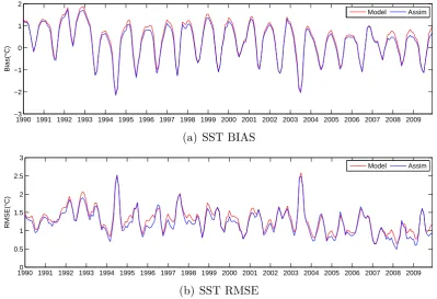
Figure 3: The evolution of basin-averaged (a) bias (b) RMSE calculated
against monthly mean satellite SST from 1990 to 2009.
3
Fig. 3. The evolution of basin-averaged (a) bias and (b) RMSE calculated against monthly mean satellite SST from 1990 to 2009.
model are calculated by using bulk formulations. The ther-modynamics of the ice is built on Semtner’s layer model (Semtner, 1976). Hourly HIRHAM data of 10 m wind, 2 m air temperature, mean sea level pressure, surface humidity and cloud cover was used on the ocean model grid with a horizontal resolution of about 12 km. The surface heat flux was parameterized using bulk quantities of both atmosphere and sea or sea ice and taken into account only in the heat budget calculations. River fresh water discharge data was av-eraged daily based on a combination of measurements and hydrological simulations. The lateral boundary condition in the North Sea contains three components: a tidal sea level derived from 17 major tidal constituents; a surge component derived from a Northeast Atlantic two-dimensional surge model (in 6 nm resolution) and a density profile derived from ICES T/S monthly climatology. Though the model domain covers the whole Baltic–North Sea, the results in the North Sea are not the focus of this paper. Compared to the Baltic Sea, the North Sea has different hydrographic features. This renders it difficult to cover all detailed comparisons and dis-cussions of both seas in a single paper.
The experiment without data assimilation is referred to as the free run. A second experiment is carried out with the same forcing but the ICES T/S profile data was assimilated with the 3DVAR scheme described in Sect. 2.1. Assimilation time window is 1 day, i.e., the assimilation is performed daily provided that any observations are available. During the as-similation, observations for one day are combined into the
initial state of the model at the end of a day and the updated model state will serve as the new initial state. The number of assimilated observations is shown in Fig. 2. The number ranges from 1000 to 4100 for different months, not necessar-ily increasing with time. For both experiments, model output is saved hourly to meet the requirements in applications that need high temporal resolution.
4 Results
To present an overview of the quality of the reanalysis, we validate the monthly mean reanalysis against a variety of ob-servations. The misfit between model and observation is as-sessed with sea level measurements from tide gauge stations, satellite SST and independent in situ observations. The cor-relation coefficients, evolution of RMSE (Root Mean Square Error) and bias, are presented for the period 1990–2009. 4.1 Temperature
4.1.1 SST verification
19900 1992 1994 1996 1998 2000 2002 2004 2006 2008 5
10 15 20
Temperature(
°
C)
(a) 15 m
19900 1992 1994 1996 1998 2000 2002 2004 2006 2008
5 10 15
Temperature(
°
C)
(b) 50 m
19900 1992 1994 1996 1998 2000 2002 2004 2006 2008
5 10 15
Temperature(
°
C)
(c) 80 m
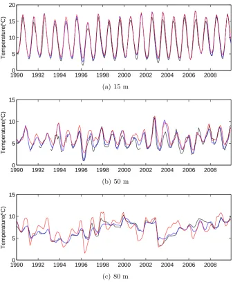
Figure 4: The time series of temperature at (55.15
◦N, 15.92
◦E) for the depth
of (a) 15 m, (b) 50 m and (c) 80 m. The red is the free run, the blue is the
reanalysis and the black is for observations.
4
Fig. 4. The time series of temperature at 55.15◦N, 15.92◦E for the depth of (a) 15 m, (b) 50 m, and (c) 80 m. The red is the free run, the blue
is the reanalysis and the black is for observations.
varying bias of 1–1.5◦C, with the peak in the winter and cold bias in the summer. The RMSE is reduced to 1.69◦C after the assimilation, whereas the bias is only reduced by 0.09◦C. From our previous validations (Høyer and She, 2007), the large seasonal bias in the free run can be largely attributed to the errors in the forcing and/or heat flux parameterization used in the ocean model. This bias cannot be eliminated by the assimilation of only sparse T/S profiles. An interesting feature is that the major SST error reduction due to the assim-ilation occurs in winter when fewer observations are found. 4.1.2 Temperature profile verification using
indepen-dent data
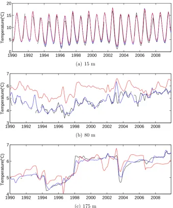
The time series of temperature is compared with independent observations located at 55.15◦N, 15.92◦E in the Bornholm
Basin and at 57.15◦N, 19.92◦E in the Baltic Proper. These two locations were withheld from the assimilation because they have relatively complete records for the period 1990– 2009. In the Bornholm Basin, the upper layer of the sea is subject to strong annual and semi-annual variations. Accord-ing to Fu et al. (2011), the annual and semi-annual cycles account for 70 percent of the total variance in the tempera-ture. From Fig. 4, the characteristics in the observations are well reproduced by the model for the whole period. The tem-perature at 15 m exhibits strong annual and semi-annual vari-ations. The temperature differs by about 10◦C between win-ter and summer, whereas the inwin-ter-annual variability is much weaker. The correlation coefficient between model and ob-servation is very high (0.98) for the 20 year period. By com-parison, temperature in the reanalysis is slightly improved by 0.1–0.3◦C in several months. The depth of 50 m can be
19900 1992 1994 1996 1998 2000 2002 2004 2006 2008 5
10 15 20
Temperature(
°
C)
(a) 15 m
19903 1992 1994 1996 1998 2000 2002 2004 2006 2008
4 5 6 7
Temperature(
°
C)
(b) 80 m
19904 1992 1994 1996 1998 2000 2002 2004 2006 2008
5 6 7
Temperature(
°
C)
(c) 175 m
Figure 5: The time series of temperature at (57.15
◦N, 19.92
◦E) for the depth
of (a) 15 m, (b) 80 m and (c) 175 m. The red is the free run, the blue is the
reanalysis and the black is for observations.
5
Fig. 5. The time series of temperature at 57.15◦N, 19.92◦E for the depth of (a) 15 m, (b) 80 m, and (c) 175 m. The red is the free run, the
blue is the reanalysis and the black is for observations.
a good representation of primary halocline in the Bornholm basin that typically lies at about 40–60 m. At this depth, the temperature in the intermediate water is less subject to an-nual and semi-anan-nual variations than at the surface. Notably, the effect of assimilation is more evident than at the depth of 15 m. The correlation coefficient is increased from 0.74 in the free run to 0.81 in the reanalysis while the mean RMSE is re-duced from 1.27◦C to 0.98◦C. The temperature at the depth
of 80 m may represent the temperature at the bottom layer. It is found that the reanalysis temperature is much closer to the observations than the free run. The misfit substantially drops from 1.20◦C to 0.49◦C while the correlation coeffi-cients increase from 0.72 to 0.91. It suggests that the reanal-ysis reproduces more realistic variations of the temperature near the bottom layer.
In the central Baltic Proper, the water column is perma-nently stratified and the halocline lies at about 60–80 m. The two model run show similar error features as in the Born-holm Basin station. The temperature at 57.15◦N, 19.92◦E is well simulated by the model at the depth of 15 m (Fig. 5a) with a model-data correlation coefficient of 0.96. However, the free run overestimates the temperature at 50 m depth by
∼1◦C (Fig. 5b). As the model’s resolution is inadequate to
1990 1992 1994 1996 1998 2000 2002 2004 2006 2008 −0.5
0 0.5 1 1.5
Bias(
°
C)
Time(Year)
(a) total mean bias
1990 1992 1994 1996 1998 2000 2002 2004 2006 2008 0.5
1 1.5 2 2.5 3
RMSE(
°
C)
Time(Year)
(b) total mean RMSE
1990 1992 1994 1996 1998 2000 2002 2004 2006 2008 −1
0 1 2
Bias(
°
C)
Time(Year)
(c) bias below 60 m
19900 1992 1994 1996 1998 2000 2002 2004 2006 2008 0.5
1 1.5 2 2.5
RMSE(
°
C)
Time(Year)
(d) RMSE below 60 m
Figure 6: The mean RMSE and bias of temperature caculated with monthly
mean data from 1990 to 2009: (a) total mean RMSE, (b) total mean bias,
(c) mean RMSE below 60 m and (d) mean bias below 60 m. The red is the
free run and the blue is the reanalysis.
6
Fig. 6. The mean RMSE and bias of temperature caculated with monthly mean data from 1990 to 2009: (a) total mean bias, (b) total mean
RMSE, (c) mean bias below 60 m, and (d) mean RMSE below 60 m. The red is the free run and the blue is the reanalysis.
of deep layer, which is dominated by inter-annual variabil-ity (Fig. 5c). Changes of the water mass in this area are strongly linked to large-scale atmospheric variability (Stige-brandt and Gustafsson, 2003). For instance, the temperature is 1◦C higher from 1998 onward than the period 1990–1998. Similarly, the reanalysis data fit better with the observations for most of the time. The RMSE is decreased from 0.42◦C to 0.17◦C, whereas the correlation coefficient is noticeably increased from 0.79 to 0.96.
4.1.3 Temperature profile verification using all data
To facilitate the comparison, the observed profiles are binned into 10 km×10 km×1 month bins corresponding to the model grid. In addition, the bias and RMSE are also cal-culated below the permanent halocline depth in the central Baltic where the model tends to have a large bias. The total RMSE and bias of both runs are shown in Fig. 6. In Fig. 6a, the model has clear warm bias in the Baltic Sea. The mean bias is about 0.69◦C for the whole basin and on all seasons. Notably, the seasonal warm bias is not consistent with the SST verification results in Sect. 4.1.1 where a strong cold bias is shown in summer. A possible explanation is that there is a significant warm bias in the model subsurface layer so that the cold bias in summer is compensated by the subsur-face warm bias. In addition, the bias is smaller in winter than in summer for most years, which is consistent with our pre-vious validations. During summer, a very shallow seasonal thermocline develops in the Baltic Sea when the surface cold water is heated. In the shallow western area, there is a change between stratification and well-mixed conditions. At present, modeling the seasonal thermocline is still a challenging prob-lem even for the high resolution coastal models, which tend to result in big errors of the temperature in summer. In the reanalysis, the mean bias is typically less than the free run. For the whole Baltic Sea, it is reduced to 0.37◦C. In partic-ular, the warm bias is significantly reduced from 0.78◦C to 0.20◦C below 60 m (Fig. 6c). This demonstrates the benefit of data assimilation for systematic errors. It should be noted, the comparison is not independent and may be affected by the number of available observations for each month.
Different from the bias, the RMSE of temperature appears to be dominated by seasonal variations in the Baltic Sea, about 2.0◦C in summer and 1.0◦C in winter. As explained above, the model has bias in the summertime, which forms a large portion of the RMSE. By comparison, the RMSE is generally reduced in the reanalysis for the 20 years. For example, the mean RMSE is 1.58◦C for the Baltic Sea for
the free run while it was reduced to 1.37◦C in the reanaly-sis (Fig. 6c). Below 60 m, the RMSE is markedly reduced from 1.38◦C to about 0.89◦C in the reanalysis (Fig. 6d). Mean bias reflects the time-mean component of the system-atic errors due to model deficiencies. Meanwhile, the time-varying components could result from inaccuracies in the time varying boundary forcing. This part is relatively
dif-ficult to be remedied with the current assimilation scheme. For example, the total bias for the Baltic Sea is reduced from 0.69◦C to 0.37◦C while the RMSE is still about 1.37◦C in
the reanalysis. 4.2 Salinity
4.2.1 Salinity profile verification using independent data
1990 1992 1994 1996 1998 2000 2002 2004 2006 2008 6.5
7 7.5 8 8.5
Salinity(PSU)
(a) 15 m
19906 1992 1994 1996 1998 2000 2002 2004 2006 2008
8 10 12 14
Salinity(PSU)
(b) 50 m
19905 1992 1994 1996 1998 2000 2002 2004 2006 2008
10 15 20
Salinity(PSU)
(c) 80 m
Figure 7: The time series of salinity at (55.15
◦N, 15.92
◦E) for the depth of
(a) 15 m, (b) 50m and (c) 80 m. The red is the free run, the blue is the
reanalysis and the black is for observations.
7
Fig. 7. The time series of salinity at 55.15◦N, 15.92◦E for the depth of (a) 15 m, (b) 50 m, and (c) 80 m. The red is the free run, the blue is
the reanalysis and the black is for observations.
the salinity in the reanalysis is much closer to the observa-tions at 80 m than the free run. The correlation coefficient with the observations is about 0.68 and 0.74 for the free run and reanalysis, respectively.
The time series of salinity at Gotland Deep station (57.15◦N, 19.92◦E) is shown in Fig. 8 for the upper, in-termediate and bottom layer. At 15 m depth, salinity of the free run is typically improved by the assimilation (Fig. 8a). The mean RMSE is considerably decreased from 0.31 psu to 0.13 psu while the correlation coefficient is increased from 0.49 to 0.78. In addition, the decreasing tendency in the salin-ity of the free run is absent from the reanalysis and observa-tion. At the depth of 80 m (Fig. 8b), the salinity is slightly in-creased from 1990 to 2009 in the observations, which could be associated with the saline water intrusion. However, the
increasing trend is absent in the free run. In the reanaly-sis, the variations of salinity is much more consistent with the observations than the free run as the correlation coeffi-cient is significantly increased from 0.18 to 0.62. Further, the RMSE is reduced from 0.86 psu to 0.38 psu. Water be-low the primary halocline of the Baltic Proper is compar-atively steady and its natural variation is strongly related to the large-scale atmospheric variability and the accumu-lated freshwater inflow (Stigebrandt and Gustafsson, 2003; Meier and Kauker, 2003). This can be demonstrated from the salinity at the depth of 175 m (Fig. 8c). The observa-tions show a pronounced increasing trend from 1990 to 2009. The salinity reaches 12.5 psu from 2004 to 2009, indicating strong saline water intrusion. Without the assimilation, bot-tom saline water in the free run is gradually diluted due to
1990 1992 1994 1996 1998 2000 2002 2004 2006 2008 5.5
6 6.5 7 7.5
Salinity(PSU)
(a) 15 m
19907 1992 1994 1996 1998 2000 2002 2004 2006 2008
8 9 10 11
Salinity(PSU)
(b) 80 m
19909 1992 1994 1996 1998 2000 2002 2004 2006 2008
10 11 12 13
Salinity(PSU)
(c) 175 m
Figure 8: The time series of salinity at (57.15
◦N, 19.92
◦E) for the depth of (a)
15 m, (b) 80 m and (c) 175 m. The red is the free run, the blue is reanalysis
and the black is for observations.
8
Fig. 8. The time series of salinity at 57.15◦N, 19.92◦E for the depth of (a) 15 m, (b) 80 m, and (c) 175 m. The red is the free run, the blue is
reanalysis and the black is for observations.
the strong vertical mixing of the model, which also affects the simulation of inflow events. The salinity is about 2 psu lower than the observations. The effect of the assimilation could be sustained for a long time because of the steady ter masses in this region. Once the state of the bottom wa-ter is changed, it won’t be fully replaced until another ma-jor inflow intrudes. The reanalysis presents remarkable im-provements as the salinity is generally increased by 2 psu. In addition, the major inflow events are more consistent with the observations except in 2006–2008. The RMSE is reduced from 2.31 psu to 0.27 psu while the correlation coefficient is increased from 0.78 to 0.89.
4.2.2 Salinity profile verification using all data
1990 1992 1994 1996 1998 2000 2002 2004 2006 2008 −1
−0.5 0 0.5
Bias(PSU)
Time(Year)
(a) total mean bias
1990 1992 1994 1996 1998 2000 2002 2004 2006 2008 0.5
1 1.5 2 2.5
Time(Year)
RMSE(PSU)
(b) total mean RMSE
1990 1992 1994 1996 1998 2000 2002 2004 2006 2008 −3
−2 −1 0 1
Bias(PSU)
Time(Year)
(c) mean bias below 60 m
19900 1992 1994 1996 1998 2000 2002 2004 2006 2008 1
2 3 4
Time(Year)
RMSE(PSU)
(d) mean RMSE below 60 m
Figure 9: The mean RMSE and bias of salinity caculated with monthly mean
data from 1990 to 2009: (a) total mean RMSE, (b) total mean bias, (c) mean
RMSE below 60 m and (d) mean bias below 60 m. The red is the free run
and the blue is the reanalysis.
9
Fig. 9. The mean RMSE and bias of salinity calculated with monthly mean data from 1990 to 2009: (a) total mean bias, (b) total mean
RMSE, (c) mean bias below 60 m, and (d) mean RMSE below 60 m. The red is the free run and the blue is the reanalysis.
1990 1992 1994 1996 1998 2000 2002 2004 2006 2008 −0.2
0 0.2 0.4 0.6
Sea level(m)
Time(Year)
Obs Assim Model
(a) Gadser
1990 1992 1994 1996 1998 2000 2002 2004 2006 2008 −0.4
−0.2 0 0.2 0.4 0.6
Sea level(m)
Time(Year)
Obs Assim Model
(b) Hornbaek
1990 1992 1994 1996 1998 2000 2002 2004 2006 2008 −0.4
−0.2 0 0.2 0.4 0.6
Sea level(m)
Time(Year)
Assim Model Obs
(c) Diff between Gadser and Hornbaek
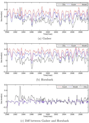
Figure 10: The time series of sea level at Gedser (55.15
◦N, 15.92
◦E),
Horn-baek (55.15
◦N, 15.92
◦E)) and (c) the difference between (a) and (b).The red
is the free run, the blue is the reanalysis and the black is for observations.
10
Fig. 10. The time series of sea level at Gedser (55.15◦N, 15.92◦E), Hornbæk (55.15◦N, 15.92◦E), and (c) the difference between (a) and
(b). The red is the free run, the blue is the reanalysis and the black is for observations.
the mean RMSE is 1.46 psu for the Baltic Sea in the free run (Fig. 9b), while it is reduced to 1.15 psu in the reanalysis. Below 60 m, the RMSE is largely reduced from 1.74 psu to about 0.83 psu in the reanalysis due to the improvement on the simulation of inflow (Fig. 9d).
4.3 Sea level
Since sea level is a very good indicator of the model behav-ior with respect to the barotropic dynamics of the system, it is one of the most important variables to be assessed in the
Table 1. The correlation coefficients, bias (in m) and RMSD (in m) of the model compared to observed tide gauge data in 14 stations. The
RMSD is calculated with the residual of time series after the mean is subtracted.
Position (degrees) Reanalysis Free run
Corr. coeff. RMSD Bias Corr. coeff. RMSD Bias
Aarhus 56.15◦N, 10.22◦E 0.785 0.0668 0.1044 0.7453 0.0692 0.2069
Frederikshavn 57.43◦N, 10.57◦E 0.827 0.0641 0.1569 0.8033 0.0661 0.2621
Slipshavn 55.28◦N, 10.83◦E 0.783 0.0605 0.1084 0.7501 0.0611 0.2100
Korsor 55.33◦N, 11.13◦E 0.7255 0.0691 0.0922 0.7124 0.0667 0.1934
Hornbæk 56.10◦N, 12.47◦E 0.8776 0.0581 0.1712 0.8588 0.0608 0.2728
Rodby 54.65◦N, 11.35◦E 0.5268 0.1014 0.0644 0.5367 0.0989 0.1655
Gedser 54.57◦N, 11.93◦E 0.6794 0.0869 0.1035 0.6766 0.0854 0.2045
Tejn 55.25◦N, 14.83◦E 0.8775 0.0656 0.2353 0.8756 0.0649 0.3349
Kalix 65.68◦N, 23.13◦E 0.9153 0.0858 0.3847 0.9159 0.0856 0.4916
Klagshamn 55.52◦N, 12.75◦E 0.8626 0.0578 0.2231 0.8358 0.0618 0.3241
Kungsholmsfort 56.08◦N, 15.54◦E 0.9001 0.0609 0.2700 0.8844 0.0644 0.3716
Kungsvik 58.78◦N, 11.13◦E 0.9008 0.0526 0.1594 0.8848 0.0564 0.2646
Ratan 63.98◦N, 20.88◦E 0.9496 0.0622 0.3771 0.9480 0.0636 0.4835
Visby 57.63◦N, 18.28◦E 0.9378 0.0540 0.2970 0.9318 0.0559 0.3971
Since no sea level data are assimilated, the comparison is completely independent.
From Table 1, most of the stations are located in the tran-sition zone between the North Sea and the Baltic Sea. In this transition zone, a general estuarine circulation forms a regional scale frontal system from northern Kattegat to the Arkona Sea. Numerical modeling in this region re-quires high-resolution bathymetry usually achieved by nest-ing model system (She et al., 2007). Compared with tide gauge, the correlation coefficients at 9 stations are all larger than 0.8. At Rodby and Gedser, the coefficients are 0.52 and 0.67, respectively. These two stations are located near the Darss Sill where the sub-grid scale feature of narrow trans-port cannot be fully resolved even in a high resolution nested model. In general, it is encouraging that the reanalysis is bet-ter correlated with the tide gauge data than the free run by 2–5 %. In addition, the mean bias of sea level is substantially reduced by about 0.1 m for all stations, indicating the im-pact of T/S assimilation. In fact, assimilation of temperature is equivalent to modifying thermal expansion while assimi-lation of salinity amounts to altering water volume. The in-duced variations in the density will cause regional changes in sea level. However, we find that the redistributed density field mainly contributed to reducing the mean bias of the model. In Table 1, the RMSD is also calculated similarly as the RMSE by using the residual of time series whose mean is subtracted. The reduction of RMSD could reflect the impact of assimila-tion on the time-varying component of the systematic errors. From Table 1, the changes in RMSD are less than 1 cm for most stations. It suggests that the assimilation of sparse T/S profiles behaves more effectively in rectifying the time-mean component of systematic errors.
The transition zone between the North Sea and the Baltic Sea is characterized by a brackish Baltic Sea outflowing in
the upper layer and a saline North Sea inflow in the bottom layer. Time series of sea level at Gedser and Hornbæk are presented in Fig. 10. In the free run, sea level is generally higher than the tide gauge data. Sea level in the reanalysis is decreased after the assimilation and closer to observations. As shown in Table 1, the improvements are essentially due to the reduction of the mean bias. Sea level differences be-tween Hornbæk and Gedser can be regarded as a barotropic transport index. The barotropic transport through the area is relatively large, with instantaneous transport that can be an order of magnitude larger than the annually averaged estu-arine flow (Bendtsen et al., 2009). This transport is forced by the water level difference between the northern Kattegat and the Arkona Sea. From Fig. 10c, the water level difference between Hornbæk and Gedser shows very minor changes be-tween the free run and reanalysis. The strong transport in 1993 is not captured in both experiments. The variations in the transport are well produced but the magnitude is under-estimated. The assimilation of T/S seems not effective to im-prove the barotropic transport. This is because the density changes of water masses, which are induced by the T/S as-similation, act primarily on the baroclinic transport through the Danish transition zone.
4.4 Mixed layer depth (MLD)
Mixed layer depth is an important variable for determining seasonal climate signals, and primary biogeochemical fea-tures in marine ecosystems. With very deep mixed layers, the phytoplankton are unable to get enough light to main-tain their metabolism. The shallowing of the mixed layers during spring in the North Atlantic is therefore associated with a strong spring bloom of plankton. The mixed layer is characterized by being nearly uniform in properties such as
12o
E 16o
E 20oE 24o
E 28oE
54o N 56o N 58o N 60o N 62o N 64o N
(a) MLD without ASSIM in January
12o
E 16o
E 20oE 24o
E 28oE
54o N 56o N 58o N 60o N 62o N 64o N 0 5 10 15 20 25 30 35 40 45 50 55 60
(b) MLD with ASSIM in January
12o
E 16o
E 20oE 24oE 28oE
54o N 56o N 58o N 60o N 62o N 64o N
(c) MLD without ASSIM in July
12o
E 16oE
20oE 24oE 28oE
54o N 56o N 58o N 60o N 62o N 64o N 0 3 6 9 12 15 18
(d) MLD with ASSIM in July
12o
E 16o
E 20oE 24oE 28oE
54o N 56o N 58o N 60o N 62o N 64o N −10 −5 0 5 10 15 20
(e) MLD difference in January
12o
E 16o
E 20oE 24oE 28oE
54o N 56o N 58o N 60o N 62o N 64o N −2 −1.5 −1 −0.5 0 0.5 1 1.5 2
(f) MLD difference in July
Figure 11: The climatological mean mixing layer depth (MLD) calculated from the free run and reanalysis for 20-year period.
11
Fig. 11. The climatological mean mixed layer depth (MLD) (unit: m) calculated from the free run and reanalysis for 20-year period.
temperature and salinity throughout the layer. The depth of the mixed layer is often determined by hydrographic mea-surements of water properties. Two criteria often used to de-termine the mixed layer depth are temperature and sigma-t (density) changes from a reference value. In this study, the temperature criterion as used in Levitus (1982) is chosen to define the mixed layer as the depth at which the temperature change from the surface value exceeds 0.5◦C.
The climatological mixed layer depths from both experi-ments are presented in Fig. 11 for winter (January) and sum-mer (July). In the Baltic Sea, the primary force for driving
in late winter. Therefore, the mean mixed layer depth dif-fers by 20 m between winter and summer. Particularly in the Baltic Proper, the mixed layer depth is only about 10 m in summer but is considerably deepened to 40–60 m in win-ter (Fig. 11b). The wawin-ter column of this area in winwin-ter is well mixed and vertically homogeneous down to the halo-cline (about 60–70 m in central Baltic Sea).
Why do larger changes occur in the MLD of winter after the assimilation than the summer? If the free run does not produce the adequately accurate MLD in summer, it must be that the controlling effect of meteorological forcing is too strong to alter via the assimilation. Forcing itself is unlikely the main cause as the reanalysis winds are quite accurate. In summer, the mixed layer is strongly linked to the surface Ek-man flow. The modeled upper layer thus depends primarily upon the accuracy of the meteorological forcing used to force the system. The surface forcing could quickly dissipate the changes of temperature and salinity caused by the data assim-ilation. Another important reason is the gradually increasing heating effect, which contributes to the formation of a sea-sonal thermocline at about 10–20 m depth from spring. In summer, the heating is strongest and plays a dominant role in the formation of the mixed layer. The mixed layer is largely confined to several meters near the surface above the ther-mocline. In this case, mixed layer may not benefit substan-tially from the assimilation when the role of meteorological forcing is dominant. The effect of assimilation is also weak in shallow coastal waters such as the Danish transition zone because the entire water column can be a turbulent bound-ary layer through the year. For instance, deep mixed layer in summer mainly occur near the coast, like the southern coast of the central Baltic Sea, in southern Skagerrak and in the Archipelago Sea.
Evolution of the MLD at 57.15◦N, 19.92◦E and mean simulated MLD for the Baltic Sea are presented in Fig. 12. As explained above, the MLD displays a clear seasonal cycle and is typically larger in winter than in summer for the mean value in the Baltic or at the given location. Both the free run and the reanalysis MLD at 57.15◦N, 19.92◦E are in good agreement with the observations in summer, which helps to substantiate the results from the reanalysis in Fig. 11f. The most significant differences between the free run and the re-analysis occur in wintertime, which is also consistent with Fig. 11e. In this sense, Fig. 11e indeed shows an improve-ment on the MLD in the free run after the T/S assimilation. It is noted that even after assimilation, the model MLD in winter is still shallower than observations.
5 Conclusions and discussions
In this paper, a 3DVAR scheme is used to construct a ret-rospective analysis of temperature, salinity, and sea level in the Baltic Sea from 1990 to 2009. The goal of this reanaly-sis is two-fold: first, the performance of the 3DVAR scheme
can be assessed in a multi-decadal integration and provide more experience for future operational applications; second, the reanalysis can provide a uniformly gridded dataset for studies such as model intercomparisons, physical processes, climate variability and other purposes in the Baltic Sea. The accuracy of the reanalysis is quantified by direct comparisons against independent sea level, temperature and salinity mea-surements. Particular attention is focused on the effect of as-similation on reducing the bias and RMSE of model forecast. We begin with a comparison with time series of temper-ature and salinity that has relatively complete records in the Bornholm Basin and Baltic Proper. For these two locations, time series of temperature and salinity are generally im-proved in the reanalysis and fit better with the observations than the free run. The RMSE of temperature and salinity is substantially reduced for different depths while the correla-tion coefficients between model and observacorrela-tion are largely increased. In particular, the salinity related to the saline wa-ter intrusion in this region is markedly improved in the re-analysis. Major inflow events such as in 1993 and 2003 are captured more accurately in the reanalysis and the salinity in the bottom layer is increased by 2–3 psu. Statistically, the mean bias of temperature is reduced from 0.69 to 0.37◦C for the whole Baltic Sea while the mean bias of salinity is reduced from−0.52 psu by about−0.18 psu. Similarly, the mean RMSE is generally reduced in the reanalysis by 0.25◦C and 0.3 psu, respectively. In the central Baltic region, the errors associated with the simulation of saline water intru-sion are significantly reduced in the reanalysis with the mean RMSE and bias of salinity reduced by 0.86 psu and 0.91 psu. The reanalysis is further validated against sea level data at 14 tide gauge stations. By comparison, the reanalysis is better correlated with the measurements than the free run as the correlation coefficients are increased by 2 %–5 % for most stations. In addition, the RMSE is generally reduced by 10 cm in the reanalysis. The reduction of RMSE is found to stem mainly from the reduction of mean bias, which is about 10 cm smaller than in the free run. After the mean is subtracted from the time series of sea level, the root mean square difference (RMSD) is also shown to be slightly re-duced (within 1 cm). It suggests that the assimilation of T/S profiles contributes mainly to reducing the time-mean com-ponent of systematic errors of the model. The reduction of the mean bias contributes little to improve the barotropic transport, which is maintained by the water level difference between the northern Kattegat and the Arkona Sea. Differ-ences of sea level between Gedser and Hornbæk are used as a barotropic transport index. It appears that the assimilation acts to raise the whole water column in the Danish waters other than adjust the difference of sea level. Assimilation of T/S profiles plays a more important role in deep waters be-cause changes in density field would redistribute the water mass and adjust the baroclinic transport.
The mean mixed layer depth is compared between the re-analysis and free run for the 20 year period. In the Baltic Sea,
19900 1992 1994 1996 1998 2000 2002 2004 2006 2008 20
40 60 80
MLD(m)
Model Assim Obs
(a) MLD at (57.15◦N 19.92◦E)
19900 1992 1994 1996 1998 2000 2002 2004 2006 2008 10
20 30 40
Time(year)
MLD(m)
Model Assim
(b) mean MLD
Figure 12: The evolution of mixing layer depth (MLD) calculated from the
free run and reanalysis.
12
Fig. 12. The evolution of mixed layer depth (MLD) calculated from the free run and reanalysis.
the mixed layer is important for marine environment and fish-ery as its depth determines the average level of light seen by marine organisms. It is found that the mixed layer depth is typically larger in winter than in summer, differing by 20 m on average. In addition, changes in the mixed layer depth due to the assimilation appear to be minor in summertime and shallow waters. The effect of heating in summer and domi-nant surface forcing could be related to the relatively small effect of the assimilation. In deep waters, however, the ef-fect of the assimilation is significant in wintertime. In the Baltic Proper and Bothnian Sea the mixed layer is deepened by 20 m in the reanalysis. In the Danish transition zone to the Bornholm Basin, the mixed layer depth has small variations throughout the year because the whole water column can be regarded as a turbulent boundary layer.
The results of the reanalysis are encouraging and the as-similation helps to ameliorate some model deficiencies such as the simulation of saline water intrusion into the Baltic Proper. The reanalysis can be regarded as good surrogate data for process studies in the Baltic Sea. Furthermore, the long-term reanalysis helps to identify problems in the as-similation. For instance, the assimilation is less effective in shallow water such as the Danish transition water where the barotropic transport is barely improved. The reduction of RMSE is largely due to the reduction in the model’s mean
bias. The random error is only slightly reduced according to the correlation coefficients. Finally, this reanalysis may be further improved by assimilating more surface observations in addition to T/S profiles. But for this reanalysis, surface observations such as SST and SSH can easily be used for independent comparisons.
implementing a new ice model into the HBM. Furthermore, satellite data play a complementary role to the subsurface in situ observations and will be assimilated into the model in the future.
Acknowledgements. This paper is supported by the EU FP6
MyOcean project (Contract No. 218812). We wish to thank the anonymous reviewers for their useful suggestions. Mathias Bjerre helps to further process the ICES data. We are also grateful to Jacob Woge Nielsen for his useful comments. The help and sug-gestions from other colleagues in the COI/DMI are also appreciated.
Edited by: M. Meier
References
Bendtsen, J., Gustafsson K. E., S¨oderkvist, J., and Hansen, J. L. S.: Ventilation of bottom water in the North Sea-Baltic Sea transition zone, J. Marine Syst., 75, 138–149, 2009.
Bengtsson, L., Hagermann, S., and Hodges, K. I.: Can climate trends be calculated from reanalysis data?, J. Geophys. Res., 109, D11111, doi:10.1029/2004JD004536, 2004.
Berg, P. and Poulsen, J. W.: Implementation details for HBM, DMI Technical Report No. 12-11, ISSN: 1399-1388, Copenhagen, 2011.
Byrd, R. H., Lu, P., Nocedal, J., and Zhu, C.: A limited memory algorithm for bound constrained optimization, SIAM Journal on Scientific Computing, 16, 1190–1208, 1995.
Carton, J. A. and Giese, B. S.: A reanalysis of ocean climate using Simple Ocean Data Assimilation (SODA), Mon. Weather Rev., 136, 2999–3017, 2008.
Carton, J. A., Giese, B. S., and Grodsky, S. A.: Sea level rise and the warming of the oceans in the Simple Ocean Data Assimila-tion (SODA) ocean reanalysis, J. Geophys. Res., 110, C09006, doi:10.1029/2004JC002817, 2005.
Christensen, O. B., Drews, M., Christensen, J. H., Dethloff, K., Ke-telsen, K., Hebestadt, I., and Rinke, A.: The HIRHAM Regional
Climate Model Version 5 (β), DMI Tech. Rep. 06-17, pp. 22,
2006.
Christensen, J. H., Carter, T. R., and Rummukainen, M.: Evaluat-ing the performance and utility of regional climate models: the PRUDENCE project, Clim. Change, 81, 1–6, 2007.
Courtier, P., Th´epaut, J. N., and Hollingsworth, A.: A strategy for operational implementation of 4D-Var, using an incremental ap-proach, Q. J. Roy. Meteorol. Soc., 120, 1367–1387, 1994. Dobricic, S. and Pinardi, N.: An oceanographic three-dimensional
variational data assimilation scheme, Ocean Modell., 22, 89– 105, 2008.
Friedrichs, M. A. M., Hood, R., and Wiggert, J.: Ecosystem model complexity versus physical forcing: Quantifi cation of their rela-tive impact with assimilated Arabian Sea data, Deep-Sea Res. II, 53, 576–600, 2006.
Fu, W., Zhu, J., Yan, C., and Liu, H.: Toward a global ocean data as-similation system based on ensemble optimum interpolation: al-timetry data assimilation experiment, Ocean Dynamics, 59, 587– 602, 2009.
Fu, W., Høyer, J. L., and She, J.: Assessment of the three dimen-sional temperature and salinity observational networks in the Baltic Sea and North Sea, Ocean Sci., 7, 75–90, doi:10.5194/os-7-75-2011, 2011.
Grasshoff, K.: The hydrochemistry of landlocked basins and fjords, in: Chemical Oceanography (2nd ed.), edited by: Riley, J. P. and Skirrow, G., Chemical Oceanography, 2, 455–597, 1975. Høyer, J. L. and She, J.: Optimal interpolation of SST for the North
Sea and Baltic Sea systems, J. Marine Syst., 65, 176–189, 2007. Jakobsen, F.: The major inflow to the Baltic Sea during January
1993, J. Mar. Syst., 6, 227–240, 1995.
Kishi, M. J., Kashiwai, M., Ware, D. M., Megrey, B. A., Es-linger, D. L., Werner, F. E., Aita, M. N., Azumaya, T., Fujii, M., Hashimoto, S., Huang, D., Iizumi, H., Ishida, Y., Kang, S., Kan-takov, G. A., Kim, H.-C. Komatsu,, K., Navrotsky, V. V., Smith, S. L., Tadokoro, K., Tsuda, A., Yamamura, O., Yamanaka, Y., Yokouchi, K., Yoshie, N., Zhang, J., Zuenko, Y. I., and Zvalin-sky, V. I.: NEMURO a lower trophic level model for the North Pacific marine ecosystem, Ecol. Model., 202, 12–25, 2007. Larsen, J., Høyer, J. L., and She, J.: Validation of a hybrid optimal
interpolation and Kalman filter scheme for sea surface tempera-ture assimilation, J. Marine Syst., 65, 122–133, 2007.
Lepp¨aranta, M. and Myrberg, K.: Physical oceanography of the Baltic Sea. Springer-Verlag, Berlin, 2009.
Levitus, S.: Climatological Atlas of the World Ocean, NOAA Pro-fessional Paper 13, US Department of Commerce, 1982. Liu, Y., Zhu, J., She, J., Zhuang, S., and Gao, J.:
Im-pacts of assimilating ocean profile observations using a bottom-topography-following recursive filter on ocean fore-casting in North Sea/Baltic Sea, Ocean Modell., 26, 75–87, doi:10.1016/j.ocemod.2009.06.005, 2009.
Lorenc, A. C.: Development of an operational variational assimila-tion scheme, J. Meteorol. Soc. Japan, 75, 339–346, 1997. Meier, H. E. M. and Kauker, F.: Modeling decadal variability of the
Baltic Sea. Part 2: The role of freshwater inflow and large-scale atmospheric circulation for salinity, J. Geophys. Res., 108, C11, doi:10 1029/2003JC001799, 2003.
Pemberton, P.: Validation of a one year simulation of the Baltic Sea with optimized boundary conditions, improved bathymetry and data assimilation, European Operational Oceanography: Present and Future, EuroGOOS Office, Sweden, and European Commis-sion, Belgium, pp. 526–530, 2006.
Semtner Jr., A. J.: A model for the thermodynamic growth of sea ice in numerical investigations of climate, J. Phys. Oceanogr., 6, 379–389, 1976.
She, J., Berg, P., and Berg, J.: Bathymetry impacts on water ex-change modelling through the Danish Straits, J. Marine Syst., 65, 450–459, 2007.
Stigebrandt, A. and Gustafsson, B. G.: Response of Baltic Sea to climate change – Theory and observations, J. Sea Res., 49, 243– 256, 2003.
Zhuang, S. Y., Fu, W. W., and She, J.: A pre-operational three Dimensional variational data assimilation system in the North/Baltic Sea, Ocean Sci., 7, 771–781, doi:10.5194/os-7-771-2011, 2011.