© Author(s) 2010. This work is distributed under the Creative Commons Attribution 3.0 License.
of the Past
A unified proxy for ENSO and PDO variability since 1650
S. McGregor, A. Timmermann, and O. Timm
IPRC, SOEST, University of Hawaii at Manoa, Hawaii, USA
Received: 24 August 2009 – Published in Clim. Past Discuss.: 23 September 2009 Revised: 1 December 2009 – Accepted: 6 December 2009 – Published: 5 January 2010
Abstract. In this manuscript we have attempted to
consol-idate the common signal in previously defined proxy recon-structions of the El Ni˜no-Southern Oscillation into one indi-vidual proxy titled the Unified ENSO Proxy (UEP). While correlating well with the majority of input reconstructions, the UEP provides better representation of observed indices of ENSO, discrete ENSO events and documented historical chronologies of ENSO than any of these input ENSO recon-structions. Further to this, the UEP also provides a means to reconstruct the PDO/IPO multi-decadal variability of the Pacific Ocean as the low-pass filtered UEP displays multi-decadal variability that is consistent with the 20th century variability of the PDO and IPO. The UEP is then used to describe changes in ENSO variability which have occurred since 1650 focusing on changes in ENSOs variance, multi-year ENSO events, PDO-like multi-decadal variability and the effects of volcanic and solar forcing on ENSO. We find that multi-year El Ni˜no events similar to the 1990–1995 event have occurred several times over the last 3 1/2 centuries. Consistent with earlier studies we find that volcanic forcing can induce a statistically significant change in the mean state of ENSO in the year of the eruption and a doubling of the probability of an El Ni˜no (La Ni˜na) event occurring in the year of (three years after) the eruption.
1 Introduction
The El Ni˜no-Southern Oscillation (ENSO) is a coupled tropi-cal Pacific ocean-atmosphere phenomenon which is the most dominant global source of interannual climate variability. ENSO is an oscillation characterized by marked changes in eastern equatorial Pacific sea surface temperature (SST),
Correspondence to: S. McGregor ([email protected])
known as El Ni˜no, and a related large scale seesaw in atmo-spheric sea level pressure between the Australia-Indonesian region and the south-central tropical Pacific known as the Southern Oscillation. ENSO influences extreme weather events such as drought, flooding, bushfires and tropical cy-clone activity across vast regions of the globe (Chan, 1985; Nicholls, 1985; Power et al., 1999). While the importance of its climatic impacts are relatively well known, many charac-teristics of the long term changes in ENSO frequency, magni-tude and duration remain unknown. Further to this, whether ENSO variability has changed due to the already observed anthropogenically-induced climate change and how future projected changes will further influence ENSO are largely unresolved questions (Federov and Philander, 2000; van Old-enborgh et al., 2005; Merryfield, 2006).
For example, over the last few decades ENSO variabil-ity has appeared to shift toward a more El Ni˜no-like state (Federov and Philander, 2000) where the 1980s and 1990s contained the two largest observed El Ni˜no events on record along with a prolonged El Ni˜no-like warming in the trop-ical Pacific Ocean that persisted for approximately 5-yrs in the early 1990s. Many studies have tried to ascertain the cause of these unusual events focusing on the roles of anthropogenically-induced climate change and natural decadal or ENSO variability (Latif et al., 1997; Power and Smith, 2007). At this stage it can not be ruled out with confi-dence that the recent changes of ENSO variability are a man-ifestation of natural variability (Timmermann, 1999).
1650 1700 1750 1800 1850 1900 1950 −3
−2 −1 0 1 2 3
Normalised ENSO reconstructions
Year
a)
16500 1700 1750 1800 1850 1900 1950
1 2
Std deviation
Year
b)
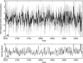
Fig. 1. Time series of (a) the 10 reconstructions (Table 1) of ENSO variability (gray) and the mean of these reconstructions (black). (b) Standard deviation of the 10 reconstructions.
coral records stand as the only way to assess the long term variability of ENSO.
There are currently numerous well crafted reconstructions of ENSO variability which all use a variety of current and paleo proxy data sources and a variety of methods to derive the indices (see discussion in Sect. 2) (Dunbar et al., 1994; Stahle et al., 1998; Cook, 2000; Mann et al., 2000; Evans et al., 2001, 2002; Cobb et al., 2003; Cook et al., 2008; Bra-ganza et al., 2009). Each of these individual reconstructions correlates reasonably well with observations of ENSO vari-ations during the instrumental period. However, while all represent the same signal there is a great deal of variability amongst the proxies (Fig. 1) which acts to reduce confidence in the individual proxies. For example, when looking at the normalized time series of 10 commonly used ENSO proxies (Dunbar et al., 1994; Stahle et al., 1998; Cook, 2000; Mann et al., 2000; Evans et al., 2001, 2002; Cobb et al., 2003; Cook et al., 2008; Braganza et al., 2009), we find that the standard deviation between the proxies at each time step is almost as large as the standard deviation of each index (Fig. 1). This variability amongst the proxy ENSO signals could represent an un-ENSO related climatic signal, an underlying biologi-cal signal, inaccurate proxy dating, or even ENSO itself. Ev-ery ENSO event is different and each event creates a slightly different spatial teleconnection pattern (Trenberth and Stepa-niak, 2001). Therefore proxies derived from different regions could be expected to have slightly different signals of ENSO variability.
Here we attempt to consolidate the information contained in these 10 ENSO reconstructions to come up with a unified ENSO proxy (UEP) that captures the joint features of these reconstructions. This paper is organized as follows. Sect. 2 provides a description of the ENSO proxies used to derive the UEP in this study. Section 3 details the methods used to derive the UEP, while in section 4 the new ENSO proxy is validated against observations and historical documentary chronologies of ENSO. In section 5 we then discuss the vari-ability of ENSO since 1650 and try to put into context the variability of the 20th century. A discussion and conclusions from the study are then presented in Sect. 6.
2 ENSO proxy data
Fig. 2. The location and type of source proxy used in 9 of the 10 original ENSO proxies. See Table 1 for identification the proxy reconstruc-tion corresponding to the proxy number displayed here.
Each of these ENSO proxies uses a variety of input data sources and methods to derive their representation of past ENSO variability. For example, when considering the proxy records used as inputs for these 10 proxies, at one end of the spectrum we have the proxy records of Dunbar et al. (1994) and Cobb et al. (2003) which both source data from corals based in a single region which is directly influenced by ENSO. Whereas, at the other end of the spectrum we have studies like that of Mann et al. (2000) who use a multi-proxy network of diverse multi-proxy indicators located in tropical-subtropical regions that are influenced directly by ENSO or through its teleconnections. It is just as diverse when consid-ering the methods used to derive these proxies from the orig-inal input proxy network. For example, the studies which only include data from one specific source region gener-ally just splice each of the individual records together (Cobb et al., 2003). Whilst studies that use a multi-proxy network generally use a mathematical analysis technique (such as a Principal Component Analysis) to either, identify the com-mon signal within the input proxy network (Braganza et al., 2009), or to decompose the observed data into their dominant spatiotemporal eigenmodes (Mann et al., 2000; Evans et al., 2002). In the latter case, the proxy data are then regressed against the associated times series of the leading eigenmodes during an overlapping period. In such way the regressed proxy data time series and the associated eigenvectors pro-vide an estimate the spatiotemporal variability prior to the observational period.
The data redundancy across the 10 input networks used for the generation of these proxies is relatively small. For instance, there were 155 proxies used in total in the 9 of the 10 input networks and of these, less than 1/4 were used in
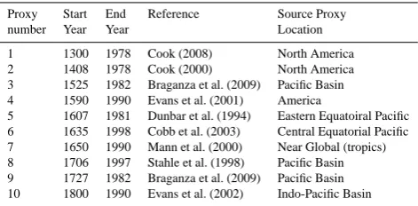
Table 1. ENSO proxies employed in this work.
Proxy Start End Reference Source Proxy
number Year Year Location
1 1300 1978 Cook (2008) North America 2 1408 1978 Cook (2000) North America 3 1525 1982 Braganza et al. (2009) Pacific Basin 4 1590 1990 Evans et al. (2001) America
5 1607 1981 Dunbar et al. (1994) Eastern Equatoiral Pacific 6 1635 1998 Cobb et al. (2003) Central Equatorial Pacific 7 1650 1990 Mann et al. (2000) Near Global (tropics) 8 1706 1997 Stahle et al. (1998) Pacific Basin 9 1727 1982 Braganza et al. (2009) Pacific Basin 10 1800 1990 Evans et al. (2002) Indo-Pacific Basin
1650 1700 1750 1800 1850 1900 1950 −3
−2 −1 0 1 2 3
Proxy ENSO index
Year
Fig. 3. The unified ENSO proxy (UEP) for the period 1650–1978.
Table 2. % variance explained by the first four principal compo-nents along with the normalized eigenvectors for each proxy.
Proxy PC1 PC2 PC3 PC4
Variance 52.5% 13.9% 9.7% 7.1%
Proxy 1 12.3% 9.0% 7.6% 14.5%
Proxy 2 12.3% 7.1% 4.1% 17.5%
Proxy 3 12.4% 10.5% 2.9% 8.2%
Proxy 4 10.1% 3.2% 2.1% 21.9%
Proxy 5 0.0% 14.0% 46.4% 2.6%
Proxy 6 7.5% 25.5% 12.0% 2.3%
Proxy 7 11.3% 3.4% 7.8% 5.7%
Proxy 8 12.9% 1.8% 1.7% 8.5%
Proxy 9 13.1% 4.4% 2.9% 11.6%
Proxy 10 7.8% 21.0% 12.3% 7.0%
American tree ring data in their ENSO reconstruction deriva-tion. This may result in a common mode that is more highly weighted to this ENSO teleconnection region.
3 Methods
The various forms of analysis used to generate ENSO prox-ies from the original multi-proxy network were carried out to isolate the ENSO variability within the network by re-moving the effects of climatic noise (i.e., local climatic and other large scale variability uncorrelated to ENSO) and non-climatic factors (i.e., biological processes). However, due to the large variability between these indices we believe that each of the proxies utilized incorporates, to varying degrees, a noise component that is not related to ENSO (cf. Fig. 1b). Thus, to decompose this new multi-variable ENSO proxy network into a single leading mode of covariability, we carry out a Principal Component Analysis (PCA). The PCA anal-ysis removes variability that is not coherent across the in-put network by essentially making coherent signals within the network of ENSO proxies leading order modes while variability that is not coherent across the network generally makes up the lower order modes. As such, we expect the first
principal component (PC) of the PCA analysis to represent the common signal in each of the selected proxies, ENSO. Furthermore, the PCA also gives us eigenvectors which indi-cate how important each original input ENSO proxy is in the resultant principal components.
To this end, the PCA analysis was carried out on the ENSO proxy network over the period 1650-1977. Normally, the output of a PCA would not be calibrated to the observations, however, here as several of the input proxies are calibrated the resulting ENSO proxy (the UEP) is not completely un-calibrated to the twentieth century observations. The first PC of the PCA analysis displayed in Fig. 3 accounts for approx-imately 52% of the ENSO proxy covariability (see Table 2). PC1’s associated eigenvectors, displayed in Table 1, indicate that the weighting is relative equally distributed across 9 of the 10 proxies used with the only outlier being the coral de-rived proxy of Dunbar et al. (1994) which has a weighting of approximately 0. The remaining PCs account for 48% of the ENSO proxy covariability, where the second, third and forth PCs accounting for approximately 14%, 10% and 7% of the variance, respectively.
The agreement between the first PC and the original input proxies is assessed by calculating the correlation coefficients between the time series. As expected when considering the eigenvectors of PC1, 9 of the original 10 input ENSO proxies have extremely good correlations with the PC1 that are sta-tistically significant above the 99% level (Table 3). Further, we find that PC1 correlates extremely well with the mean of the 10 original input proxies where the correlation coefficient is 0.98. We note here however, that although the PC1 corre-lates well with mean of the input proxies there are some sig-nificant differences in the magnitude of the variability that is most prominent in the years surrounding 1700 and 1900 (figure not shown). Thus, it appears that the first PC captures the common signal in the input proxies. As such, we will hereafter call the first PC of this analysis the “Unified ENSO Proxy” (UEP).
Table 3. Correlation coefficients and root mean squared error (RMSE), in brackets, of the Unified ENSO proxy (UEP) and the original proxy network with the UEP and observations during the overlapping period. Sources: SOI, Ropelewski and Halpert (1987); Kn34, Kaplan et al. (1998); Hn34, Rayner et al. (2003); and Bn34, Bunge and Clarke (2009). Statistical significance of greater than the 99% level in the correlation coefficients is indicated by bold font.
Correlation (RMSE) UEP SOI Kn34 Hn34 Bn34 UEP 1.0 (0.0) −0.81 (0.58) 0.81 (0.58) 0.82 (0.57) 0.81 (0.59)
Proxy 1 0.84 (0.54) −0.74 (0.67) 0.70 (0.71) 0.73 (0.68) 0.71 (0.69)
Proxy 2 0.84 (0.54) −0.73 (0.68) 0.71 (0.70) 0.72 (0.69) 0.67 (0.74)
Proxy 3 0.85 (0.52) 0.62 (0.78) −0.64 (0.77) −0.65 (0.76) 0.65 (0.75)
Proxy 4 0.68 (0.73) 0.57 (0.82) −0.60 (0.80) −0.61 (0.79) 0.58 (0.81)
Proxy 5 0.00 (0.99) 0.11 (0.99) −0.02 (1.0) −0.08 (0.99) 0.06 (0.99)
Proxy 6 0.61 (0.79) −0.62 (0.79) 0.67 (0.74) 0.65 (0.75) 0.67 (0.74)
Proxy 7 0.76 (0.64) 0.74 (0.67) −0.74 (0.67) −0.76 (0.64) 0.77 (0.64)
Proxy 8 0.86 (0.51) 0.75 (0.65) −0.71 (0.70) −0.69 (0.72) 0.69 (0.72)
Proxy 9 0.87 (0.49) 0.70 (0.71) −0.69 (0.72) 0.70 (0.71) 0.69 (0.72)
Proxy 10 0.49 (0.87) 0.58 (0.81) −0.65 (0.76) −0.69 (0.73) 0.67 (0.73)
of sensitivity tests. These tests are specifically designed to answer the questions: if only a subset of the available ENSO proxies were selected would the output of the PCA change? how much does it matter which proxies are selected? and does it make a difference if no calibrated input proxies are used?
Starting with only testing the robustness/sensitivity of the first principal component we generate subsets of ENSO prox-ies, each of the new proxy subsets are combinations contain-ing 5 of the 10 original ENSO proxies. In total we have 252 subset networks which cover all possible combinations of 5 proxies from the original ENSO proxy network (hereafter re-ferred to as the 10choose5 proxy network). We now carry out a PCA on each proxy subset within the 10choose5 proxy net-works, giving 252 first principal components (one for each subset). We then seek to identify what the dominant signal is among these 252 normalized first PCs. There are three ways we can identify the dominant signal in this network. Using the first method we would carry out a PCA to identify the dominant mode, while using the second (third) method we would simply calculate the mean (median) of the 252 first PCs at each time point. Each of these methods identifies the same dominant signal in the first PCs with correlations be-tween each method having coefficients>0.999. Further, this dominant signal has a correlation coefficient of>0.998 when compared with the UEP.
Now to assess the robustness of this new ENSO proxy we use the signal to noise ratio (SNR) of the 10choose5 proxy network first PCs, whereby the higher the ratio the less dom-inant the noise component becomes. The SNR of each of the 252 first modes is defined by the equation:
SNR=(σsignal σnoise
)2, (1)
whereσ is the standard deviation, the signal is defined as the median of the 252 first modes at each time point (which
is correlated at 0.998 when compared with the new ENSO proxy) and the noise component of each of the 252 first PCs is defined as the component remaining when the signal is subtracted from the each of the 252 first PCs. We would ex-pect that if the dominant mode of covariability identified by our initial analysis was not robust the signal to noise ratio (SNR) would be low. Meaning, which of the original ENSO proxies we select to include in our analysis is extremely im-portant as the noise can easily dominate the signal of our newly defined ENSO proxy. On the other hand, if proxy choice is not important the SNR should be large, such that any choice of proxies should identify a very similar domi-nant mode
We find that the UEP signal (the new ENSO proxy) dom-inates the noise component (meaning a SNR>1) regardless of which 5 of the original ENSO proxies we select for our analysis. The mean SNR of all of the 252 first principal com-ponents is 11.83 and the minimum and maximum SNRs are 2.55 and 26.61 respectively. Further to this, the higher the number of proxies selected from the original network (e.g., if we generate a 10choose6 or 10choose7 proxy network and carryout the same analysis described above), the larger the SNR becomes and the more dominant the UEP signal be-comes. For the 10choose6 (10choose7) case the mean SNR becomes 17.95 (28.35) while the minimum and maximum SNR become 4.89 (9.90) and 43.82 (66.56). Therefore, the UEP is robust regardless of the number of proxies selected (assuming it is 5 or more) and what proxies are selected from the original network (i.e., whether proxies are included that were calibrated to 20th century observations).
1880 1900 1920 1940 1960 −3
−2 −1 0 1 2 3
Year
a)
1880 1900 1920 1940 1960
−3 −2 −1 0 1 2 3
Year
b)
1880 1900 1920 1940 1960
−3 −2 −1 0 1 2 3
Year
c)
1880 1900 1920 1940 1960
−3 −2 −1 0 1 2 3
Year
d)
Fig. 4. The time series of observed (a) SOI, (b) Kn34 SSTA, (c) Hn34 SSTA, and (d) Bn34 SSTA are represented by the solid black line while overlaid as a gray dashed line is the UEP.
Since this result holds regardless of the number of proxies selected from the original proxy network, the second princi-pal component is not robust and is easily contaminated with noise.
4 Unified ENSO proxy
In this section we compare the time series of the newly de-veloped unified ENSO proxy (UEP) to instrumental ENSO indices over the 20th century and documented historic ENSO chronologies. The comparisons are done using different methods which include temporal correlation and skill in the ability of the proxy to simulate threshold based ENSO events.
4.1 Comparison with the instrumental record
Normalized anomalies of observed annual mean (calculated over the months July–June) values of the Southern Oscilla-tion Index (SOI) for the period 1876–1977 were obtained from Ropelewski and Halpert (1987). While SST anomaly (SSTA) data for the Ni˜no 3.4 region region (5◦S–5◦N, 120◦W–170◦W) for the period 1856–1977, 1870–1977 and 1873–1977 was obtained respectively from Kaplan et al. (1998), Rayner et al. (2003) and Bunge and Clarke (2009). These three Ni˜no 3.4 region SSTA time series will hereafter be referred to as Kn34, Hn34 and Bn34.
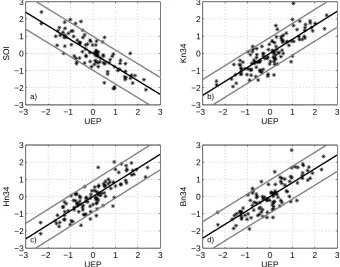
The correlation coefficients (R) between the UEP and SOI, Kn34, Hn34 and Bn34 are−0.81, 0.81, 0.82 and 0.81 respec-tively and each of these coefficients is statistically significant above the 99% confidence level (see Table 3 and Fig. 4). We note that the statistical significance of all correlation coeffi-cients presented in the study take into account serial (auto-) correlation in the series based on the reduced effective num-ber of degrees of freedom outlined by Davis (1976). These correlation coefficients are larger than any of the correlation
coefficients generated when comparing the 10 original input proxies versus observed indices of ENSO. Furthermore, us-ing a least squares linear regression model for each of the original ENSO proxies along with the new ENSO proxy we find the the new ENSO proxy has the smallest root mean square error (Table 3). Therefore, this confirms that the PCA analysis has acted to isolate the common ENSO related com-ponent of each of the original input proxies into PC1, our new ENSO proxy.
−3 −2 −1 0 1 2 3 −3
−2 −1 0 1 2 3
SOI
UEP a)
−3 −2 −1 0 1 2 3
−3 −2 −1 0 1 2 3
Kn34
UEP b)
−3 −2 −1 0 1 2 3
−3 −2 −1 0 1 2 3
Hn34
UEP c)
−3 −2 −1 0 1 2 3
−3 −2 −1 0 1 2 3
Bn34
UEP d)
Fig. 5. The least squares linear regression line (shown in black) between the UEP and the (a) SOI, (b) Kn34 SSTA, (c) Hn34 SSTA, and (d) Bn34 SSTA, while the gray lines indicate the 95% confidence interval.
Table 4. Direct correspondence of El Ni˜no (La Ni˜na) events between the unified ENSO proxy (UEP) and observations. Observed sources: SOI, Ropelewski and Halpert (1987); Kn34, Kaplan et al. (1998); Hn34, Rayner et al. (2003); Bn34, Bunge and Clarke (2009).
Correspondence SOI Kn34 Hn34 Bn34
Obs hits 74.2% (75.0%) 80.6% (74.2%) 75.8% (70.0%) 76.7% (70.6%)
Obs misses 25.8% (25.0%) 19.4% (25.8%) 24.2% (30.0%) 23.3% (29.4%)
UEP false events 20.6% (29.4%) 13.8% (32.3%) 13.8% (38.2%) 20.7% (29.4%)
standard deviations above or below the mean satisfies this criteria. This threshold value is roughly consistent with the Ni˜no 3.4 region SSTA threshold used for the definition of ENSO events by NOAA (which is 0.5◦C above or below the mean state, calculated from the period 1971–2000, where the standard deviation of observed Ni˜no 3.4 region SSTA for the period 1971–2000 is 0.93◦C).
The accuracy of the UEPs ability to capture discrete El Ni˜no and La Ni˜na events in the period 1878–1977 is then as-sessed. Using this 0.5 standard deviation threshold for ENSO events means that approximately 13of all years are classified as either El Ni˜no, La Ni˜na or Neutral. Looking at the corre-spondence between the UEP and observations we find that: (i) of the 31 (32) El Ni˜no (La Ni˜na) events identified in the SOI between 1878 and 1977 the UEP correctly identifies 23 (24); (ii) of the 31 (31) El Ni˜no (La Ni˜na) events identified in Kn34 between 1878 and 1977 the UEP correctly identifies 25 (23); (iii) of the 33 (30) El Ni˜no (La Ni˜na) events
iden-tified in Hn34 between 1878 and 1977 the UEP registers 25 (21) of these; and (iv) of the 30 (34) El Ni˜no (La Ni˜na) events identified in Bn34 between 1878 and 1977 the UEP registers 23 (24) of these (see Table 4 for more details). Hence, ap-proximately 77% of the El Ni˜no events and 72% of La Ni˜na events during the period 1878–1977 are captured by the UEP. Looking at the false alarm rate of the new ENSO proxy we find that there were: (i) 6 (10) false El Ni˜no (La Ni˜na) alarms raised that were not identified in the SOI; (ii) 4 (11) false El Ni˜no (La Ni˜na) alarms raised that were not identified in Kn34; (iii) 4 (13) false El Ni˜no (La Ni˜na) alarms raised that were not identified in Hn34; and (iv) 6 (10) false El Ni˜no (La Ni˜na) alarms raised that were not identified in Bn34. Consis-tent with other studies (e.g., Braganza et al. (2009)) the UEP shows higher skill in reproducing warm (El Ni˜no) events than the opposite phase.
1650 1700 1750 1800 Garcia08
Ortlieb00 Gergis09 Quinn92 UEP
Year
1850 1900 1950
Garcia08 Ortlieb00 Gergis09 Quinn92 UEP
Year
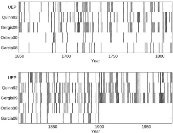
Fig. 6. Chronologies of El Ni˜no in the 1650–1978 period where vertical bars indicate the year0of the El Ni˜no event. Here the row labeled
UEP indicates El Ni˜no events identified in the UEP by the12 standard deviation threshold, while QN92 refers to Quinn and Neal (1992),
Orlieb00 refers to Ortlieb (2000), Garcia08 refers to Garcia-Herrera et al. (2008) and Gergis09 refers to Gergis and Fowler (2009).
proxies (using the same 0.5 standard deviation threshold to define El Ni˜no and La Ni˜na years), we find that the UEP cap-tures more El Ni˜no events in the observational period and has a lower false alarm rate than any of the original prox-ies. In regards to the La Ni˜na event capture, we find that the UEP again captures more events than any of the 10 origi-nal proxies. However, while the false alarm rate is relatively low at 16%, the false alarm rates of the Stahle et al. (1998), Mann et al. (2000) and Cook et al. (2008) ENSO proxies are slightly lower at 10%, 14% and 12%.
4.2 Comparison with historic ENSO chronologies
In this section we continue our assessment of the accu-racy of the UEPs ability to capture discrete El Ni˜no and La Ni˜na events. However, here instead of assessing the UEP against instrumental observations, we will be assessing the correspondence between the UEP and documented histori-cal chronologies of El Ni˜no (Quinn and Neal, 1992; Ortlieb, 2000; Garcia-Herrera et al., 2008; Gergis and Fowler, 2009) and La Ni˜na (Gergis and Fowler, 2009) events.
These historic chronologies of ENSO namely utilize doc-umentary sources of meteorological and climatic extremes from regions with weather conditions that are normally heav-ily influenced by ENSO events to provide a mainly binary type representation of ENSO variability. The most widely referenced of these chronologies is the El Ni˜no chronology of
Quinn and Neal (1992). This chronology, beginning in 1520 and ending in 1990, records El Ni˜no years charactorized by unusual climatic events in the South American region. The Quinn and Neal (1992) chronology has since been revised by Ortlieb (2000) to try and account for the ambiguity intro-duced into the Quinn record by using secondary documen-tary sources and climatic events in regions where weather is only weakly related to El Ni˜no. This revised work of Ortlieb (2000) covers the period 1520 through to and including the year 1900. The more recent documented historical El Ni˜no chronology of Garcia-Herrera et al. (2008), for the period 1550–1900, is based primarily on documentary records in Northern Peru. The final ENSO chronology used for verifica-tion in this study is that of Gergis and Fowler (2009). While the above chronologies all primarily used documentary evi-dence to assemble their chronologies, the study of Gergis and Fowler (2009) constructs a chronology of both El Ni˜no and La Ni˜na events using a combination of Paleoclimatic data and chronologies of ENSO variability. We note here that in cases when magnitude information is also included as part of the ENSO chronology, this extra information is disregarded and the information provided is simply used as binary type information.
Table 5. Direct and quasi-direct (in parentheses) correspondence between the unified ENSO proxy (UEP) and chronologies of El Ni˜no where QN92 = Quinn and Neal (1992), Orlieb00 = Ortlieb (2000), Garcia08 = Garcia-Herrera et al. (2008) and Gergis09 = Gergis and Fowler (2009). Quasi-direct correspondence counts direct correspondence along with events in the chronology that lag 1-yr behind the UEP El Ni˜no event.
Correspondence QN92 Ortlieb00 Garcia08 Gergis09
Obs hits 51.1% (75.5%) 29.0% (46.4%) 27.5% (47.8%) 69.1% (91.5%)
Obs misses 49.9% (24.5%) 71.0% (53.6%) 72.5% (52.2%) 30.9 (8.5%)
(69%) are registered in the Quinn and Neal (1992) (Gergis and Fowler, 2009) chronology (Fig. 6 and Table 5). Also, of the 110 La Ni˜na events identified in the UEP, 57.3% are reg-istered in the chronology of Gergis and Fowler (2009). As-sessing the direct correspondence between the UEP and the El Ni˜no chronologies of Ortlieb (2000) and Garcia-Herrera et al. (2008), over the period 1650–1900, we find that of the 75 El Ni˜no events registered in the UEP, approximately 29% and 28% are respectively registered in the Ortlieb (2000) and Garcia-Herrera et al. (2008) chronologies (Fig. 6 and Ta-ble 5). To assess the statistical significance of this corre-spondence we used a Monte Carlo type approach whereby we calculated 1000 Fourier based surrogates of the newly defined UEP using the method described by Theiler et al. (1992). These surrogates share the same mean, variance and power spectrum as the UEP, however, their phases are ran-domly shuffled. We then calculated the direct correspon-dence between each of these surrogates and the four El Ni˜no chronologies and one La Ni˜na chronology described above. We find that the correspondence between the UEP and the ENSO chronologies is statistically significant above the 99% level. Further to this, the correspondence between the UEP and these ENSO chronologies is larger than the correspon-dence between the ENSO chronologies and any of the 10 original ENSO proxies.
In order to get a more accurate representation of the UEP ENSO event capture we now make the assumption that the effects of UEP defined ENSO events could be felt in the ENSO chronologies in the year of the event or the year fol-lowing (quasi-direct correspondence). This allows for the ef-fects of annual averaging in the proxies and delayed ENSO teleconnections in the chronologies. For example, consider a typical El Ni˜no year, when taking an annual average of this events SSTA it is normally attributed to the year the event develops 0) instead of the year the event decays (year-1). Now, if we consider the climatic effects of this event, composite analysis reveals that El Ni˜no related South Amer-ican rainfall anomalies also straddle year 0 and year 1 (Ro-pelewski and Halpert, 1987). As such, a large rainfall event that occurred and was documented in the year after the event (year 1) could easily be attributed to the event in the year prior. Using this quasi-direct approach we find that the num-ber of corresponding El Ni˜no events between the UEP and the chronology of Quinn and Neal (1992) changes from 51%
to 75.5%, while the number of corresponding La Ni˜na events between the UEP and the chronology of Gergis and Fowler (2009) changes from 57.3% to 85.5% (Table 5). We note that while this jump in correspondence between the direct to quasi-direct is quite large, it is consistent with expecta-tions as this method essentially increases the degrees of free-dom of the relationship. Using the same Monte Carlo type approach as described in the paragraph above, we find that the quasi-direct correspondence between the UEP and each of the ENSO chronologies is again statistically significant above the 99% level. Furthermore, this quasi-direct corre-spondence between the UEP and these ENSO chronologies is also larger than the quasi-direct correspondence of any of the 10 original ENSO proxies.
5 ENSO variability since 1650
We have shown that the newly defined UEP provides an ac-curate representation of ENSO variability, and while it cor-responds well with the original proxy network, it provides a better representation of observed indices and documented historical chronologies of ENSO. Here we describe various changes in the UEP, and hence ENSO, which have occurred since 1650 focusing on (a) changes in ENSOs variance, (b) multi-year ENSO events, (c) multi-decadal variability, and (d) the effects of volcanic and solar forcing on ENSO.
5.1 Changes in ENSO variance
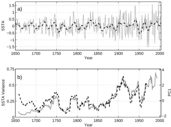
To assess the changes in ENSO variance since 1650 we calculate the variance of the UEP in a 16-yr running win-dow (Fig. 7b). However, prior to this the UEP variance is scaled to that of the HadSST1 annual mean (July–June) Ni˜no 3.4 region SSTA (Hn34) in the overlapping period us-ing UEP×σKn34
σUEP. The UEP is then extended to the year 2004
1650 1700 1750 1800 1850 1900 1950 2000 −1.5
−1 −0.5 0 0.5 1 1.5
Year
SSTA
a)
16500 1700 1750 1800 1850 1900 1950 2000
0.25 0.5 0.75
Year
SSTA Variance
b)
−2 0 2 4
PC1
Fig. 7. (a) The scaled UEP (gray) and its 13-yr low-pass filtered variability (black dashes); (b) The 16-yr running window variance of the scaled UEP is shown in gray while the first PC of the running variance of all 10 input proxies is shown in black dashes.
variance. They are, that the variance changes represent: (i) changed strength in the teleconnection patterns of ENSO; (ii) dating uncertainties within the source ENSO reconstructions, which if present generally increase back through time, re-ducing the amplitude of the common signal; (iii) proxy data quality problems; or (iv) real ENSO variability. Here, we will investigate each of these possible causes to try and as-certain whether these changes in variance represent the real ENSO signal.
Firstly, we note that there is high correspondence between the running variance of the UEP and that of the annual av-erage (July–June) of the verified Ni˜no 3.4 region SSTA of Bunge and Clarke (2009), where the correlation coefficient of 0.7 is statistically significant above the 99% level. As such the 20th century variance of the UEP is realistic. Secondly, while establishing the robustness of the UEP (see Methods section) 252 first PCs were generated from the 10choose5 network. To assess the robustness of the of these variance changes to the choice of input proxies used we calculated the 16-year running variance of each of these first PCs and com-pared it (by calculating the correlation coefficient) with that of the UEP. We find that all 252 correlation coefficients are statistically significant above the 99% level and larger than 0.83. Thus, the changes in UEP running variance are robust regardless of what proxies are selected from the original net-work (i.e., whether proxies are included that were calibrated to 20th century observations).
In regards to the effects of the changing strength of ENSO teleconnection patterns on ENSO reconstruction variance,
we have effectively reduced the effects of this by identify-ing the UEP in a network of ENSO reconstructions derived from globally distributed proxy data. The use of a PCA on the global proxy network diminishes the impact of regional specific changes in the signal by identifying the dominant changes in the entire network.
To identify the effects of proxy data quality problems we first analyze the variability amongst the 10 different input ENSO reconstructions. We would expect that if the quality of the proxy reconstructions were to deteriorate an increase in spread among the proxies would be seen. However, this is not apparent (Fig. 1b), so we do not believe that the quality of data systematically decays throughout the period 1650– 1977.
0 5 10 15 20 a)
0 5 10 15 20 25 b)
0 5 10 15 20 c)
0 5 10 15
ENSO count
d)
0 5 10 15 e)
0 5 10 15 20 f)
1550 1600 1650 1700 1750 1800 1850 1900 19500 5
10 15 20 g)
Year
Fig. 8. The number of El Ni˜no (red) and La Ni˜na (blue) events in a 30-yr centered running window from (a) the UEP (using a 0.5 stan-dard deviation threshold for ENSO events), the historical chronolo-gies of (b) Gergis and Fowler (2009), (c) Quinn and Neal (1992), (d) Ortlieb (2000), (e) Garcia-Herrera et al. (2008), and the proxy records of Bo¨es and Fagel (2008) and Hendy et al. (2003) which again use a 0.5 standard deviation threshold for El Ni˜no events.
running variance do diverge near the beginning of the record indicating that dating uncertainties begin to become impor-tant.
This suggests that the changes in variance of the UEP rep-resent a real signal in the original ENSO reconstructions. We now assess these changes in UEP variance with historic doc-umentary and unused paleo proxies to further verify the re-alism of these variance changes. We find that both the in-creasing trend in variance and the low variance period from 1650–1720 are supported by the 4 historical documentary chronologies of El Ni˜no variability already discussed in this study (Quinn and Neal, 1992; Ortlieb, 2000; Garcia-Herrera
1 2 3 4 5 6
0 10 20 30 40
Duration in years
Number of events
El Nino La Nina
Fig. 9. The number of ENSO events that persist un-interrupted for 1-6-yrs.
et al., 2008; Gergis and Fowler, 2009). In regards to the in-creasing trend in variance, there is a statistically significant (above the 95% level) linear increasing trend in the number of El Ni˜no events that occur in the 30-yr running windows in the period starting 1650 and ending at the end of each record of the four chronologies (Fig. 8b–e). While in regards to the low variance period of the late 17th century each of these chronologies displays a reduction in the number of El Ni˜no events during this period (Fig. 8b–e). It is not likely that the decreasing number El Ni˜no events back to this period or the low levels in the late 1600s are due to lack of documentation as all chronologies show a larger number of El Ni˜no events in the period prior to 1650.
1875 1900 1925 1950 1975 −3
−2 −1 0 1 2 3
Year
Fig. 10. The normalized 13-yr low-pass filtered time series of the UEP (gray) and PDO (black) along with time series of the IPO (black dashes).
5.2 Multi-year ENSO events
In the early 1990s the tropical Pacific Ocean displayed large scale El Ni˜no-like conditions which persisted for 5-yrs. So unusual was this event in the observational record that manuscripts discussing or seeking to understand this vari-ability became prevalent in the scientific literature (Kessler and McPhaden, 1995; Trenberth and Hoar, 1996; Latif et al., 1997). The title of Latif et al. (1997) explains the range of possible forcing mechanisms discussed in the scientific literature, “Greenhouse warming, Decadal variability, or El Ni˜no? An attempt to understand the anomalous 1990s”. In-terestingly, given the observations of the 20th century the study of Trenberth and Hoar (1996) estimates that the pro-longed 1990–1995 El Ni˜no event should occur once in about 1500–3000 years. Here, we use the newly defined ENSO proxy, the UEP, and a half standard deviation threshold to classify ENSO events, to examine just how unusual this multi-year behavior was in the context of ENSO variability of the last 350-yrs. To this end, we calculate the number of times in the UEP record (between 1650–1977) that El Ni˜no (La Ni˜na) conditions persist for 1 through to 6 consecutive years (Fig. 9). We find 7 (4) occurrences of El Ni˜no (La Ni˜na) events that persisted for 3 years and 1 (3) occurrences of El Ni˜no (La Ni˜na) events that persisted for 4 years. The multi-year El Ni˜no events (persisting for 3 or more years) occur reasonably frequently with approximately 2–3 events occurring every 100-yrs, with only the 1600s not displaying multi-year El Ni˜no events. It is a similar story for multi-year La Ni˜na events with 2–3 events occurring every 100-yrs and the 1600s not displaying any persistent negative events. Fur-ther to this, we find one occurrence of both El Ni˜no and La Ni˜na events that persist for 6 consecutive years in the 328 year record. Hence, while the prolonged El Ni˜no event of the early 1990s was unusual, it is neither a one off, nor the longest El Ni˜no event on record.
5.3 Multi-decadal variability
The shift towards more El Ni˜no-like conditions in the 1980s and 90s and the two large magnitude El Ni˜nos of 1982/83 and 1997/98 generated a lot of interest in scientific com-munity with many studies trying to ascertain the causes of this unusual period. While anthropogenic climate change was suggested as one of the possible mechanisms (Trenberth and Hurrell, 1994; Latif et al., 1997), the realization that this change in the late 1970s was one of several large changes that occurred during the 20th century (Trenberth and Hur-rell, 1994; Zhang et al., 1997) led a large number of studies to focus on how much of this apparent shift can be explained by a naturally occurring multi-decadal signal. This Pacific Ocean multi-decadal signal of the 20th century is represented by either the Pacific Decadal Oscillation (PDO) of Mantua et al. (1997), which is the North Pacific Ocean’s principal mode of decadal variability, or the Interdecadal Pacific Os-cillation (IPO) of Power et al. (1999), which is thought of as the Pacific-wide representation of the PDO (Folland et al., 2002).
More recent literature has questioned the statistical robust-ness of the IPO/PDO as a climate mode, raising the pos-sibility that the PDO/IPO could simply represent low fre-quency variability of ENSO (Rodgers et al., 2004; Schopf and Burgman, 2006). Regardless of its statistical robustness as a climate mode, it is an intriguing question whether such pronounced multi-decadal variability of the Pacific Ocean existed during the 250-yrs prior to the 20th century. In order to discuss the multi-decadal variability of the 20th century in the context of the last 350-yrs, we firstly validate the multi-decadal variability of the UEP (Fig. 7a) by comparing it with the multi-decadal variability of observed indices of ENSO, the IPO and PDO (Fig. 10) and the previously defined PDO reconstructions of Biondi et al. (2001) and D’Arrigo et al. (2001). Firstly, however, correlations between the multi-decadal variability of the UEP and the original input proxies are presented as a means to assess the contribution of each of the original input proxies to the low frequency variability of the UEP (Table 6). The relative magnitudes of these correla-tion coefficients are very similar to the relative weightings of the PCA (see Table 2), indicating that the low frequency vari-ability of the UEP represents the multi-decadal varivari-ability of the majortity of the original input recontructions.
low-frequency variability of the UEP over the period 1900– 1980, we find correlation coefficient of 0.75 which is again statistically significant above the 99% level. Comparing the multi-decadal variability of the UEP with the multi-decadal variability of two previously identified PDO proxies (Biondi et al., 2001; D’Arrigo et al., 2001), we find statistically sig-nificant (above the 95% level) correlation coefficients of 0.40 and 0.59 respectively. Thus, it appears that the UEP dis-plays multi-decadal variability that is consistent with the 20th century variability of ENSO indices, the PDO and IPO, as well as previously defined reconstructions of the PDO. As such, the UEP also provides a means to reconstruct the multi-decadal variability of the Pacific Ocean since 1650.
Focusing now on the PDO/IPO-like multi-decadal vari-ability of the last 350-yrs we will assess whether this multi-decadal variability has occurred throughout the last 350-yrs. We will then also use the UEP and its low frequency com-ponent to analyze whether phase of the PDO/IPO-type vari-ability is related to the variance of ENSO as suggested by the work of Kirtman and Schopf (1998) and Federov and Phi-lander (2000). Firstly, we find significant decadal variabil-ity has persisted throughout the last 350-yrs (Fig. 7a) with only a gradual reduction in the 60-yr running variance occur-ring (figure not shown). As such, there are numerous periods dominated by multi-decadal El-Ni˜no-like (La Ni˜na-like) be-havior like the period from 1830–1860 (1750–1790). If we now bin high frequency values of the UEP (calculated as the residual when the low-frequency UEP is subtracted from the UEP) according to the phase of the low frequency component we do not find a significant relationship between the phase of the PDO/IPO-type multi-decadal variability and variance of the UEPs high frequency variability. This result is consistent with the work of Yeh and Kirtman (2005).
5.4 The influence of Solar and Volcanic forcing
Solar variability and explosive volcanic events are both mechanisms that can alter the natural radiative forcing of the climate system. The previous studies of Clement et al. (1996); Cane et al. (1997); Mann et al. (2005) refer to an ocean dynamic thermostat mechanism whereby the tempera-ture of the eastern equatorial Pacific varies negatively with changes in radiative forcing. The study of Meehl et al. (2009) discusses the joint effects of the top-down strato-spheric ozone mechanism and the bottom-up coupled air-sea mechanism which cools the equatorial Pacific in response to peaks in solar forcing. Changes in radiative forcing have also been proposed to modulate the variance of ENSO (Mann et al., 2005), whereby low solar forcing periods are proposed to have higher ENSO variance. Using the UEP along with records of solar variability and volcanic forcing we will ex-amine whether the associated radiative forcing plays any role in the mean state or variability changes of ENSO in the last 350-yrs.
Table 6. Correlation coefficient between the 13-year lowpass fil-tered (LPF) Unified ENSO proxy (UEP) and the 13-year lowpass filtered original proxy network during the overlapping period. Sta-tistical significance of greater than the 99% (90%) level in the cor-relation coefficients is indicated by bold font (italic font).
Correlation LPF UEP
LPF Proxy 1 0.76
LPF Proxy 2 0.80
LPF Proxy 3 0.85
LPF Proxy 4 0.78
LPF Proxy 5 0.10
LPF Proxy 6 0.50
LPF Proxy 7 0.67
LPF Proxy 8 0.76
LPF Proxy 9 0.87
LPF Proxy 10 0.36
−2 −1 0 1 2 3 4 5 −3
−2 −1 0 1 2 3
Normalised SSTA
Year after Eruption
a)
−2 −1 0 1 2 3 4 5
−3 −2 −1 0 1 2 3
Normalised SSTA
Year after Eruption
b)
Fig. 11. Composites of the UEP around years in which explosive volcanism occurred where volcanic events are defined using the (a) IVI and (b) ICI indices. The solid black line indicates the composite mean while the gray dashed line indicates the composite median.
Consistent with the thermostat mechanism, past studies have suggested that explosive volcanic events (which reduce radiative forcing) tend to lead to a higher probability of El Ni˜no type events in the years following the eruption (Adams et al., 2003). Here we reassess these findings over the pe-riod 1650–1977 using the UEP, the ice-core volcanic index (IVI) of Gao et al. (2008) and the ice-core index (ICI) of vol-canic events by Crowley et al. (2008). To this end, both the IVI and ICI data were then discretized into a binary format where 1’s (0’s) indicate whether a volcanic event occurred (did not occur) in the given year. A subset of the UEP data was then made which incorporated an eight year window of data from the UEP (consisting of the 2-yrs prior to the event, the event year and the 5-yrs following the event) for each of the recorded volcanic events. Visual analysis of these data subsets reveals two distinct features, (i) a shift in the data towards more El Ni˜no like conditions in the year of the vol-canic eruption, and (ii) a shift in the data towards more La Ni˜na like conditions approximately 2–3 years after the vol-canic eruption (Fig. 11). Both of these features are consis-tent with Adams et al. (2003) and not inconsisconsis-tent with the results expected from the thermostat mechanism of Clement et al. (1996).
We now specifically test the null hypothesis: volcanic forc-ing has no effect on the mean state, median or probability of ENSO in the years during or surrounding the volcanic event. We find that the distribution of the UEP shifts toward more El
Ni˜no-like state the year both the IVI or the ICI mark an erup-tion event. Two statistical tests support the significance of the shifts: the t-test (which shows that the change in mean state is significant above the 95% level), and the Mann-Whitney U-test (which shows that the change in the median is stati-cally significant above the 95% level) (Fig. 11). However, while the shift towards a La Ni˜na like mean state 2–3 years after the volcanic event is apparent in both data subsets, the shift in mean state and the median in either data subset is not statistically significant.
eruptions act to significantly alter the mean state and median of ENSO while also significantly altering the probability of ENSO events occurring. Hence, the null hypothesis can be rejected with some degree of confidence.
6 Discussion and conclusions
In this manuscript we defined a new proxy of ENSO variabil-ity covering the last 3 1/2 centuries, titled the “Unified ENSO Proxy” (UEP). The UEP uses a PCA to combine the joint sig-nal in the 10 selected, previously defined, reconstructions of ENSO (Dunbar et al., 1994; Stahle et al., 1998; Cook, 2000; Mann et al., 2000; Evans et al., 2001, 2002; Cobb et al., 2003; Cook et al., 2008; Braganza et al., 2009). This results in a robust ENSO index which displays an enhanced correspon-dence with observations during the last century and with his-torical chronologies of ENSO over the entire period. We note here that each of the individual ENSO reconstructions used as input for this manuscript could be affected by the changing strength of ENSO teleconnections, dating uncertainties, bio-logical biases, regional climatic factors and other non-ENSO related large scale climatic modes. As such, so could the UEP. However, each of the input reconstructions used that was derived from multiple site proxies were processed by the generating authors in order to extract the ENSO signal away from this unrelated noise (Stahle et al., 1998; Cook, 2000; Mann et al., 2000; Evans et al., 2001, 2002; Braganza et al., 2009). Additionally, here we carry out a PCA on these pre-processed ENSO reconstructions, derived from a global proxy network, which acts to further reduce the potential er-rors due to site specific ENSO reconstruction biases.
Upon analysis of the UEP, the feature that stands out most is the increase in variance through time. This feature is well represented by the dominant mode of running mean variance of the 10 original input proxies, meaning that it is a fea-ture in the majority of the input proxies. Further to this, it appears consistent with historic chronologies of ENSO and three separate un-utilized proxies of ENSO variability. As to the cause of this increase in variance, it is still an open ques-tion. Interestingly though, this increase in ENSO variance roughly coincides with an increase in Western Pacific warm pool temperature (Newton et al., 2006). Consistent with the ENSO variance changes displayed by the UEP, the increas-ing temperature of the Western Pacific warm pool should lead to enhanced ENSO variance, provided the subsurface ocean remains at the same temperature (Sun, 2000). It was also recently reported that the Inter-tropical Convergence Zone (ITCZ) migrated northward between the year 1700 and 1850 (Sachs et al., 2009). The effect the northward migration of the ITCZ would have on the variance of ENSO is unclear at this stage. For instance, numerous studies conjecture that the northward (southward) migration of the ITCZ should lead to decreased (increased) ENSO variance (Haug et al., 2001; Koutavas and Lynch-Stieglitz, 2004). However, model
evi-dence from the perpetual month experiments of Tziperman et al. (1997) (where the Zebiak and Cane (1987) anomaly models background annual cycle winds, ocean currents and the associated ITCZ position are held fixed) is inconclu-sive as it indicates that ENSO is extremely damped when the ITCZ is both at its northern and southern most extremes in September and February respectively. To further explore the role of Western Pacific warm pool temperature changes and the northward migration of the ITCZ on the variance of ENSO, future work will investigate the associated changes in zonal convection, flow divergence, thermal damping, Ekman pumping and thermocline feedbacks by computing the sea-sonally varying BJ index (Jin et al., 2006) of climate models subject to modified WPWP temperature and ITCZ latitude.
Using the UEP we also analyzed several topical issues in the ENSO literature, the occurrence of multi-year El Ni˜no events, multi-decadal variability and the effects of solar and volcanic forcing. In regards to multi-year or prolonged ENSO events, a study by Trenberth and Hoar (1996) esti-mated the prolonged El Ni˜no event of the early 1990s, which persisted for 5-yrs by some measures, would only occur once in approximately 1500–3000-yrs. Using the newly defined ENSO proxy, the UEP, and a half standard deviation thresh-old to classify ENSO events, we find that while the prolonged El Ni˜no event of the early 1990s was unusual, it is neither a one off and or the longest El Ni˜no event on record. Prolonged ENSO events have occurred at least several times over the last 3 12 centuries, with El Ni˜no events that persist for 3 or more years generally occurring 2–3 times per century.
Acknowledgements. This work is supported by NOAA’s CCDD
program under grant number NA08OARH320910. The UEP
and its low-pass filtered decadal component is made available on the World Data Center (WDC) for paleoclimatology and the Asia-Pacific Data Research Center (APDRC).
Edited by: B. L. Otto-Bliesner
The publication of this article was sponsored by PAGES.
References
Adams, J., Mann, M. E., and Ammann, C. M.: Proxy evidence for an El Ni˜no-like response to volcanic forcing, Nature, 426, 274– 278, 2003.
Biondi, F., Gershunov, A., and Cayan, D. R.: North Pacific Decadal Climate Variability since 1661, J. Climate, 14, 5–10, 2001. Bo¨es, X. and Fagel, N.: Relationships between southern Chilean
varved lake sediments, precipitation and ENSO for the last 600 years, J. Paleolimnol., 39, 237–252, doi:10.1007/s10933-007-9119-9, 2008.
Braganza, K., Gergis, J. L., Power, S. B., Risbey, J. S., and Fowler, A. M.: A multiproxy index of the El Ni˜no-Southern Oscillation, A.D. 1525–1982, J. Geophys. Res., 114, D05106, doi:10.1029/2008JD010896, 2009.
Bunge, L. and Clarke, A. J.: A verified estimation of the El Ni˜no index NINO3.4 since 1877, J. Climate, 22, 3979–3992, 2009. Cane, M., Clement, A. C., Kaplan, A., Kushnir, Y., Pozdnyakov,
D., Seager, R., Zebiak, S. E., and Murtugudde, R.: Twentieth-century sea surface temperature trends, Science, 275, 957–960, 1997.
Chan, J.: Tropical cyclone activity in the northwest Pacific in re-lation to the El Ni˜no/Southern Oscilre-lation phenomenon, Mon. Weather Rev., 113, 599–606, 1985.
Clement, A., Seager, R., Cane, M. A., and Zebiak, S. E.: An ocean dynamical thermostat, J. Climate, 9, 2190–2196, 1996.
Cobb, K., Charles, C. D., Cheng, H., and Edwards, R. L.: El Ni˜no-Southern Oscillation and tropical Pacific climate during the last millenium, Nature, 424, 271–276, 2003.
Conroy, J. L., Restrepo, A., Overpeck, J. T., Steinitz-Kannan, M., Cole, J. E., Bush, M. B., and Colinvaux, P. A.: Unprecedented recent warming of surface temperatures in the eastern tropical Pacific Ocean, Nat. Geosci., 2, 46–50, doi:10.1038/NGEO390, 2009.
Cook, E.: Ni˜no 3 Index Reconstruction, in: International Tree-Ring Data Bank, IGBP PAGES/World Data Center-A for Paleoclima-tology Data Contribution Series, 2000.
Cook, E. R., D’Arrigo, R. D., and Anchukaitis, K. J.: ENSO recon-structions from long tree-ring chronologies: Unifying the dif-ferences, in: Talk presented at a special workshop on Reconcil-ing ENSO Chronologies for the Past 500 Years, held in Moorea, French Polynesia on 2–3 April 2008, 2008.
Crowley, T. J., Zielinski, G., Vinther, B., Udisti, R., Kreutz, K., Cole-Dai, J., and Castellano, E.: Volcanism and the Little Ice Age, PAGES news, 16, 22–23, 2008.
D’Arrigo, R., Villalba, R., and Wiles, G.: Tree-ring estimates of Pacific Decadal Climate Variability, Clim. Dynam., 18, 219–224, 2001.
Davis, R.: Predictability of Sea Surface Temperature and Sea Level Pressure anomalies over the North Pacific Ocean, J. Phys. Oceanogr., 6, 249–266, 1976.
Dunbar, R., Wellington, G. M., Colgan, M. W., and Glynn, P. W.: Eastern Pacific sea surface temperature since 1600 A.D.: The
δ18O record of climate variability in Gal´apagos corals,
Paleo-ceanography, 9, 291–315, 1994.
Emile-Geay, J., Cane, M. A., Seager, R., Kaplan, A., and Almasi, P.: El Ni˜no as a mediator of the solar influence on climate, Pale-oceanography, 22, PA3210, doi:10.1029/2006PA001304, 2007. Evans, M., Kaplan, A., Cane, M. A., and Villalba, R.:
Interhemi-spheric Climate Linkages, chap. Globality and optimality in cli-mate field reconstructions from proxy data, Cambridge Univer-sity Press, 53–72, 2001.
Evans, M., Kaplan, A., and Cane, M. A.: Pacific sea surface
temperature field reconstruction from coralδ18O data using
re-duced space objective analysis, Paleoceanography, 17, 1007, doi:10.1029/2000PA000590, 2002.
Federov, A. and Philander, S. G.: Is El Ni˜no changing?, Science, 288, 1997–2002, 2000.
Folland, C. K., Renwick, J. A., Salinger, M. J., and Mullan, A. B.: Relative influences of the Interdecadal Pacific Oscillation and ENSO on the South Pacific Convergence Zone, Geophys. Res. Lett., 29, 1643, doi:10.1029/2001GL014201, 2002.
Gao, C., Robock, A., and Ammann, C.: Volcanic forcing of cli-mate over the past 1500 years: An improved ice core-based index for climate models, J. Geophys. Res., 113, D23111, doi:10.1029/2008JD010239, 2008.
Garcia-Herrera, R., Diaz, H. F., Garcia, R. R., Prieto, M. R., Bar-riopedro, D., Moyano, R., and Hern´andez, E.: A chronology of El Ni˜no events from primary documentary sources in Northern Peru, J. Climate, 21, 1948–1962, doi:10.1175/2007JCLI1830.1, 2008.
Gergis, J. and Fowler, A. M.: A history of ENSO events since A.D. 1525: Implications for future climate change, Climatic Change, 92, 343–387, doi:10.1007/s10584-008-9476-z, 2009.
Haug, G. H., Hughen, K. A., Sigman, D. M., Peterson, L. C., and Rohl, U.: Migration of the Intertropical Convergence Zone through the Holocene, Science, 293, 1304–1308, 2001. Hendy, E., Gagan, M. K., and Lough, J. M.: Chronological
con-trol of coral records using luminescent lines and evidence for non-stationary ENSO teleconnections in northeast Australia, The Holocene, 13, 187–199, 2003.
Jin, F., Kim, S., and Bejarano, L.: A coupled-staibility
index for ENSO, Geophys. Res. Lett., 33, L23708,
doi:10.1029/2006GL027221, 2006.
Kaplan, A., Cane, M., Kushnir, Y., Clement, A., Blumenthal, M., and Rajagopalan, B.: Analyses of global sea surface temperature 1856–1991, J. Geophys. Res., 103, 567–589, 1998.
Kessler, W. and McPhaden, M.: The 1991–93 El Ni˜no in the Central Pacific, Deep-Sea Res. Pt. II, 42, 295–333, 1995.
Kirtman, B. and Schopf, P.: Decadal variability in ENSO pre-dictability and prediction, J. Climate, 11, 2804–2822, 1998. Koutavas, A. and Lynch-Stieglitz, J.: The Hadley Circulation:
Academic Publishers, Boston, 347–369, 2004.
Latif, M., Kleeman, R., and Eckert, C.: Greenhouse Warming, Decadal Variability, or El Ni˜no? An attempt to understand the anomalous 1990s, J. Climate, 10, 2221–2239, 1997.
Lean, J., Beer, J., and Bradley, R.: Reconstruction of Solar Irra-diance since 1610: Implications for Climate Change, Geophys. Res. Lett., 22, 3195–3198, 1995.
Mann, M., Bradley, R. S., and Hughes, M. K.: Multiscale Variabil-ity and Global and Regional Impacts, chap. Long-term variabilVariabil-ity in the El Ni˜no-Southern Oscillation and asscoiated teleconnec-tions, Cambridge University Press, 357–412, 2000.
Mann, M., Cane, M. A., Zebiak, S. E., and Clement, A.: Vol-canic and Solar Forcing of the Tropical Pacific over the Past 1000 Years, J. Climate, 18, 447–456, 2005.
Mantua, N., Hare, S. R., Zhang, Y., M.Wallace, J., and Francis, R. C.: A Pacific interdecadal climate oscillation with impacts on salmon production, B. Am. Meteorol. Soc., 78, 1069–1079, 1997.
Meehl, G. A., Arblaster, J. M., Matthes, K., Sassi, F., and van Loon, H.: Amplifying the Pacific Climate System response to a small 11-year Solar Cycle forcing, Science, 325, 1114–1118, doi:10.1026/science.1172872, 2009.
Merryfield, W. J.: Changes to ENSO under CO2 doubling in a mul-timodel ensemble, J. Climate, 19, 4009–4027, 2006.
Newton, A., Thunell, R., and Stott, L.: Climate and
hy-drographic variability in the Indo-Pacific Warm Pool dur-ing the last millenium, Geophys. Res. Lett., 33, L19710, doi:10.1029/2006GL027234, 2006.
Nicholls, N.: Predictability of interannual variations of Australian seasonal tropical cyclone activity, Mon. Weather Rev., 113, 1144–1149, 1985.
Ortlieb, L.: Multiscale Variability and Global and Regional Im-pacts, chap. The documented historical record of El Ni˜no events in Peru: An update of the Quinn Record (Sixteenth through Nine-teenth Centuries), Cambridge University Press, 207–295, 2000. Power, S. and Smith, I. N.: Weakening of the Walker Circulation
and apparent dominance of El Ni˜no both reach record levels, but has ENSO really changed?, Geophys. Res. Lett., 34, 18702, doi:10.1029/2007GL030854, 2007.
Power, S., Casey, T., Folland, C., Colman, A., and Mehta, V.: Inter-decadal modulation of the impact of ENSO on Australia, Clim. Dynam., 15, 319–324, 1999.
Quinn, W. and Neal, V. T.: Climate since A.D. 1500, chap. The historical record of El Ni˜no events, Routledge, 623–648, 1992. Rayner, N., Parker, D., Horton, E., Folland, C., Alexander, L.,
Rowell, D., Kent, E., and Kaplan, A.: Global analyses of sea surface temperature, sea ice, and night marine air temperature since the late nineteenth century, J. Geophys. Res., 108, 4407, doi:10.1029/2002JD002670, 2003.
Rodgers, K., Friedrichs, P., and Latif, M.: Tropical Pacific Decadal Variability and Its Relation to Decadal Modulations of ENSO, J. Climate, 17, 3761–3774, 2004.
Ropelewski, C. F. and Halpert, M. S.: Global and Regional precipi-tation patterns associated with the El Ni˜no/Southern Oscillation, Mon. Weather Rev., 115, 1606–1626, 1987.
Sachs, J. P., Sachse, D., Smittenberg, R. H., Zhang, Z., Battisti, D. S., and Golubic, S.: Southward movement of the Pacific in-tertropical convergence zone AD 1400–1850, Nat. Geosci., 2, 519–525, doi:10.1038/NGEO554, 2009.
Schopf, P. S. and Burgman, R. J.: A simple mechanism for ENSO residuals and asymmetry, J. Climate, 19, 3167–3179, 2006. Stahle, D., D’Arrigo, R. D., Krusic, P. J., Cleaveland, M. K.,
Cook, E. R., Allan, R. J., Cole, J. E., Dunbar, R. D., Therrell, M. D., Gay, D. A., Moore, M. D., Stokes, M. A., Burns, B. T., Villanueva-Diaz, J., and Thompson, L. G.: Experimental den-droclimatic reconstruction of the Southern Oscillation, B. Am. Meteorol. Soc., 79, 2137–2152, 1998.
Sun, D.-Z.: Multiscale Variability and Global and Regional Im-pacts, chap. Global Climate Change and El Ni˜no: A theoretical framework, Cambridge University Press, 443–463, 2000. Theiler, J., Eubank, S., Longtin, A., Galdrikian, B., and Farmer,
J. D.: Testing for nonlinearity in time series: the method of sur-rogate data, PhysicaD, 58, 77–94, 1992.
Timmermann, A.: Detecting the nonstationary response of ENSO to Greenhouse Warming, J. Atmos. Sci., 56, 2313–2325, 1999. Trenberth, K. and Hoar, T. J.: The 1990-1995 El Ni˜no-Southern
Oscillation event: Longest on record, Geophys. Res. Lett., 23, 57–60, 1996.
Trenberth, K. and Hurrell, J. W.: Decadal atmosphere-ocean varia-tions in the Pacific, Clim. Dynam., 9, 303–319, 1994.
Trenberth, K. E. and Stepaniak, D. P.: Indices of El Ni˜no Evolution, J. Climate, 14, 1697–1701, 2001.
Tziperman, E., Zebiak, S. E., and Cane, M. A.: Mechanisms of Seasonal – ENSO interaction, J. Atmos. Sci., 54, 61–71, 1997. van Oldenborgh, G. J., Philip, S. Y., and Collins, M.: El Ni˜no in
a changing climate: a multi-model study, Ocean Sci., 1, 81–95, 2005,
http://www.ocean-sci.net/1/81/2005/.
von Storch, H. and Zwiers, F. W.: Statistical Analysis in Climate Research, Cambridge University Press, 2000.
Yeh, S.-W. and Kirtman, B. P.: Pacific Decadal Variability and ENSO amplitude modulation, Geophys. Res. Lett., 32, L05703, doi:10.1029/2004GL02173, 2005.
Zebiak, S. E. and Cane, M. A.: A model El Ni˜no-Southern Oscilla-tion, Mon. Weather Rev., 115, 2262–2278, 1987.