www.atmos-meas-tech.net/9/4141/2016/ doi:10.5194/amt-9-4141-2016
© Author(s) 2016. CC Attribution 3.0 License.
Estimates of Mode-S EHS aircraft-derived wind observation errors
using triple collocation
Siebren de Haan
KNMI, Wilhelminalaan 10, De Bilt 3732 GK, the Netherlands
Correspondence to:Siebren de Haan ([email protected])
Received: 15 November 2015 – Published in Atmos. Meas. Tech. Discuss.: 3 December 2015 Revised: 22 April 2016 – Accepted: 26 May 2016 – Published: 30 August 2016
Abstract.Information on the accuracy of meteorological ob-servation is essential to assess the applicability of the mea-surements. In general, accuracy information is difficult to obtain in operational situations, since the truth is unknown. One method to determine this accuracy is by comparison with the model equivalent of the observation. The advan-tage of this method is that all measured parameters can be evaluated, from 2 m temperature observation to satellite ra-diances. The drawback is that these comparisons also con-tain the (unknown) model error. By applying the so-called triple-collocation method (Stoffelen, 1998), on two indepen-dent observations at the same location in space and time, combined with model output, and assuming uncorrelated observations, the three error variances can be estimated. This method is applied in this study to estimate wind ob-servation errors from aircraft, obtained utilizing informa-tion from air traffic control surveillance radar with Selective Mode Enhanced Surveillance capabilities (Mode-S EHS, see de Haan, 2011). Radial wind measurements from Doppler weather radar and wind vector measurements from sodar, together with equivalents from a non-hydrostatic numerical weather prediction model, are used to assess the accuracy of the Mode-S EHS wind observations. The Mode-S EHS wind (zonal and meridional) observation error is estimated to be less than 1.4±0.1 m s−1 near the surface and around 1.1±0.3 m s−1at 500 hPa.
1 Introduction
Quantifying observation errors is of major importance to cor-rectly use or interpret the measured information. For exam-ple, the optimal use of observations in assimilation, using
(2.45 ms−1 for Mode-S EHS and 2.12 ms−1for AMDAR). The accuracies found in these studies were relative to the other observed measurements (or model) and include these errors. The real error with respect to the truth is hard (if not impossible) to measure.
A method to avoid the information on the truth while estimating the uncertainty of three collocated observations in space and time was developed by Stoffelen (1998). The only requirement on the three data sets is that they are not correlated. Most triple-collocation data sets consist of two measurement systems and a numerical weather prediction (NWP) model. Several studies have been performed using this method (Vogelzang et al., 2011; Roebeling et al., 2012; Draper et al., 2013) for different kinds of observation. In this paper the observation error of wind measurements from Mode-S EHS, based on triple collocation with NWP and so-dar or raso-dar, will be presented.
Although radiosonde observations are regarded as a refer-ence in meteorology, these observations are not exploited in this study. At present, due to budget cuts, only one launch per day at 00:00 UTC is performed. At that time the number of aircraft landing at or departing from Schiphol airport is very low (i.e. 01:00 LT or 02:00 LT depending on summer-or wintertime), and thus this will hamper the number of col-locations, especially in the boundary layer. Furthermore, the distance between the radiosonde launch site (De Bilt) and the airport is more than 30 km. Nevertheless, radiosonde obser-vations are a valuable source for detecting model deficien-cies (see e.g. Houchi et al., 2010). The sodar is installed at Schiphol airport.
This paper is organized as follows. In Sect. 2 the data are described. In Sect. 3, the methodology is discussed; that is, the triple-collocation method, the method of collocation, and the assumptions made are described. The results of the triple collocation are presented in Sect. 4. The last section is dedi-cated to the conclusions and outlook.
2 Data
In this section the data sources used in the present study are described. First a description is given of Mode-S EHS obser-vations, followed by radar and sodar. The used NWP model is described last.
2.1 Aircraft-derived data (Mode-S EHS)
Aircraft are equipped with sensors for flight efficiency and safety. For this purpose, an aircraft measures the speed of the aircraft, its position, and ambient temperature and pressure. For a few decades a selection of these observations are trans-mitted to a ground station using the AMDAR system. An at-mospheric profile can be generated when measurements are taken during take-off and landing. See Painting (2003) for more details. Recently, a new type of aircraft-related
meteo-rological information has become available, which originates from observations inferred from a tracking and ranging radar used for air traffic control. These data are called Mode-S EHS because they use the Selective EnHanced Surveillance Mode of the radar (de Haan, 2011)1. Mode-S EHS observations are received through the aircraft surveillance system triggered by a secondary surveillance radar (SSR) to track and interrogate aircraft. The SSR sends a request for information on for ex-ample aircraft identification, heading, and air speed. From this information wind and temperature information can be derived from the position of the aircraft reported by heading, ground track, and true air speed. Heading is the direction the nose of the aircraft points to; true air speed is the speed of the aircraft with respect to air, and the ground track is the motion of the aircraft relative to the ground. The wind vec-tor is the difference between the motion of the aircraft rela-tive to the ground and its motion relarela-tive to the air (defined by the airspeed and heading). To obtain high-quality wind information, the heading and airspeed are corrected as de-scribed in de Haan (2011, 2013). The derived temperatures are of lower quality due to the method of derivation de Haan (2011). Another method to derive temperature information has been developed by Stone and Kitchen (2015) where the height and pressure information available in Automatic De-pendent Surveillance Broadcast (ADS-B) was exploited to estimate a layer temperature. They found that a mean-layer temperature of a 2 km thick mean-layer can be obtained with an error of around 1 K.
An SSR has a typical interrogation frequency of once ev-ery 4 to 20 s. Consequently, wind and temperature are ob-served at these same rates, and with a typical cruising speed of 250 m s−1 the horizontal resolution of these data is be-tween 1 and 5 km, for a single tracking radar. Note that data points are removed by quality control, related to for example turning of the aircraft. Nevertheless a large number of obser-vation pass quality control (about 20 %). See de Haan (2011, 2013) for more details.
The difference between Mode-S EHS and AMDAR lies in the method of retrieving the data. AMDAR data are transmit-ted through a dedicatransmit-ted relay system, and AMDAR obser-vations are initiated on request of the meteorological com-munity. Not all aircraft are AMDAR equipped; only selected aircraft have the AMDAR software implemented on their on-board computer.
The focus of this paper is on wind, although (mean-layer) temperature is also available in Mode-S EHS or ADS-B information; temperature will be investigated in future re-search.
2.2 Radar and sodar
A Doppler weather radar is capable of determining one com-ponent of the velocity of scattering particles. Only the
locity component along the line of sight, the so-called ra-dial velocity, can be determined. A Doppler radar is com-monly associated with measurements of frequency shifts be-cause of the low velocities of hydrometeors. However, these shifts cannot be observed directly. The phase of the scattered electromagnetic waves is employed to determine the Doppler frequency shift instead. During pulse-pair processing, the ve-locity is effectively deduced from the phase jump of the re-ceived signal. The unambiguous velocity interval of the in-strument, especially for C-band radars, is enhanced by apply-ing a dual-pulse repetition frequency (PRF). The two Royal Netherlands Meteorological Institute (KNMI) radars are C-band with a wavelength of 5.3 cm. The high PRF is chosen to be four-thirds of the low PRF, resulting in an unambigu-ous velocity of 4 times the low PRF unambiguunambigu-ous velocity, which is 23 m s−1for the lowest elevations and 47 m s−1for the highest elevations. The PRF also determines the unam-biguous range of the radar, which is 240 km for the lowest elevations and reducing to 120 km for the highest elevations. The radar beam will have an increasing height with increas-ing distance to radar due to the curvature of the earth.
A sodar (sonic detection and ranging) is a ground-based remote-sensing instrument for measuring wind and turbu-lence in the lower atmosphere. A mono-static sodar is op-erated and maintained by KNMI at Amsterdam Airport Schiphol (AAS) since March 2006. A sodar emits short acoustic pulses into the atmosphere and receives atmospheric echoes generated by small-scale density fluctuations that are associated only with thermally driven turbulence, which is not always present. The transmitted signals can be phase shifted to point the beam in different directions. At Schiphol, three are in use for the instrument, and one antenna is ori-ented vertically. The zenith angle of the other beams is de-pendent on the transmit frequency and varies between 10 and 30◦. The distance of the measuring volume is deter-mined from the propagation time of the acoustic wave and the estimated acoustic velocity. Since the temperature inho-mogeneities move with the wind, a Doppler frequency shift is observed that makes it possible to derive the wind speed relative to the beam axis. By measuring the Doppler shift for different beam directions, the full 3-dimensional wind at spe-cific altitudes can be determined. Thereby it is assumed that the flow is horizontally homogeneous over the area contain-ing the different measurcontain-ing volumes.
2.3 NWP data
The non-hydrostatic HARMONIE (Hirlam ALADIN Re-search on Mesoscale Operational NWP in Euromed; Seity et al., 2011; Brousseau et al., 2011) model is the follow-up of the hydrostatic HIRLAM (HIgh Resolution Limited Area Model) model; HARMONIE explicitly resolves con-vective processes. The model grid size of the HARMONIE model version (cy38h1.2) operational at KNMI is 2.5 km, and the HARMONIE model has been available since early
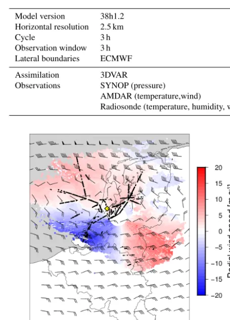
Table 1.HARMONIE main characteristics.
Model version 38h1.2 Horizontal resolution 2.5 km Cycle 3 h Observation window 3 h Lateral boundaries ECMWF
Assimilation 3DVAR
Observations SYNOP (pressure)
AMDAR (temperature,wind)
Radiosonde (temperature, humidity, wind)
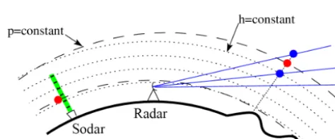
Figure 1.Radial wind speed from the Doppler weather radar in De Bilt, location of the sodar (marked by the yellow diamond), Mode-S EHS observations (black dots), and HARMONIE (thinned) wind field at approximately 850 hPa; all valid on 3 September 2013 12:00 UTC.
2012 at KNMI. The model domain covers mainly western Europe and part of the North Atlantic and the number of grid points is 800×800, meaning that the domain covers a 2000×2000 km2area. The number of model levels equals 65 with higher density in the lower part of the troposphere. The operational HARMONIE model version at KNMI is nested in the European Centre for Medium-Range Weather Forecasts (ECMWF) model. Note that lateral boundary con-ditions are ECMWF forecasts, generated from an (global) analysis using a large variety of observation types (SYNOP, radiosonde and satellite information). Table 1 lists the HAR-MONIE version used in the study and its main characteris-tics. In this study we will only use the 3 h forecast data.
Table 2 describes the main characteristics of the observa-tion data sets used in this study. Figure 1 shows an example of the wind data.
Table 2.Observation data characteristics.
Data type Horizontal Vertical Vertical Temporal resolution resolution range resolution Mode-S EHS 1–4 km variable surface–11 km 4–10 s Radar 1 km 100 m 500 m–8 km 5 min Sodar 1 km 25 m 50–700 m 15 min HARMONIE (FC+03) 2.5 km 50 m near surface surface–0.1 hPa 3 h
1 km above 3 km
3 Methodology
To perform a triple collocation it is essential that the data sets are collocated in space and time. In this section the method of collocation is described followed by the description of the triple-collocation methodology.
3.1 Collocation algorithm
Observations are regarded at the same when the time differ-ence is less than 5 min. Note that the model has a 3 h cycle (a new run is started every 3 h), which reduces the collocation time window to 10 min every 3 h because we use the 3 h fore-cast only in this study. We did not interpolate the model to the observation time and the interpolation in space was chosen to be bilinear.
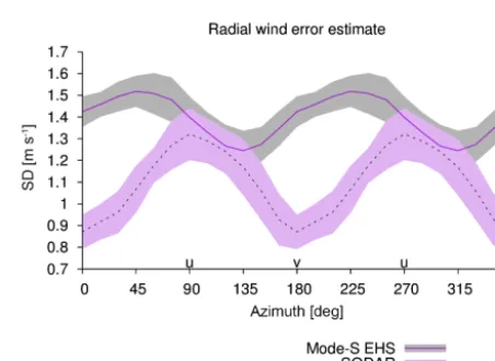
3.1.1 Radar and Mode-S EHS data collocation method The metrics of the vertical coordinate of radar and Mode-S EHS observation differ: radar radial winds are measured at a certain elevation angle and range, while altitude of Mode-S EHS is given as flight level. The elevation angle and range can be converted into position and altitude (in metres), while flight level is easily converted into pressure altitude (in hec-topascals). To enable collocation of a radar and Mode-S EHS observation, additional information on surface pressure, and temperature and humidity profile is needed to convert either pressure into altitude or vice versa. To perform this conver-sion, the surface pressure, and temperature and humidity pro-file of an NWP model is used, which is already present at the observation location since NWP is the third data set. This may introduce a correlation between the three data sets, but we think it is negligible. Figure 2 shows schematically the vertical collocation.
Given a Mode-S EHS observation location, a matching radar observation is determined by the following conditions. First of all the distance of the observation location should be at least 50 km away from the radar, because close to the radar the radial wind observations have a large error. The Mode-S EHS observation will not perfectly collocate to the altitude and position of a radar pixel; therefore, radar data points of two closest elevations with a maximal horizontal distance of 2.5 km are considered. Next, the elevation of the
surround-Figure 2.Schematic overview of the vertical collocation method. The dashed lines represent levels of constant pressure and the dot-ted lines of constant height. Red dots denote the Mode-S EHS ob-servation, the blue dots the collocated radar observation.
ing radar data points needs to be larger than 0.3◦(the lowest elevation angle) and smaller than 6◦. To avoid gross errors, quality checks are included to select a radar data point for triple collocation: at least 10 radar radial velocity observa-tions should be close to the Mode-S EHS location, and the standard deviation of these points needs to be smaller than 0.5 m s−1. This threshold was used in order to avoid gross er-rors in radial velocity due to for example ambiguity problems and clutter. One should note that very variable atmospheric conditions are also removed from the data set. The mean ra-dial velocity finally is used as a triple-collocation point when the mean altitude of the radar point is within 200 m of the Mode-S EHS altitude.
3.2 Triple collocation
We apply the triple-collocation method (Stoffelen, 1998) to find quantitative information on the observation error. This method exploits a data set consistent of three co-located mea-surements of the same parameter. In this paper we use two different wind data sets; the first consist of Mode-S EHS wind vector observation, sodar, and NWP at Schiphol air-port, and the second data set consists of Mode-S EHS, radar radial wind, and NWP. The triple-collocation method deter-mines simultaneously the linear calibration coefficients and the error of the three data sets under consideration. See Stof-felen (1998) and Vogelzang et al. (2011) for more details. Below, a brief description of the method is given.
Assume we have three sets of dataX1,X2, andX3, collo-cated in space and time, whereX1has the highest (expected) accuracy and X3 the lowest (expected) accuracy. Since the truth is unknown we take data setX1as the unbiased refer-ence (or truth). Assume furthermore that two other data sets have a linear relationship with this truth, that is
x1=t+1, (1)
x2=a2t+b2+2, (2)
x3=a3t+b3+3, (3)
wheret is the truth andi is the accompanying error, which also contains the representation error, whereai andbi stand for the trend and bias calibration. Note that each data set is calibrated against the one with the highest resolution. After calibration, the data sets are transformed into an unbiased data set, which have an expected value of the errori equal to zero, that is
hii =0, (4)
where hi denotes the expected value. Assume furthermore that the variance of the errors, hi2i, is independent of the trutht and has a Gaussian signature. As stated by Stoffelen (1998) this is true for the zonal and meridional wind compo-nents but not for wind speed and direction. In this paper we use additionally the radial wind component, which is a pro-jection of wind vector on a (varying) azimuth angle, and thus the variance is expected to be independent of the true wind vector with a Gaussian error distribution.
The representativeness of the three observations most likely differ; there is a residual correlation error r2 of the scales that are represented by the high-resolution observa-tions but are lacking in the relatively low-resolution NWP wind retrievals. Using all above-stated assumptions we are able to find estimates for the unknowns ai andbi; that is, withMi,Mij andcij the first and second (mixed) moment, and co-variance, defined as
Mi= hxii, Mij= hxixjiandcij =Mij−MiMj, (5)
the unknowns become
a2=c23/c31anda3=c23/(c12−a2r2) (6)
b2=M2−a2M1andb3=M3−a3M1. (7)
Using these values we find that
σ12=c11−c31c12/c23+r2 (8)
σ22=c22/a22−c31c12/c23+r2 (9)
σ32=c33/a23−c31c12/c23. (10)
A gross error check is performed to remove spurious out-liers: the absolute difference of any two observations should be smaller than 4 times the square root of the sum of the (estimated) standard deviations. The only unknown now still is the residual correlation errorr2. This correlation can be determined by a scale analysis of Mode-S EHS and NWP, following Vogelzang et al. (2011).
The data sets we use in this study consist of wind vector data (Mode-S EHS/sodar/NWP,N=2429 before gross er-ror check) and radial wind (Mode-S EHS/radar/NWP,N= 8132). For both data sets we need to determine the residual correlation errorr2. Figure 3a shows the power spectral den-sity (PSD) for the zonal component of the wind from Mode-S EHS (solid line, top) and HARMONIE (dashed bottom line). This graph is constructed using 9 months of Mode-S EHS collocations with HARMONIE. The PSD is calculated us-ing Mode-S EHS data from aircraft, which reported wind for more than 100 km in length at a stable altitude. Note that the data set used to calculate the PSD differs from the triple-collocation data set, because the triple-collocated data set rarely contains points at a stable altitude over a length of more than 100 km. The thin dashed line shows the−5/3 Kolmogorov spectral decay. The PSD from Mode-S EHS lies close to this line, while the HARMONIE PSD is clearly lower displaying the lack of energy in the model at these scales. The area between these PSD represents the variance lacking in the model that is present in the observations; this area is approximatelyr2=0.312 m2s−2. Figure 3b shows a similar plot but now for the simulated radial wind. We have used the distribution of azimuth angles in the radar radial wind data set to create a radial wind data set from NWP and Mode-S EHS. The area between the PSD for radial wind is aroundr2=0.285 m2s−2.
Figure 3. Power spectral density of (a) zonal component and
(b)radial wind component of Mode-S EHS and HARMONIE. The shaded area represents the difference radial wind variance of Mode-S EHMode-S and HARMONIE for scales roughly between 1 and 100 km.
model data, which cover an area of a few hundred kilome-tres and thus scales of more than approximately 400 km are lacking in the determination of the representation error. Fur-thermore, the HARMONIE model adds underdetermined tur-bulence on scales which are not initialized and are not ob-served by independent observations. This would add more (unrealistic) energy to the HARMONIE PSD, which results in an underestimation of the representation error. The differ-ence in representation error needs further research but is not discussed here.
The representative error has some relation to the azimuth angle (zonal component of the wind is equal to a radial wind observed with an azimuth angle of 90◦); see Fig. 4. Each point in this figure is based on the mean value of PSD deter-mined from the data set of wind vectors mapped to the ra-dial component using a prescribed azimuth. Not surprisingly the residual error exhibits a bi-periodic behaviour, which is due to the fact that the errors of opposite vectors are identi-cal. The periodic behaviour of the residual error may be due to the fact that u wind is way stronger than v wind compo-nent in Northern Hemisphere. It may well be that the model underestimates the wind shear – thus influencing the zonal and meridional representation error differently. Houchi et al. (2010) showed that the ECMWF model has a smaller mean and variability in wind shear compared to radiosonde, with different factors for zonal and meridional wind shear in the free troposphere (2.5 and 3 respectively). Also shown in this figure is the residual correlation when converting the wind vector to a radial wind component using the distribution of azimuth angles observed in the Mode-S EHS/radar data set. The resulting residual correlation error lies close to the mean value of the azimuthal residual errors.
4 Results
4.1 Mode-S EHS and sodar wind observation error Now that we have estimated the residual error we can use the triple-collocation method to determine the observation er-rors. Figure 5 shows the observation error of Mode-S EHS and sodar for different azimuth angles. From the original
Figure 4.The residual error as a function to the azimuth angle. A data set consisting of 9 months of Mode-S EHS collocations with HARMONIE was used to create a data set of radial wind for each azimuth angle. The dashed line shows the residual error using the observed distribution of azimuth angles in the Mode-S EHS/radar/NWP data set.
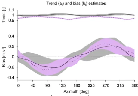
Figure 5.Error estimates of radial wind component for Mode-S EHS- and sodar-based wind vector observations for different az-imuth angles. The black vertical error bar indicates the radial wind error estimate from Mode-S EHS with the radial wind component constructed from the wind vector using the azimuth distribution of the radar data set.
wind vector a radial component is constructed using a pre-scribed azimuth angle. Each error estimate is determined us-ing 10 subsets of the data set, and consequently an tainty of the estimated error can be determined. This uncer-tainty is denoted by the shaded areas in Fig. 5.
ex-Figure 6. Error estimates of radial wind component for Mode-S EHS- and sodar-based wind vector observations for different az-imuth angles. The black vertical error bar indicates the radial wind error estimate from Mode-S EHS with the radial wind component constructed from the wind vector using the azimuth distribution of the radar data set. The shaded area denotes the uncertainty in the estimates, calculated by subdivision of the data set into 10 subsets from which the mean and standard deviation of the estimate are cal-culated.
ploiting (only) three beams. The minimum of the sodar radial wind error is at 0 and 180◦, corresponding to the meridional component, while the maximum error is at 90 and 270◦, cor-responding to the zonal component. For Mode-S EHS the errors in zonal and meridional component are more or less equal; the maxima and minima are attained at approximately 45 and 225◦, and 135 and 315◦respectively.
The trend and bias with respect to the first data set are si-multaneously estimated by the triple-collocation algorithm. Obviously, the bias has no effect on the estimated observa-tion errors; however, it can be informative because it gives information on the mean difference with the truth. The trend displays the scaling of the data set with the truth. Figure 6 shows the trend and bias for the radial wind component of the Mode-S EHS/sodar/NWP data set. The trend of Mode-S EHS is close to 1, indicating that radial wind observations are of the same order. The trend of NWP lies clearly below 1 (0.96±0.02); the radial NWP wind is overestimated when compared to sodar (and Mode-S EHS) radial winds. Note that the trend has a bi-periodic behaviour. The bias shows a dif-ferent signal, both periodic in azimuth with the same phase. Since the signal is equal for both NWP as Mode-S EHS, the origin must lie in the sodar measurement and might be re-lated to the method of observation using three beams or in an azimuth offset. This needs further research.
4.2 Mode-S EHS, radar and sodar wind observation error
Next we discuss the consistency between the estimated Mode-S EHS error from both data sets by inspection of the
Table 3.Mode-S EHS wind component observation error estimate.
Zonal component
level number estimated error
Mode-S EHS (radar/NWP) 913–422 hPa 118 1.23±0.41 Mode-S EHS (sodar/NWP) 0–700 m 2403 1.40±0.10
Meridional component
level number estimated error
Mode-S EHS (radar/NWP) 962–480 hPa 599 1.38±0.20 Mode-S EHS (sodar/NWP) 0–700 m 2403 1.45±0.10
zonal and meridional estimates. The radial wind is equal to the zonal component of the wind for an azimuth angle of 90 and 270◦. Similarly, the radial wind for an azimuth of 0 or 180◦ equals the meridional component. By selecting in the Mode-S EHS/radar/NWP data set azimuth angles between 75 and 105◦(and 255 to 285◦) we can make an estimate of the zonal component of the wind error of Mode-S EHS at levels higher than the sodar. The result is shown in Table 3.
These statistics show consistency between both triple-collocation data sets when taking into account the observed uncertainty of the estimates. Due to the small numbers of Mode-S EHS observations satisfying the azimuth angle conditions, the uncertainty for the estimates based on the Mode-S EHS/radar/NWP data set is larger than for the other triple-collocation data set (for the latter all observations can be used obviously). The uncertainty range of the Mode-S EHS/radar/NWP estimates overlaps the uncertainty of the Mode-S EHS/sodar/NWP. The Mode-S EHS error is approx-imately 1.4 to 1.5 m s−1near the surface. Note that the zonal Mode-S EHS observations are found at a higher altitude, which, as we will see later, influences the magnitude of the error slightly.
The meridional component statistics, shown also in Ta-ble 3, are obtained by selecting angles smaller than 15◦and larger than 345◦ azimuth, and between 165 and 195◦ az-imuth. The estimate of the observation error is larger than the one for the zonal component, but the difference is of the order of 0.1 m s−1. Again the uncertainty of the Mode-S EHMode-S/radar/NWP observation error is larger than the un-certainty from the other data set, and again there is a clear overlap of the uncertainty intervals.
We now focus on the radial wind component of the Mode-S EHMode-S observation error. The result of the triple collocation for all radial wind component is shown in Fig. 7. The error bar denotes again the spread of the triple-collocation standard deviation estimates by dividing the data sets into 10 subsets and estimating the observation error for each subset.
Figure 7.Mode-S EHS radial wind error estimates from the two triple-collocation data sets with respect to altitude. Error bar indi-cates the uncertainty of the error estimates based on error estimates determined from 10 subsets. The size of the data sets is denoted by the numbers on the right.
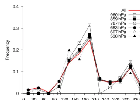
from levels higher than 600 hPa the estimated error is slightly below 1.5 m s−1. The higher levels deviate from 1.5 m s−1, which is related to the distribution of the azimuth angles used to estimate the Mode-S EHS observation error, as can be seen in Fig. 8, where the azimuth distribution is shown in bins of 30◦for the different altitude bins. It is clear from this figure that the two highest estimates (higher than 600 hPa in Fig. 7, the triangles in Fig. 8) have a clear different signature in az-imuth distribution than the lower four estimates. Because the azimuth distributions differ substantially, the reconstructed radial wind data set of the highest levels is not consistent with that of the lowest levels. The distribution of the azimuth angles will influence the magnitude of the observation error estimate (see Fig. 5). In order to have a better comparison between error estimates at different levels, a resampling of the data sets is performed, such that the azimuth distribution for each level matches the azimuth distribution of the whole data set. We used the distribution in 30◦bins as a reference.
Figure 9 shows the resampled distributions. When two or more observed azimuth values are present in the original bin, the resampled bin is filled by randomly sampling (with re-placement) from this bin until the number found is exactly equal to that of the reference bin. Note that when a bin con-tains none or only one azimuth value this bin is skipped. When this occurs, it will influence the number data points in the other bins, because the total number of data points of all bins is kept constant. The consequence is that the az-imuthal distributions will differ from the reference distribu-tion, as can be seen in Fig. 9 for the azimuth distribution of the lowest level (960 hPa, open square) and the highest level (538 hPa, solid triangle). All other new azimuth distributions match the reference very well (Fig. 9).
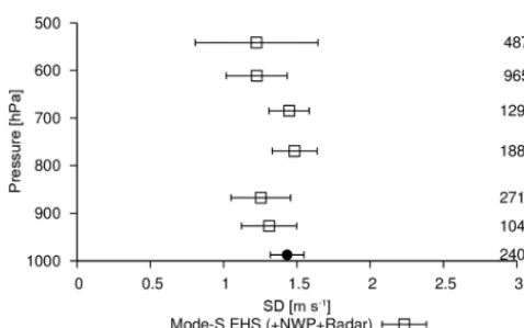
The resulting estimates of Mode-S EHS observation error after resampling are shown in Fig. 10. Again, each data set
Figure 8.Azimuthal distribution of the data sets used to estimate the Mode-S EHS observation error for different altitudes; in red is the azimuth distribution of the complete data set. Azimuth bin is set to 30◦.
Figure 9.Azimuthal distribution of the resampled data sets. Az-imuth bin is set to 30◦.
is subdivided into 10 subsets, which are subsequently used to estimate the uncertainty of the observation error estimate using triple collocation. In general the estimates are slightly smaller than without resampling, while the estimate uncer-tainty is slightly larger, especially for the highest level. The overall increase in uncertainty is related to oversampling of the data set. For example, the increase of uncertainty ob-served for the top level is due to the relatively small num-ber of data points in the altitude bin for this level. It ap-pears that the observation error decreases with altitude above 800 hPa. The numbers used in the triple-collocation increase also slightly because of the resampling, which selects multi-ple data points from an undersammulti-pled (original) bin.
split-Table 4.Trend and bias for resampled radial wind.
Altitude Number aEHS[–] bEHS[m s−1] aNWP[–] bNWP[m s−1]
Radar 541 hPa 487 1.01±0.03 −0.06±0.19 1.02±0.05 0.30±0.67 611 hPa 965 1.00±0.03 0.37±0.25 0.97±0.05 0.25±0.29 685 hPa 1299 0.97±0.01 −0.12±0.21 0.96±0.02 0.09±0.23 769 hPa 1886 0.97±0.02 0.04±0.28 0.96±0.02 0.16±0.23 867 hPa 2716 1.05±0.03 −0.02±0.13 0.98±0.03 −0.05±0.10 927 hPa 1043 0.99±0.05 0.28±0.24 0.97±0.05 0.39±0.20 Sodar 987 hPa 2406 1.00±0.02 0.20±0.18 0.97±0.02 −0.09±0.10
Figure 10.Mode-S EHS radial wind error estimates from the two triple-collocation data sets with respect to altitude. The Mode-S EHS/radar/NWP data set has been resampled to have similar az-imuth distributions. Error bar indicates the uncertainty of the error estimates based on error estimates determined from 10 subsets. The size of the data sets is denoted by the numbers on the right.
ting the data set into 10 subsets. The bias is between −0.1 and 0.4 m s−1with an uncertainty of around 0.2 m s−1. The trend in NWP is smaller than 1, apart from the highest level. The bias is in general positive between 0 and 0.4 m s−1with an uncertainty of around 0.2 m s−1 (again except the high-est level). These numbers are in agreement with the previous trend and bias estimates presented in Fig. 6.
5 Conclusions and outlook
In this study we applied the triple-collocation technique to estimate the Mode-S EHS observation error. We used two triple data sets consisting of Mode-S EHS/sodar and NWP, and Mode-S EHS, radar, and NWP. Using the first data set an estimate of the two horizontal wind vector components was found for observations with an altitude of at most 700 m. The estimated observation error for the wind components was around 1.40 m s−1for the zonal component of the wind and 1.45 m s−1 for the meridional component of the wind. The
uncertainty of these estimates is 0.1 m s−1. The second data set is used to estimate the Mode-S EHS observation along the line of sight of a radar beam. Using this data set, knowledge was gained on the vertical behaviour of the observation error. It turns out the radial wind observation error is not constant with azimuth angle but that the Mode-S EHS observation er-rors of the zonal and meridional component are more or less equal to each other and to the Mode-S EHS observation error constructed using the actual azimuth angle distribution.
The observation error of Mode-S EHS wind vector pro-jected on the radial component has some dependence on alti-tude. The projection is performed using the distribution of the azimuth as observed in the Mode-S EHS/radar/NWP data set. It appears that, after resampling, from the surface to 800 hPa the observation error is between 1.2 and 1.4 m s−1, while from 800 to 500 hPa the error decreases from approximately 1.5 to 1.1 m s−1. However, the uncertainty of the observation error estimate increases with increasing altitude.
In many previous studies to assess the accuracy of aircraft wind observations, a second observing system was used. This implies that, when looking at the statistics of the differences, the error estimates contain errors from both systems and are in fact (at least) a factor of
√
2 larger than the real error (in case we know the “truth”).
The study at hand uses data over a period of 9 months. A longer period would be preferable, but the overlap of avail-ability of Mode-S EHS and a consistent HARMONIE data set was limited to only 9 months. It is anticipated in future research to investigate seasonal effects.
Acknowledgements. EUROCONTROL Maastricht Upper Area Control Centre (MUAC) is kindly acknowledged for the provision of the ASTERIX CAT048 data.
Edited by: A. Stoffelen
Reviewed by: two anonymous referees
References
Benjamin, S. G., Schwartz, B. E., and Cole, R. E.: Accuracy of ACARS Wind and Temperature Observations Deter-mined by Collocation, Weather Forecast., 14, 1032–1038, doi:10.1175/1520-0434(1999)014<1032:AOAWAT>2.0.CO;2, 1999.
Brousseau, P., Berre, L., Bouttier, F., and Desroziers, G.: Background-error covariances for a convective-scale data-assimilation system: AROME–France 3D-Var, Q. J. Roy. Meteor. Soc., 137, 409–422, doi:10.1002/qj.750, 2011.
de Haan, S.: High-resolution wind and temperature observations from aircraft tracked by Mode-S air traffic control radar, J. Geo-phys. Res., 116, D10111, doi:10.1029/2010JD015264, 2011. de Haan, S.: An improved correction method for high quality wind
and temperature observations derived from Mode-S EHS, Tech. Rep. TR338, KNMI, 2013.
Draper, C., Reichle, R., de Jeu, R., Naeimi, V., Parinussa, R., and Wagner, W.: Estimating root mean square errors in remotely sensed soil moisture over continental scale domains, Remote Sens. Environ., 137, 288–298, 2013.
Drüe, C., Frey, W., Hoff, A., and Hauf, T.: Aircraft type-specific errors in AMDAR weather reports from commercial aircraft, Q. J. Roy. Met. Soc., 134, 229–239, 2007.
Drüe, C., Hauf, T., and Hoff, A.: Comparison of Boundary-Layer Profiles and Layer Detection by AMDAR and WTR/RASS at Frankfurt Airport, Bound.-Lay. Meteorol., 135, 407–432, 2010.
Houchi, K., Stoffelen, A., Marseille, G. J., and De Kloe, J.: Com-parison of wind and wind shear climatologies derived from high-resolution radiosondes and the ECMWF model, J. Geophys. Res.-Atmos., 115, D22123, doi:10.1029/2009JD013196, 2010. Nash, J., Smout, R., Oakley, T., Pathack, B., and Kurnosenko, S.:
WMO intercomparison of high quality radiosonde systems, Va-coas, Mauritius, 2–25 February 2005, WMO Report, available from CIMO, 2005.
Painting, J. D.: WMO AMDAR Reference Manual, WMO-no.958, WMO, Geneva, available at: http://www.wmo.int (last access: 4 August 2016), 2003.
Roebeling, R., Wolters, E., Meirink, J., and Leijnse, H.: Triple col-location of summer precipitation retrievals from SEVIRI over Europe with gridded rain gauge and weather radar data, J. Hy-drometeorol., 13, 1552–1566, 2012.
Seity, Y., Brousseau, P., Malardel, S., Hello, G., Bénard, P., Bouttier, F., Lac, C., and Masson, V.: The AROME-France Convective-Scale Operational Model, Mon. Weather Rev., 139, 976–991, doi:10.1175/2010MWR3425.1, 2011.
Stoffelen, A.: Toward the true near-surface wind speed: Error mod-eling and calibration using triple collocation, J. Geophys. Res.-Oceans, 103, 7755–7766, 1998.
Stone, E. K. and Kitchen, M.: Introducing an approach for ex-tracting temperature from aircraft GNSS and pressure alti-tude reports in ADS-B messages, J. Atmos. Ocean. Technol., doi:10.1175/JTECH-D-14-00192.1, April 2015.
Stone, E. K. and Pearce, G.: An operational network of Mode-S re-ceivers for aircraft derived meteorological data, J. Atmos. Ocean. Tech., doi:10.1175/JTECH-D-15-0184.1, Aril 2016.