www.atmos-meas-tech.net/9/3837/2016/ doi:10.5194/amt-9-3837-2016
© Author(s) 2016. CC Attribution 3.0 License.
Close-range radar rainfall estimation and error analysis
C. Z. van de Beek1,4, H. Leijnse2, P. Hazenberg3, and R. Uijlenhoet4
1MeteoGroup, Wageningen, the Netherlands
2Royal Netherlands Meteorological Institute, De Bilt, the Netherlands 3Atmospheric Sciences Department, University of Arizona, Tucson, AZ, USA
4Hydrology and Quantitative Water Management Group, Wageningen University, the Netherlands
Correspondence to:C. Z. van de Beek ([email protected])
Received: 9 March 2016 – Published in Atmos. Meas. Tech. Discuss.: 16 March 2016 Revised: 17 July 2016 – Accepted: 18 July 2016 – Published: 18 August 2016
Abstract. Quantitative precipitation estimation (QPE)
us-ing ground-based weather radar is affected by many sources of error. The most important of these are (1) radar calibra-tion, (2) ground clutter, (3) wet-radome attenuacalibra-tion, (4) rain-induced attenuation, (5) vertical variability in rain drop size distribution (DSD), (6) non-uniform beam filling and (7) variations in DSD. This study presents an attempt to sep-arate and quantify these sources of error in flat terrain very close to the radar (1–2 km), where (4), (5) and (6) only play a minor role. Other important errors exist, like beam block-age, WLAN interferences and hail contamination and are briefly mentioned, but not considered in the analysis. A 3-day rainfall event (25–27 August 2010) that produced more than 50 mm of precipitation in De Bilt, the Netherlands, is analyzed using radar, rain gauge and disdrometer data.
Without any correction, it is found that the radar severely underestimates the total rain amount (by more than 50 %). The calibration of the radar receiver is operationally mon-itored by analyzing the received power from the sun. This turns out to cause a 1 dB underestimation. The operational clutter filter applied by KNMI is found to incorrectly iden-tify precipitation as clutter, especially at near-zero Doppler velocities. An alternative simple clutter removal scheme us-ing a clear sky clutter map improves the rainfall estimation slightly. To investigate the effect of wet-radome attenuation, stable returns from buildings close to the radar are analyzed. It is shown that this may have caused an underestimation of up to 4 dB. Finally, a disdrometer is used to derive event and intra-event specificZ–Rrelations due to variations in the ob-served DSDs. Such variations may result in errors when ap-plying the operational Marshall–PalmerZ–Rrelation.
Correcting for all of these effects has a large positive im-pact on the radar-derived precipitation estimates and yields a good match between radar QPE and gauge measurements, with a difference of 5–8 %. This shows the potential of radar as a tool for rainfall estimation, especially at close ranges, but also underlines the importance of applying radar correc-tion methods as individual errors can have a large detrimental impact on the QPE performance of the radar.
1 Introduction
Rainfall is known to be highly variable, both in time and space. Traditional measurements by single rain gauges or networks only provide accurate information of the rainfall at their locations. While interpolation of these data is possible, the spatial information is often too sparse for accurate mete-orological and hydrological applications (Berne et al., 2004; van de Beek et al., 2011a, b). Furthermore, rain gauges are often seen as “ground truth”, but these instruments also suf-fer from errors (Marsalek, 1981; Sevruk and Nespor, 1998; Habib et al., 2001; Ciach, 2003).
rate from the measured reflectivity aloft due to uncertainties in the rain drop size distribution (DSD) (Uijlenhoet et al., 2003), the impact of wind drift and differences in instrumen-tal characteristics (i.e., radar beam volume vs. point-based rain gauge). These variations in the error sources have been studied and described extensively in the past (e.g., Zawadzki, 1984; Hazenberg et al., 2011a, 2014). Polarimetric radars of-fer new variables that allow greater insight in precipitation and new ways to deal with these error sources, but are not considered in this paper (Bringi and Chandrasekar, 2001).
Clutter results from the main beam or side lobes (partially) reflecting off the terrain or atmospheric objects (e.g., build-ings or trees, airplanes, insects and birds). Close to the radar, ground clutter from objects can lead to overestimation of rainfall reflectivities. Another source of clutter results from atmospheric conditions bending the emitted radar beam to-wards the surface (i.e., anomalous propagation (“anaprop”)). This source of clutter can be highly variable in time, but its overall effect is generally limited. In the past many clutter correction schemes have been developed that reduce the im-pact of clutter with varying degrees of success (e.g., Steiner and Smith, 2002; Holleman and Beekhuis, 2005; Berenguer et al., 2005).
Attenuation of the transmitted signal during a rainfall event can lead to strong underestimation of the rain rate. The amount of attenuation along the path of the transmitted sig-nal is strongly dependent on the rain rate as well as on the transmitted wavelength. X-band radars are relatively inex-pensive and easy to install, but suffer quite strongly from at-tenuation (e.g., van de Beek et al., 2010). Radars operating at longer wavelengths, like C-band and S-band radars, suffer less from attenuation. However, during intense precipitation events, C-band radar rainfall retrievals also tend to underes-timate precipitation rate (e.g., Delrieu et al., 1991; Bouilloud et al., 2009). Correction for rain-induced attenuation was first proposed by Hitschfeld and Bordan (1954). Since then, other schemes have been developed that use a path-integrated at-tenuation constraint (e.g., Bringi et al., 1990; Marzoug and Amayenc, 1994; Delrieu et al., 1997; Testud et al., 2000; Ui-jlenhoet and Berne, 2008). Even though this study is based on a single-polarization radar, it is worth noting that the differentiphase measurements from polarimetric radars al-low new methods (e.g., Gorgucci and Chandrasekar, 2005). Another source of attenuation is caused by precipitation on the radar radome, resulting in a liquid film of water. This film attenuates the signal and its effect becomes more pronounced during stronger precipitation intensities. Wet radome attenu-ation is highly dependent on the wind direction and the state of the radome, as the attenuation depends on whether a film of water can form on the radome (Germann, 1999; Kurri and Huuskonen, 2008).
Vertical variations in precipitation as observed with radar give rise to the so-called vertical profile of reflectivity (VPR). The VPR has an important impact on the measurement char-acteristics of the radar, even though close to the surface, the
role of the VPR tends to be limited. For stratiform precipita-tion, the melting of snowflakes and ice crystals aloft results in relatively large droplets. Within this melting layer region, the returned radar signal intensifies (bright band), leading to an overestimation of the precipitation intensity, while mea-surements above the melting layer typically lead to an un-derestimation (e.g., Andrieu et al., 1995; Vignal et al., 2000; Delrieu et al., 2009; Hazenberg et al., 2013).
Non-uniform beam filling can also cause significant errors. This effect of course depends on the size of the radar mea-surement volume and the spatial heterogeneity of the fall. Because the relation between radar reflectivity and rain-fall intensity is nonlinear and not unique (depending on the DSD), spatial rainfall variability within the radar measure-ment volume can cause errors (Fabry et al., 1992; Berne and Uijlenhoet, 2005; Sassi et al., 2014). The DSD also directly influences the relation between the radar reflectivity and spe-cific attenuation. In case rain-induced attenuation is not cor-rected for, the radar product is prone to result in erroneous rainfall estimates (Gosset and Zawadzki, 2001).
The conversion from measured reflectivity values to rain rates at ground level can be quite challenging as rain is highly variable in terms of its DSD (e.g., Uijlenhoet et al., 2003; Yuter et al., 2006). In general, the reflectivity value (Z) is converted into a rainfall rate (R) using a power-law relation:
Z=aRb. (1)
To date, the Marshall–Palmer (M–P) equation (Marshall et al., 1955) withZ=200R1.6 is the most commonly used
Z–Rrelationship and is generally assumed to be representa-tive of stratiform precipitation. It should be noted that other
Z–Rrelations have been derived as well, more suitable dur-ing different types of precipitation and for other locations (e.g., Battan, 1973; Fulton et al., 1998; Uijlenhoet, 2001; Ui-jlenhoet and Berne, 2008). Estimates of the DSD can be ob-tained by surface disdrometers, from which bothZandRcan be inferred. Based on these estimates, it then becomes possi-ble to infer the actualZ–Rrelationship for the event of study at the location of the instrument (e.g., Löffler-Mang and Joss, 2000; Berne and Uijlenhoet, 2005; Hazenberg et al., 2011b). However, the benefit of applying disdrometer observations for weather radar rainfall correction application is still un-certain, as their point-based character might not be represen-tative of the larger scale precipitation system aloft. Hazen-berg et al. (2014) showed that using a disdrometer to deter-mine the actualZ–R relation did lead to improved results for convective precipitation. At the same time, making use of disdrometer observations for the Netherlands was shown to lead to improved precipitation estimates for widespread stratiform precipitation (Hazenberg et al., 2016)
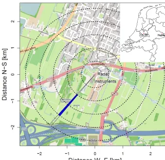
Figure 1.Locations of the rain gauge, disdrometer and radar at De Bilt with 0.5 km range rings around the radar (dashed lines). The blue section is the 1–2 km radar bin that is used in this study. The inset in the upper right corner shows the locations of radar and instruments at De Bilt and at Hupsel, which is the location of maximum rainfall measured during the event studied. Data by OpenStreetMap.org contributors under CC BY-SA 2.0 license.
phenomenon whose effects over medium to long accumu-lation intervals might not be detrimental, even if not cor-rected. Beam blockage, despite quantifiable and correctable to a given extent, affects the adopted scan strategy and the height of measurements above ground.
WLAN interference is increasingly becoming an issue for weather radar measurements, but is not considered in this pa-per. A recent publication on this topic is, e.g., Saltikoff et al. (2015).
Hail can also heavily affect radar observations in terms of both scattering and absorption enhancement. For C-band radar, melting hail can be responsible for attenuation en-hancement that can lead to signal extinction.
This paper studies the possibilities of quantitative precip-itation estimation (QPE) at close ranges (1–2 km) for a C-band weather radar operated by the Royal Netherlands Mete-orological Institute (KNMI) in the center of the Netherlands. At these distances, the effects of VPR, rain-induced attenua-tion and non-uniform beam filling are limited. Their impact was therefore ignored in this work. Section 2 describes the instruments and the data used in this study, which are the
same as used by Hazenberg et al. (2014). Section 3 describes the rain event that is analyzed. On Sect. 4 the reflectivity cor-rection methods and their effects are discussed, together with a verification. Finally, Sect. 5 contains conclusions and rec-ommendations.
2 Instruments and data
The employed rain gauge is an automatic gauge with a surface area of 400±5 cm2 installed in a pit (Wauben, 2004, 2006). The height of a float in the reservoir of the gauge is measured every 12 s with a resolution of 0.001 mm. The gauge can report the precipitation intensity in steps of 0.006 mm h−1. The rain is accumulated and stored at 10 min intervals, using guidelines set by Sevruk and Zahlavova (1994) and WMO (1996).
The disdrometer is a first-generation OTT Parsivel®. The Parsivel®measures the size and velocity of droplets by the extinction caused by droplets passing through a sheet of light with a surface area of around 50 cm2. It can measure par-ticles from 0.2 to 25 mm diameter with velocities between 0.2 and 20 m s−1. The beam between transmitter and receiver has been oriented perpendicular to the prevailing southwest-erly wind direction in the Netherlands. The data from the disdrometer are logged every minute (de Haij and Wauben, 2010). The first-generation Parsivel®disdrometer is known to have some issues (Thurai et al., 2011; Tokay et al., 2013). Most notable is the overestimation that occurs for higher rainfall intensities and large raindrops. Tokay et al. (2013) note that the Parsivel®starts to overestimate the number of drops larger than 2.44 mm diameter when intensities exceed 2.5 mm h−1and the drop concentrations exceed 400 min−1. The number of drops in this diameter class (i.e., larger than 2.44 mm) is limited throughout the event presented below, so the effect is expected to be minor.
The radar operated by KNMI is a Doppler C-band radar from SELEX-SI (Meteor AC360). It is located at 52.108◦N, 5.178◦E on top of a tower at 44 m above sea level. It operates at 5.6 GHz (wavelength of 5.3 cm). The radar performs a full 14-elevation volume scan every 5 min. The resolution is 1◦ in azimuth and 1 km in range. For details about the radar and the scan schedule, see Beekhuis and Holleman (2008). For this study we use the first distance bin between 1 and 2 km from the radar at an azimuth of 230◦(see Fig. 1) of the 0.8◦ elevation scan. The analyzed data are from a range in the far field of the radar. The T/R limiter might cause some tenths of a decibel additional attenuation at the close range considered. The limited effect is confirmed, however, as the final rainfall estimates are seen to correspond well with disdrometer and rain gauge measurements (Beekhuis and Leijnse, 2012).
3 Description of the rain event
Between 25 and 27 August 2010, a narrow band of low pres-sure passed over the Netherlands from the direction of the English Channel towards southern Denmark, between high pressure zones over southern Europe and Scotland. During 26 August, the triple point remained near the southern coast of the Netherlands for most of the day with the warm front moving very slowly northward. This caused large tempera-ture differences in the Netherlands between the north, with cold air, and the south, with warmer air behind the warm
Figure 2.Synoptic situation for 26 August 2010, 12:00 UTC.
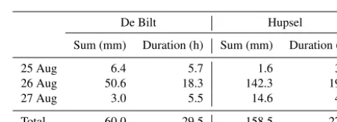
Table 1.Daily precipitation sum and duration on 25–27 August.
De Bilt Hupsel
Sum (mm) Duration (h) Sum (mm) Duration (h)
25 Aug 6.4 5.7 1.6 3.0
26 Aug 50.6 18.3 142.3 19.5
27 Aug 3.0 5.5 14.6 4.5
Total 60.0 29.5 158.5 27.0
front. During the afternoon of the 26th the low pressure zone began moving eastwards, leading to calmer weather (see Fig. 2).
During the passage of these low-pressure areas, a mesoscale convective system containing large fields of alter-nately stratiform and convective precipitation passed over the Netherlands. This led to both large precipitation amounts and long durations for most of the Netherlands. Table 1 illustrates the amounts and durations for De Bilt, where the radar and instruments are located, and for Hupsel, located in the east of the Netherlands. At Hupsel, an extremely large amount of precipitation of nearly 160 mm within 24 h was measured (return period>1000 years) for this event (see Brauer et al., 2011; Hazenberg et al., 2014). At the location of the radar in De Bilt, which is the focus of this study, the total precipita-tion accumulaprecipita-tion was less, although still considerable, with 50.6 mm over a period of 18.3 h of continuous rain (return period 5–10 years; see Overeem et al., 2008, 2009).
Wed Thu Fri Sat
0
5
10
15
20
25 Gauge
Radar
R
a
in
ra
te
[
m
m
h
]
−
1
1 2 3 4 5 6 7 8
Wed Thu Fri Sat
0
10
20
30
40
50
60
70 Radar
Parsivel Gauge
Cum
ulativ
e r
ain [mm]
Time
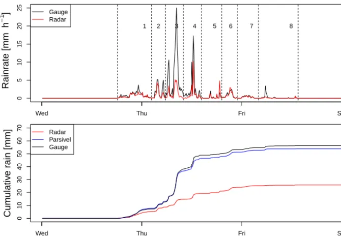
Figure 3.Top panel: time series of the rain event, with the rain rate from the rain gauge in black, and in red, the rain rate derived from the
radar reflectivity using the Marshall–PalmerZ–Rrelation (M–P). The vertical dashed lines divide the event into eight different episodes.
Bottom panel: cumulative sum of rainfall from the three instruments before any correction of the radar and using the M–P relation.
0 1 2 3 4 5
20:00 2:00 8:00 14:00 20:00 2:00 08:00 14:00
1 2 3 4 5 6 7 8
Drop diameter (mm)
Date
2010−08−25 2010−08−27
1 2−5 6−10 11−20 21−30 31−40 41−50 51−75 76−100 101−125 126−150 151−200 200−400 >400
Drop counts
Figure 4.DSD during the rain event. The black dashed lines
illus-trate the identified rain episodes of the event.
Fig. 3), and a second one containing heavier rainfall rates up to 25 mm h−1(episode 3 in Fig. 3). This period also gave rise to the largest number of raindrops measured by the Parsivel® disdrometer (see Fig. 4). The large peak in episode 4 was the edge of an active squall line that began to form south of the radar and was advected eastwards, which caused large precipitation sums near Hupsel (Brauer et al., 2011). For episodes 5–8, rain intensities decreased within the trailing stratiform part of the squall line, resulting in sporadic rain-fall observed close to the radar. The total accumulations are shown in the bottom panel of Fig. 3. The two disdrometers and the gauge are closely related, but the radar clearly under-estimates rainfall accumulations.
4 Methodology and results
As explained in the introduction, various error sources af-fect rainfall measurements by weather radar. Since this work focuses on the performance of the weather radar at close ranges, it was decided not to focus on the impact of rain-induced attenuation and VPR, as at close ranges these are ex-pected to be negligible. Therefore, the current section specif-ically focuses on the effects of correcting for calibration, ground clutter and wet-radome attenuation. Furthermore, this section also presents the impact of accounting for DSD vari-ations as inferred from disdrometer observvari-ations.
4.1 Calibration
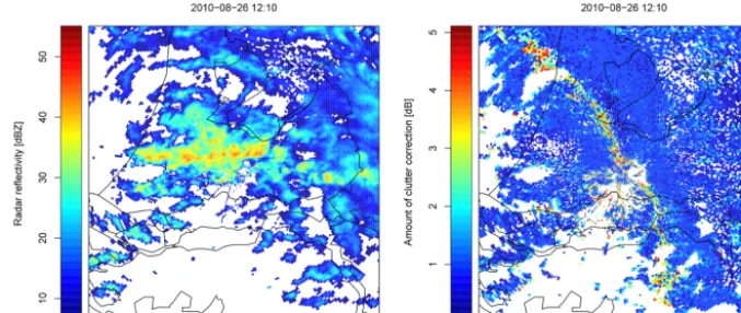
Figure 5.Radar reflectivity (left panel) and amount of clutter corrected by the Doppler notch filter (right panel) for the most intense rainfall
peak of episode 4 on 26 August 2010 at 12:10 UTC. Images shown are for the 0.8◦elevation scan.
for this error source, a value of 1 dB was added to the ob-served radar reflectivity values.
4.2 Clutter correction
The operational ground clutter correction algorithm uses a time-domain Doppler notch filter. A drawback of this auto-matic procedure is that it incorrectly identifies some precipi-tation as clutter (e.g., Hubbert et al., 2009), leading to an un-derestimation of rainfall intensities as measured by the radar. An example is clearly shown in Fig. 5, where images of both the radar reflectivity factor and the amount of clutter correc-tion are shown. The zero-isoDop, the region where the veloc-ity is perpendicular to the radar and therefore zero, is clearly visible in the right-hand panel of this image, and the amount of filtering in such areas can be as high as 3–4 dB. For other areas, the amount of incorrect identification of precipitation as ground clutter is limited, although its effect can still be significant, on the order of 1–2 dB (i.e., a factor of 1.15–1.33 in terms of rainfall intensity given the Marshall–PalmerZ–R
relation).
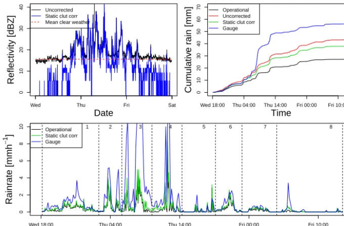
As an alternative procedure to correct for the impact of ground clutter, use was made of a dry weather clutter map technique, consisting of the average dry weather reflectiv-ity value. To correct for the impact of ground clutter during the precipitation event, this map is subtracted from the ob-served reflectivity values. Normally such a technique is ap-plied to every pixel within the radar map, but for this study it has only been applied to the bin of interest. A main underly-ing assumption of makunderly-ing use of a static dry weather clutter map is that the clutter reflectivity does not change during rain (e.g., because objects become wet). This method (also called a clutter map) will not remove all clutter; however, it identi-fies less precipitation as clutter compared to a Doppler filter. Figure 6 illustrates the effect of the operational clutter re-moval scheme and the use of the static dry weather clutter map. In the top-left panel, the raw uncorrected reflectivity values are shown in black. It can be observed that the average
background reflectivity values during clear sky situations are around 15.6 dBZ (dashed red line). Subtraction of the mean value ofZ (mm6m−3) (i.e., not dBZ) from the uncorrected reflectivity results in the simple static clutter removal (blue line). This has the greatest impact for low reflectivities, with no or very little rain.
In the top-right panel of Fig. 6, the cumulative rainfall sums are shown for both rain gauge and radar rainfall (us-ing the M–P relation) data. Radar accumulations are shown without clutter correction, and after applying either an oper-ational Doppler scheme or the static dry-weather clutter cor-rection method. Note that these results are obtained after ap-plying 1 dB calibration correction. Results show that the un-corrected radar reflectivities produce the largest rainfall accu-mulations, as results are overestimated due to the identifica-tion of ground clutter as precipitaidentifica-tion. Of the two clutter cor-rection schemes, applying the operational Doppler scheme results in the largest reduction of precipitation, whereas the static scheme is more conservative. As explained before, it is anticipated that the operational Doppler scheme incorrectly identifies some precipitation as ground clutter and as such results in the lowest precipitation accumulations. Therefore, in the remainder of the paper, use is made of the static-clutter correction scheme.
pos-Wed Thu Fri Sat
0
10
20
30
40
Reflectivity [dBZ]
Date Uncorrected
Static clut corr Mean clear weather
Wed 18:00 Thu 04:00 Thu 14:00 Fri 00:00 Fri 10:00
0
10
20
30
40
50
60
70 Operational Uncorrected Static clut corr Gauge
Cum
ulativ
e r
ain [mm]
Time
Wed 18:00 Thu 04:00 Thu 14:00 Fri 00:00 Fri 10:00
0
2
4
6
8
10 Operational Static clut corr Gauge
Rainr
ate [
m
m
h
−
1 ]
Time
1 2 3 4 5 6 7 8
Figure 6.Top-left panel: reflectivity of the studied range bin between 1 and 2 km from the radar of the uncorrected reflectivity (black) and
the static-clutter-corrected reflectivity (blue). Here the red dashed line is the average reflectivity when there is no rain. Top right panel: the cumulative rain sums for the rain gauge (blue) and the Doppler clutter-corrected reflectivity (black), together with the uncorrected (red) and
the static-clutter-corrected reflectivity (green) using the Marshall–PalmerZ–Rrelation with 1 dB added to compensate for calibration errors.
Bottom panel: time series of the rain gauge, Doppler clutter-corrected and the static-clutter-corrected rain rates.
sible cause might be that the studied range bin lies further south than the other instruments, located at the measurement field of KNMI, and most of the strongest precipitation passed just south of the radar, especially during the formation of the squall line at the end of the rain event.
4.3 Wet radome attenuation
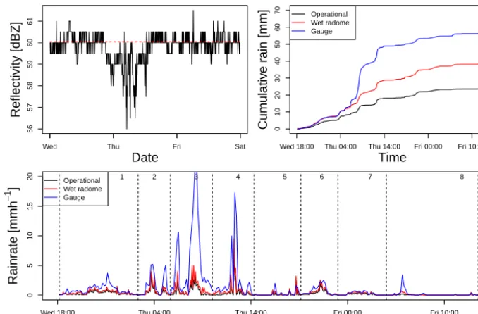
Since for the current event, precipitation with considerable intensities was observed at the location of the radar for a large period of time, it is highly likely that the resulting formation of a thin layer of water on top of the radome caused signif-icant attenuation of the signal. The effect of the wet radome needs to be corrected and is achieved by using a strong clut-ter pixel observed close to the radar, caused by a tall building. Due to its close proximity to the radar (only 3 km away), it is assumed that the impact of the rain-induced attenuation is negligible. We relate a decrease in the measured reflectivity value of this static clutter pixel during a precipitation event to the amount of attenuation caused by the wetting of the radome. While the wetting of the clutter object and precipi-tation at the clutter location may also influence the measured reflectivity, these factors are assumed to be much smaller than the effect of the wetting of the radome.
Figure 7 presents the impact of wet-radome attenuation on the measurement capabilities of the radar. The top-left panel shows the measured reflectivity from the clutter pixel at a range between 3 and 4 km from the radar. The dashed red line presents the average reflectivity during dry periods. The
reflectivity can be seen to fluctuate by about 0.5 dB around this mean value; however a larger drop in measured reflec-tivity values can be observed at the onset of the event in the late afternoon on 25 August. The difference between the av-erage dry and observed reflectivity values is assumed to rep-resent the impact of wet-radome attenuation, which reaches its greatest value during the peak of very heavy rainfall. Af-ter having corrected for calibration error and clutAf-ter, the im-pact of wet-radome attenuation correction is shown in the top-right panel of Fig. 7. As expected, the correction of the attenuated radar reflectivity results in a larger estimated rain rate, closer to that of the rain gauge.
4.4 Z–Rrelations
Wed Thu Fri Sat 56 57 58 59 60 61 Reflectivity [dBZ] Date
Wed 18:00 Thu 04:00 Thu 14:00 Fri 00:00 Fri 10:00
0 10 20 30 40 50 60 70 Operational Wet radome Gauge Cum ulativ e r ain [mm] Time
Wed 18:00 Thu 04:00 Thu 14:00 Fri 00:00 Fri 10:00
0 5 10 15 20 Operational Wet radome Gauge Rainr ate [ m m h − 1 ] Time
1 2 3 4 5 6 7 8
Figure 7.Top-left panel: reflectivity of a strongly reflective clutter pixel near the radar. Here the red dashed line is the average reflectivity
when there is no rain. Top right panel: the cumulative rain for the rain gauge (blue), the Doppler clutter-corrected (black) and the
wet-radome-attenuation-corrected rain rate using the Marshall–PalmerZ–Rrelation using the static-clutter- and calibration-corrected data (red). Bottom
panel: time series of the rain gauge, KNMI (Doppler filter) clutter-corrected and the wet-radome-attenuation-corrected rain rates.
● ● ● ●● ● ● ●●● ●●●●● ● ● ●●●●●●● ●●●●●●●●●●●●●● ●●●● ●● ●● ●● ● ● ● ● ●●●● ●● ● ● ● ●● ●●● ● ●●● ●● ● ● ● ● ● ●● ● ● ● ● ● ● ● ● ● ● ● ● ● ● ●●●●●●●●●●●● ● ● ● ● ●● ● ● ● ●●●● ● ● ● ● ● ● ●● ● ● ● ●● ●● ● ● ● ● ● ● ● ● ● ● ● ●●●●●●●●●● ●● ● ● ● ● ● ● ● ● ● ●●●●●●●●● ●●●● ● ●● ● ● ● ● ● ● ● ● ● ● ● ●● ●● ● ● ● ● ● ● ● ● ● ● ● ● ● ● ● ● ● ● ●
0 5000 10 000 15 000 20 000
0 5000 10 000 20 000
Reflectivity
● ● ● ●● ● ● ●●● ●●●●● ● ● ●●●●●●●●●●●●●●●●●●●● ● ●●●● ●● ●● ●● ● ● ● ● ●●●● ● ● ● ● ● ●● ●● ● ● ●●● ● ● ● ● ● ● ● ●●● ● ● ●● ● ● ● ● ● ● ● ● ● ●●●●●●●●●●●● ● ● ● ● ●● ● ● ● ●●●● ● ● ● ● ●● ●● ● ● ● ●● ●● ● ● ● ● ● ● ● ● ● ● ● ●●●●●●● ● ● ● ● ● ● ● ● ● ● ● ● ● ● ●●●●●●●●● ●●●● ● ●● ● ● ● ● ● ● ● ● ● ● ● ●● ●● ● ● ● ● ● ● ● ● ● ● ● ● ● ● ● ● ● ● ● 0 5000 0 5000 Radar [Z] Parsivel [Z] ● ● ● ● ● ● ● ● ● ● ● ● ● ● ● ● ● ● ● ● ● ● ● ● ● ●●● ● ● ● ● ● ● ●● ● ● ● ● ● ● ● ● ● ● ● ● ● ● ● ● ●● ● ● ● ● ● ● ● ● ●● ● ● ● ● ● ● ● ● ● ● ● ● ● ● ● ● ●●● ● ● ● ● ● ● ● ● ● ● ● ● ● ● ● ● ● ● ● ● ● ● ● ● ● ● ● ● ● ● ● ● ● ● ● ● ● ● ● ● ● ● ● ● ●● ● ●●●● ● ● ● ● ● ● ● ●● ● ● ● ● ● ● ● ● ●● ● ● ● ● ● ● ● ● ●● ● ● ● ● ● ● ● ● ● ●● ● ● ● ● ● ● ● ● ● ● ● ● ● ● ● ● ● ● ● ● ● ●10 15 20 25 30 35 40 45
10 15 20 25 30 35 40 45 ● ● ● ● ● ● ● ● ● ● ● ● ● ● ● ●● ● ● ● ● ●●●● ●● ● ● ● ● ● ● ● ●● ● ● ● ● ● ● ● ● ● ● ● ● ● ● ● ● ● ● ● ● ● ● ● ● ● ● ● ●● ● ● ● ● ● ● ● ● ● ● ● ● ● ● ● ● ● ●● ● ● ● ● ● ●● ● ● ● ● ● ● ● ●●● ● ● ● ● ● ● ● ● ● ● ● ●● ● ● ● ● ● ● ● ● ● ● ● ● ● ● ● ● ● ● ● ● ● ● ● ● ● ● ● ● ● ● ● ●● ● ● ● ● ● ● ● ● ● ● ● ● ● ● ● ● ● ● ● ●● ● ● ● ● ● ● ● ● ●● ● ● ● ● ● ● ● ●●● ● ● ● ● ● ● ● ● ● ● ● ● ● ● ● ● ● ● ● ● ● ● ● ● ● ● ●
10 15 20 25 30 35 40 45
10 15 20 25 30 35 40 45 Radar [dBZ] Parsivel [dBZ] ● ● Operational Corrected
Figure 8. Left panel: reflectivity (Z) measured by the radar and
derived from the Parsivel®, where the black circles are the
opera-tionally corrected values and the red circles the fully corrected data described in this paper. Right panel: same as left panel but on a logarithmic scale.
clutter and wet-radome attenuation (see Fig. 7). While this is still below the accumulated rain sum of 56.3 mm for the rain gauge, the net effect is considerable. Since the current precipitation event was highly variable in space and time, the applied M–P relationship is expected not to be suitable as it is representative of stratiform precipitation conditions. Therefore, further improvements in the quality of the rainfall estimates by radar can presumably be obtained using theZ–
Rrelationship inferred from the disdrometer measurements.
4.4.1 Z–Rrelation derivation
Both the radar reflectivityZ(mm6m−3) and the precipitation intensityR(mm h−1) can be expressed as integral variables of the raindrop size distributionN (D)(mm−1m−3), where
Z=
∞ Z
0
D6N (D)dD, (2)
and
R=6π×10−4
∞ Z
0
D3v(D)N (D)dD, (3)
wherev(m s−1) is the terminal raindrop fall velocity. Hence, bothZandRare functions of the DSD.
The relation between radar reflectivity and rainfall inten-sity can be expressed as a power-law function (Battan, 1973):
Z=aRb. (4)
The observations obtained by the Parsivel® disdrometer are analyzed in more detail here, as from the measurement taken by this instrument, joint estimates ofZandR are ob-tained. These observations enable one to study the impact of event- and intra-event-based variations of theZ–R relation different from the M–P relationship.
● ● ● ● ● ● ● ● ● ● ● ● ● ● ● ● ● ● ● ● ● ● ● ● ● ● ● ● ● ● ● ● ● ● ● ● ● ● ● ● ● ● ● ● ● ● ● ● ● ● ● ● ● ● ● ● ● ● ● ● ● ● ● ● ● ● ● ● ● ● ● ● ● ● ● ● ● ● ● ● ● ● ● ● ● ● ● ● ● ● ● ● ● ● ● ● ● ● ● ● ● ● ● ● ● ● ● ● ● ● ● ● ● ● ● ● ● ● ● ● ● ● ● ● ● ● ● ● ● ● ● ● ● ● ● ● ● ● ● ● ● ● ● ● ● ● ● ● ● ● ● ● ● ● ● ● ● ● ● ● ● ●●●●●●●●●●●●●●●●●●●●●●●●●●●●●●●●●●●●●●●●●●●●●●●●●●●●●●●●●●●●●●●●●●●●●●●●●●●●●●●●●●●●●●●●●●●●●●●●●●●●●●●●●●●●●●●●●●●●●●●●●●●●●●●●●●●●●●●●●●●●●●●●●●●●●●●●●●●●●●●●●●●●●●●●●●●●●●●●●●●●●●●●●●●●●●●●●●●●●●●●●●●●●●●●●●●●●●●●●●●●●●●●●●●●●●●●●●●●●●●●●●●●●●●●●●●●●●●●●●●●●●●●●●●●●●●●●●●●●●●●●●●●●●●●●●●●●●●●●●●●●●●●●●●●●●●●●●●●●●●●●●●●●●●●●●●●●●●●●●●●●●●●●●●●●●●●●●●●●●●●●●●●●●●●●●●●●●●●●●●●●●●●●●●●●●●●●●●●●●●●●●●●●●●●●●●●●●●●●●●●●●●●●●●●●●●●●●●●●●●●●●●●●●●●●●●●●●●●●●●●●●●●●●●●●●●●●●●●●●●●●●●●●●●●●●●●●●●●●●●●●●●●●●●●●●●●●●●●●●●●●●●●●●●●●●●●●●●●●●●●●●●●●●●●●●●●●●●●●●●●●●●●●●●●●●●●●●●●●●●●●●●●●●●●●●●●●●●●●●●●●●●●●●●●●●●●●●●●●●●●●●●●●●●●●●●●●●●●●●●●●●●●●●●●●●●●●●●●●●●●●●●●●●●●●●●●●●●●●●●●●●●●●●●●●●●●●●●●●●●●●●●●●●●●●●●●●●●●●●●●●●●●●●●●●●●●●●●●●●●●●●●●●●●●●●●●●●●●●●●●●●●●●●●●●●●●●●●●●●●●●●●●●●●●●●●●●●●●●●●●●●●●●●●●●●●●●●●●●●●●●●●●●●●●●●●●●●●●●●●●●●●●●●●●●●●●●●●●●●●●●●●●●●●●●●●●●●●●●●●●●●●●●●●●●●●●●●●●●●●●●●●●●●●●●●●●●●●●●●●●●●●●●●●●●●●●●●●●●●●●●●●●●●●●●●●●● ● ● ● ● ● ● ● ● ● ● ● ● ● ● ● ● ● ● ● ● ● ● ● ● ● ● ● ●●●●●●●●●●●●●●●●●●●●●●●●●●●●●●●●●●●●●●●● ● ● ● ● ● ● ● ● ● ● ● ● ● ● ● ● ● ● ● ● ● ● ● ● ● ● ● ● ●●●●●●●●●●●●●●●●●●●●●●●●●●●●●●●●●●●●●●●●●●●●●●●● ● ● ● ● ● ● ● ● ● ● ● ● ● ● ● ● ● ● ● ● ● ●●●●●●● ● ● ● ● ● ● ● ● ● ● ● ● ● ● ● ● ● ● ● ● ● ● ● ● ● ● ● ● ● ● ● ● ● ● ● ● ● ● ● ● ● ● ● ● ● ● ● ● ● ●●● ● ● ● ● ● ● ● ● ● ● ● ● ● ● ● ● ● ● ● ● ● ● ● ● ● ● ● ● ● ● ● ● ● ● ● ● ● ● ● ● ● ● ● ● ● ● ● ● ● ● ● ● ● ● ● ● ● ● ● ● ● ● ● ● ● ● ● ● ● ● ● ● ● ● ● ● ● ● ● ● ● ● ● ● ● ● ● ● ● ● ● ● ● ● ● ● ● ● ● ● ● ● ● ● ● ● ● ● ● ● ● ● ●●● ● ● ● ● ● ● ● ● ● ● ● ● ● ● ● ● ● ● ● ● ● ● ● ● ● ● ● ● ● ● ● ● ● ● ● ● ● ● ● ● ● ● ● ● ● ● ● ● ● ● ● ● ● ● ● ● ● ● ● ● ● ● ● ● ● ● ● ● ● ● ● ● ● ● ● ● ● ● ● ● ● ●●● ● ● ● ● ● ● ● ● ● ● ● ● ● ● ● ● ● ● ● ● ● ● ● ● ● ● ●● ● ● ● ● ● ● ● ● ● ● ● ● ● ● ● ● ● ● ● ●● ● ● ● ● ● ● ● ● ● ● ● ● ● ● ● ● ● ● ● ● ● ● ● ● ●● ● ● ● ● ● ● ● ● ● ● ● ● ● ●● ● ● ● ● ● ● ● ● ● ● ● ● ● ● ● ● ● ●●●● ● ● ● ● ● ● ● ● ● ● ● ● ● ● ● ● ● ● ● ● ● ● ● ● ● ● ● ● ● ● ● ● ● ● ● ● ● ●● ● ● ● ● ● ● ● ● ● ● ● ● ● ●●●●● ● ● ● ● ● ● ● ● ●● ●●●● ● ● ● ● ● ● ● ● ● ● ● ● ● ● ● ● ● ● ● ● ● ● ● ● ● ● ● ● ● ● ● ● ● ●● ● ●● ● ● ● ● ● ● ● ● ● ● ● ● ● ● ● ● ● ●● ● ● ● ● ● ● ● ● ● ● ● ● ● ● ● ● ● ● ● ● ● ● ● ● ● ● ● ● ●● ●● ● ● ● ● ● ● ● ● ● ● ● ● ● ● ● ● ● ● ● ● ●
0 5 10 15 20
0
2000
6000
All
alin=188 blin=1.39
anon−lin=164 bnon−lin=1.5
● ● ● ● ● ● ● ● ● ● ● ● ● ● ● ● ● ● ● ● ● ● ● ● ● ● ● ● ● ● ● ● ● ● ● ● ● ● ● ● ● ● ● ● ● ● ● ●●●●●●●●●●●●●●●●●●●●●●●●●●●●●●●●●●●●●●●●●●●●●●●●●●●●●●●●●●●●●●●●●●●●●●●●●●●●●●●●●●●●●●●●●●●●●●●●●●●●●●●●●●●●●●●●●●●●●●●●●●●●●●●●●●●●●●●●●●●●●●●●●●●●●●●●●●●●●●●●●●●●●●●●●●●●●●●●●●●●●●●●●●●●●●●●●●●●●●●●●●●●●●●●●●●●●●●●●●●●●●●●●●●●●●●●●●●●●●●●●●● ● ● ● ● ● ● ● ● ● ● ● ● ● ● ● ●●●●●●●●●●●●●●●●●●●●●●●●●●●●●●●●●●●●●●●●●●●●●●●●●●●●●●●●●●●●● ● ● ● ● ● ● ● ● ● ● ● ● ●● ● ● ● ● ● ● ● ● ● ● ● ● ● ● ● ● ● ● ● ● ● ● ● ●●●●●●●●● ● ● ● ● ● ● ● ● ● ● ● ● ●● ● ● ● ● ● ● ● ● ● ● ● ● ● ● ● ● ●●●●●●●●●●●●●●●●● ● ● ● ● ● ● ● ● ● ● ●● ● ● ●●●●●●●●●●● ●●●
0 5 10 15 20
0
2000
6000
Episode 1
alin=228 blin=1.4
anon−lin=306 bnon−lin=1.1
● ● ● ● ● ● ● ● ● ● ● ● ● ● ● ● ● ● ● ● ● ● ● ● ● ● ● ● ● ● ● ● ● ● ● ● ● ● ● ● ● ● ● ● ● ● ● ● ●●●●●●●●●●●●●●●●●●●●●●●●●●●●●●●●●●●●●●●●●●●●●●●●●●●●●● ● ● ● ● ●● ● ● ● ● ● ●●● ● ● ● ● ● ● ● ● ● ● ● ● ● ● ● ●●● ●● ● ●●● ● ●● ● ● ● ● ● ● ● ● ● ● ● ● ● ● ● ● ● ● ● ● ● ● ● ● ●
0 5 10 15 20
0
2000
6000
Episode 2
alin=227 blin=1.43
anon−lin=100 bnon−lin=2.1
● ● ● ●●●●●●●●●●●●●●●●●●●●●●●●●●●●●●●●●●●●●●●●●●●●●●●●●●●●●●●●●●●●●●●●●●●●●●●●●●●●●●●●●●●●●●●●●●●●●●●●●●●●●●●●●●●●●●●●●●●●●●●●●●●●● ● ● ● ● ●●●●●● ●●●●● ● ● ● ● ● ● ● ● ●●●●●●●●●● ● ● ● ●● ● ● ● ● ● ● ●●●●●●●● ●●● ● ● ● ●● ● ●● ● ● ● ● ● ●●●● ● ● ● ● ● ● ● ● ● ●● ● ● ● ● ● ● ● ● ● ● ● ● ● ● ● ● ● ● ● ● ● ● ● ● ● ● ● ● ● ● ● ● ●● ● ● ● ● ● ● ● ● ● ● ● ● ● ● ● ●
0 5 10 15 20
0
2000
6000
Reflectivity (Z) [
m
m
6m
− 3]
Episode 3
alin=101
blin=1.48 anon−lin=71
bnon−lin=1.7 ● ● ● ● ● ● ● ● ● ● ● ● ● ● ● ● ● ● ● ● ● ●●●●●●●●●●●●●●●●●●●●●●●●●●●●●●●●●●●●●●●●●●●●●●●●●●●●●●●●●●●●●●●●●●●●●●●●●●●●●●●●●●●●●●●●●●●●●●● ● ● ● ● ● ● ● ● ●●● ● ● ● ● ● ● ● ● ● ● ● ●●●●●●●●●●●●●●● ● ● ● ● ● ● ● ● ● ●●●●●●●●●●●●●●●●●●●●●● ●● ● ● ●● ● ●●● ● ●● ● ●●● ● ● ● ● ● ● ●● ● ● ● ● ●● ● ● ● ● ● ● ●
0 5 10 15 20
0
2000
6000
Episode 4
alin=176
blin=1.37 anon−lin=98
bnon−lin=1.6
●●●●●●●●●●●●●●●●●●●●●●●●●●●●●●●●●●●●●●●●●●●●●●●●●●●●●●●●●●●●●●●●●●●●●●●●●●●●●●●●●●●●●●●●●●●●●●●●●●●●●●●●●●● ● ● ● ● ● ●
0 5 10 15 20
0
2000
6000
Episode 5
alin=161
blin=1.38 anon−lin=122
bnon−lin=1.7
● ● ● ● ● ● ● ● ● ● ● ● ● ● ● ● ●●●●●●●●●●●●●●●●●●●●●●●●●●●●●●●●●●●●●●●●●●●●●●●●●●●●●●●●●●●●●●●●●●●●●●●●●●●●●●●●●●●●●●●●●●●●●●●●●●●●●●●●●●●●●●●●●●●●● ● ● ●●● ● ● ● ● ● ● ● ● ● ● ● ●●●● ● ●● ● ● ● ● ● ● ● ●●●● ● ● ●● ● ● ● ● ● ● ● ● ● ●● ● ● ● ● ● ● ● ● ● ● ● ● ●● ● ● ● ● ● ●● ● ● ● ● ●● ● ● ● ● ● ●
0 5 10 15 20
0
2000
6000
Episode 6
alin=282
blin=1.55
anon−lin=245 bnon−lin=2.2
● ● ● ● ● ● ● ● ● ● ● ● ● ● ● ● ● ● ● ● ● ● ● ● ● ● ● ● ● ● ● ● ● ● ● ● ● ● ●●●●●●●●●●●●●●●●●●●●●●●●●●●●●●●●●●●●●●●●●●●●●●●●●●●●●●●●●●●●●●●●●●●●●●●●●●●●●●●●●●●●●●●●●●●●●●●●●●●●●●●●●●●●●●●●●●●●●●●●●●●●●●●●●●●●●●●●●●●●●●●●●●●●●●●●●●●●●●●●●● ●● ●
0 5 10 15 20
0
2000
6000
Rain rate [mmh
−1]
Episode 7
alin=267
blin=1.44
anon−lin=298 bnon−lin=2.6
● ● ● ●●●●●●●●●●●●●●●●●●●●●●●●●●●●●●●●●●●●●●●●●●●●●●●●●●●●●●●●●●●●●●●●●●●●●●●●●●●●●●●●●●●●●●●●●●●●●●●●●●●●●●●●●●●●●●●●●●●●●●●●●●●●●●●●●●●●●●●●●●●●●●●●●●●●●●●●●●●●●● ●●●●
● ●●
0 5 10 15 20
0
2000
6000
Episode 8
alin=93
blin=1.26
anon−lin=43 bnon−lin=1.8
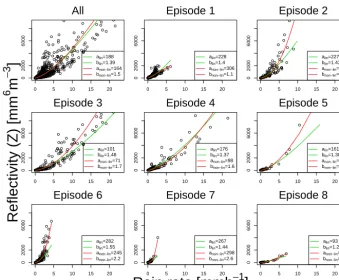
Figure 9.Z–Rrelations derived from the 1 min data of the Parsivel®for the different rainfall episodes distinguished in Fig. 3 using linear
regression on the logarithmic values (green curves) and nonlinear regression (red curves).
are presented. Multiple methods have been presented to de-rive theZ–Rrelationship (Morin et al., 2003; Chapon et al., 2008; Hazenberg et al., 2011b). The simplest approach is to apply a least squares linear regression procedure on the logarithms of Z and R. However, this approach tends to give more weight to smaller rainfall intensities. Therefore as a second approach, in the current work, a nonlinear least squares fitting procedure was also applied and the results are presented in Table 2. From Fig. 9 it can be observed that the applied fitting technique has a large impact on the estimated values of the prefactoraand exponentb. TheZ–Rrelation varies greatly between episodes. For episode 1, a clear split in the observed Z–R values is visible, suggesting that this episode can be better represented by two separateZ–R rela-tions. However, on the basis of an in-depth analysis using both the radar pseudo-CAPPI images (not shown here) as well as the DSD data (see Fig. 4), it was impossible to ac-curately distinguish between these periods. Therefore, it was decided that this would be treated as a single episode. For the other episodes, such a clear distinction cannot be observed, although some episodes show more scatter than others.
In the remainder of this work it was decided to apply the estimates of a and b (see Eq. 4) obtained by the nonlin-ear least squares approach, as higher values obtain a larger weight by this procedure.
Table 2.Z–Rrelations derived from the 1 min data of the Parsivel®
for the rainfall episodes shown in Fig. 9 using linear regression on the logarithmic values and nonlinear regression.
Linear Nonlinear
a b a b
Episode 1 188 1.39 164 1.5
Episode 2 228 1.4 306 1.1
Episode 3 227 1.43 100 2.1
Episode 4 101 1.48 71 1.7
Episode 5 176 1.37 98 1.6
Episode 6 161 1.38 122 1.7
Episode 7 282 1.55 245 2.2
Episode 8 267 1.44 298 2.6
Episode 9 93 1.26 43 1.8
precipi-0 5 10 15 20
0
2000
4000
6000
8000
All Episode 1 Episode 2 Episode 3 Episode 4 Episode 5 Episode 6 Episode 7 Episode 8 Marshall−Palmer
Reflectivity [Z]
Rain rate [mmh−1]
Wed 17:00 Thu 13:00 Fri 09:00
0
10
20
30
40
50
60
70 MP
ParsZR ParsZR_steps Gauge
Cum
ulativ
e r
ain [mm]
Date
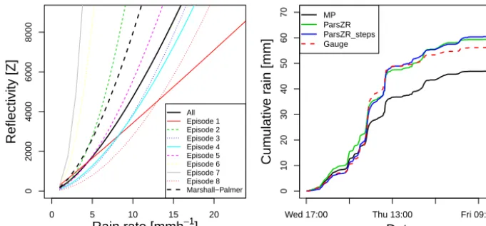
Figure 10.Left panel: all nonlinear fits together with the Marshall–PalmerZ–Rrelation. Right panel: accumulated rain for differentZ–R
relations applied to reflectivity data that are corrected for calibration, static clutter and wet-radome attenuation.
tation. By making use of the effectiveZ–Rrelations shown in Fig. 9, much larger precipitation values are obtained. Fur-thermore, since these two episodes contain the rain with the highest rainfall intensities observed for this event at the loca-tion of the radar, these larger estimates have a strong effect on the total accumulated rainfall. The Marshall–Palmer re-lationship overestimates the amount of rainfall only during three episodes. Episodes 6 and 7 produce much less rain than would be expected using the Marshall–Palmer relation (M– P), while episode 2 yields slightly less rain compared to M– P for higher reflectivities. These results clearly illustrate the impact of DSD variability on the effectiveZ–Rrelations and the limited effectiveness of a applying a single static relation.
4.4.2 Application ofZ–Rrelations
The effects of applying the derivedZ–Rrelations are shown in the right panel of Fig. 10. In this figure, three different approaches have been applied. First, the standard Marshall– Palmer relationship is used (similar to Fig. 7). As a second approach, the event-based Z–R relation, obtained from all
Z andR data collected by the Parsivel®during this event, is used (top-left panel of Fig. 9). Using a single representa-tiveZ–R relationship leads to considerably more precipita-tion (59.6 mm) than M–P (47.1 mm) and results in an over-estimation of about 6 % in total accumulation as compared to the nearby rain gauge. As a third procedure, the eight in-dividual, optimal intra-event power-law relationships were applied. This leads to a total precipitation accumulation of 61.0 mm, which is an overestimation by 8.3 %. The results clearly reveal the positive impact of applying an event-based
Z–Rrelationship, which for the current event could success-fully be derived from surface observations obtained by a sin-gle disdrometer. It should also be noted that even though con-siderable variations in the DSD are observed between the different episodes, leading to variations in the effectiveZ–
Rrelationship, this does not further improve the event-based precipitation estimates.
4.5 Verification of the correction methods
Several statistical parameters were selected to give a sum-mary of the overall quality of the radar improvements com-pared to the rain gauge. These are the sum, relative mean bias and the coefficient of variation.
The sum is defined as the accumulated rain sum found from the different radar corrections:
Sum= N X
i=1
R(i)1t, (5)
whereR(i)is the rain intensity of the radar for the current time step and1t is the time interval in hours (i.e., 0.1667 h for 10 min values).
The relative mean bias is defined as the mean difference between 10 min rainfall intensities from the radar and the rain gauge, normalized by the average gauge intensity:
Bias= N P
i=1
(R(i)−G(i))
N P
i=1
G(i)
×100 %, (6)
whereG(i)is defined as the rain intensity of the gauge for the current time step.
intensi-Table 3.Rainfall sum (mm) from the radar, together with relative mean bias (%) and coefficient of variation (CV) (%) of 10 min rain-fall intensities from the rain gauge and the radar for different correc-tion combinacorrec-tions. Here, operacorrec-tional means the operacorrec-tional Doppler clutter-corrected data, raw means the uncorrected data, static the static-clutter-corrected data and wet the wet-radome-corrected data. M–P is the rain rate derived using the Marshall–Palmer equation.
Pars means the rain rate derived using theZ–Rrelation found from
all data of the Parsivel®. Finally, Pars steps is the same, but for all
episodes of the event, the derivedZ–Rvalues are used.
Sum Relative mean CV
(mm) bias (%) (%)
M–P Operational 25.8 −54.1 224
M–P raw 39.0 −30.8 206
M–P static 34.5 −38.8 205
M–P wet+static 47.1 −16.3 157
ParsZRwet+static 59.6 5.9 139
ParsZRsteps wet+static 61.0 8.3 123
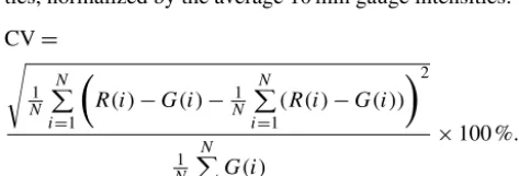
ties, normalized by the average 10 min gauge intensities:
CV= (7)
s
1 N
N P
i=1
R(i)−G(i)− 1
N N P
i=1
(R(i)−G(i))
2
1 N
N P
i=1
G(i)
×100 %.
Table 3 illustrates the above-mentioned statistics for sev-eral combinations of corrections. The operational product (applied M–P and Doppler clutter filter) gives rise to a large underestimation by the radar and the worst performance. Not performing any kind of clutter correction leads to better re-sults as compared to the operational product, both in total rainfall, standard deviation as well as bias. If a wet-radome correction is applied to the static-clutter-corrected images, all statistics improve and the difference between rain gauge and radar decreases from 38.8 to 16.3 %. By converting the cor-rected reflectivity data using the Parsivel®-inferredZ–R re-lation, further improvements in the quality of the radar prod-uct are obtained. Now the differences become very small, both in terms of bias and coefficient of variation. This is also apparent from the difference in rainfall accumulations. While the radar now slightly overestimates the gauge, this value is much closer to the rainfall accumulation than when using M– P. Finally, the use of a different Parsivel®-derivedZ–R rela-tion for each episode gives a larger overestimarela-tion compared to the rain gauge. The coefficient of variation also decreases with each improvement. The effect would have been even larger if time steps without precipitation were removed from the data. This reduces the CV for the full correction from 123 to 81 %.
The final results for both correction methods based on the Parsivel®-derived Z–R relations are comparable to the
ob-servations by the rain gauge. The comparison between both instruments is remarkably close, especially if one takes the differences between both instruments, their effective sam-pling volumes and the impact of elevation differences into account. It should be noted that rain gauges give point mea-surements over a period and radar data are instantaneous measurements of a volume in the air, so comparison is not straightforward (Kitchen and Blackall, 1992; Ciach and Kra-jewski, 1999; Bringi and Rico-Ramirez, 2011). While the sampling time interval can cause errors in radar rainfall esti-mation, especially during convective situations (Fabry et al., 1994), the space–time structure of the precipitation for this event was such that this had only a minor effect on the re-sults.
5 Summary and conclusions
In the current study, close-range quantitative precipitation es-timation (QPE) by radar was analyzed. By focussing specif-ically on regions close to the radar, the effects of rain-induced attenuation, VPR and non-uniform beam filling are expected to be small, allowing errors due to calibration, clutter, wet-radome attenuation and Z–R variability to be addressed. It was found that for this event the operational clutter-corrected radar product underestimated the rainfall accumulation by 54.1 % compared to the rain gauge using a standard Marshall–PalmerZ–R relation. The operational time-domain Doppler clutter filter used by KNMI is shown to erroneously filter some of the rain as well. By correcting radar volume data for clutter using a simple static clutter fil-ter, the underestimation reduces to 38.8 %. Further improve-ment is obtained when the data are corrected for wet-radome attenuation by using a stable clutter target close to the radar as reference. These two corrections, along with a correction for calibration error, jointly give an optimal estimated reflec-tivity from the radar. Applying M–P, this resulted in a 16.3 % underestimation with respect to the rain gauge.
Finally, theZ–Rrelation was analyzed in detail to investi-gate if this could improve results. This was done by fitting a power-law function usingZandRvalues obtained from the Parsivel®disdrometer and applying this to the fully corrected radar reflectivities. This resulted in a slight overestimation of 5.9 %. Additionally, the event was split up into eight different episodes based on DSD data and radar images. A dedicated
The results presented in this work clearly show that the rainfall estimation capabilities of the radar have tremendous potential, if errors can be properly corrected for. Even at close ranges from the radar, multiple sources of error are shown to significantly affect radar rainfall estimates. The multiplicative nature of most of these errors means that their effect on rainfall estimates is greatest at high rainfall intensi-ties. It is shown here that using a time-domain Doppler clutter filter on all radar pixels causes significant underestimation. Using an operational algorithm that is more selective in clut-ter filclut-tering (e.g., CMD; see Hubbert et al., 2009), or using a Doppler filter with spectral reconstruction (e.g., Nguyen and Chandrasekar, 2013) will likely reduce this problem. Appli-cation of the technique used to correct for the wet-radome attenuation to an entire radar image is not recommended be-cause wet-radome attenuation may be strongly dependent on azimuth, which probably depends on the wind speed and di-rection. It is relevant to study this in more detail because wet-radome attenuation can cause major (i.e., 3–4 dB; see Fig. 7) underestimation of precipitation. As both convective and stratiform precipitation were observed in this study, it is expected that the results also hold for more than just this event and can be considered to be quite general. This case did not contain solid precipitation, like hail or snow, at ground level. It would therefore be very interesting to also explore the effect of these precipitation types.
The availability of a disdrometer enabled the derivation of intra-event Z–R relations for selected periods. The cur-rent study showed that this led to improved rainfall esti-mates as obtained from the radar, instead of using the stan-dard Marshall–Palmer relationship. The current work only focussed on the impact of an event-basedZ–Rrelationship close to the radar. Recently, Hazenberg et al. (2014, 2016) ex-tended this approach to the whole radar domain for summer-time precipitation, identifying the benefits and limitations of using the disdrometer information. For convective precipi-tation, the potential benefit of these instruments was small. This is because the locations of these cells do not correspond to the location of the disdrometer. However, for widespread stratiform precipitation, by making use of observations ob-tained by a single disdrometer, a much better correspondence with the rain gauges was observed as compared to applying a single staticZ–Rrelationship. These results show both the possibilities and limitations of making use of disdrometer ob-servations to derive information on the event-basedZ–R re-lationship.
6 Data availability
Weather radar data are available from the KNMI Data Centre (http://data.knmi.nl). Rain gauge and disdrometer data are available upon request by sending an e-mail to [email protected].
Acknowledgements. Financial support for this work was provided by the Netherlands Space Office (NSO) and Netherlands Orga-nization for Scientific Research (NWO) through grant EO-058. The authors would also like to thank Marijn de Haij of KNMI for providing the disdrometer data used in this paper.
Edited by: G. Vulpiani
Reviewed by: M. Rico-Ramirez, N. I. Fox, M. Montopoli and one anonymous referee
References
Andrieu, H., Delrieu, G., and Creutin, J.-D.: Identification of verti-cal profiles of radar reflectivity for hydrologiverti-cal applications us-ing an inverse method, Part 2: Sensitivity analysis and case study, J. Appl. Meteorol., 34, 240–259, 1995.
Andrieu, H., Creutin, J.-D., and Faure, D.: Use of a weather radar for the hydrology of a mountainous area, Part I: Radar measure-ment interpretation, J. Hydrol., 193, 1–25, 1997.
Battan, L. J.: Radar Observation of the Atmosphere, University of Chicago Press, 324 pp., 1973.
Beekhuis, H. and Holleman, I.: From pulse to product, highlights of the digital-IF upgrade of the Dutch national radar network, Proceedings of the 5th European Conference on Radar in Meteo-rology and HydMeteo-rology, Helsinki, Finland, 30 June–4 July, 2008. Beekhuis, H. and Leijnse, H.: An operational radar monitoring tool,
proceedings of the 7th European Conference on Radar in Mete-orology and Hydrology, Toulouse, France, paper 47DQ, 25–29 June, 2012.
Berenguer, M., Sempere Torres, D., Corral, C., and Sánchez-Diezma, R.: A fuzzy logic technique for identifying non-precipitating echoes in radar scans, J. Atmos. Ocean. Tech., 23, 1157–1180, 2005.
Berne, A. and Uijlenhoet, R.: A stochastic model of range profiles of raindrop size distributions: application to radar attenuation correction, Geophys. Res. Lett., 32, L10803, doi:10.1029/2004GL021899, 2005.
Berne, A., Delrieu, G., Creutin, J.-D., and Obled, C.: Temporal and spatial resolution of rainfall measurements required for urban hy-drology, J. Hydrol., 299, 166–179, 2004.
Bouilloud, L., Delrieu, G., Boudevillain, B., Borga, M., and Zanon, F.: Radar rainfall estimation for the post-event analysis of a Slovenian flash-flood case: application of the Mountain Refer-ence Technique at C-band frequency, Hydrol. Earth Syst. Sci., 13, 1349–1360, doi:10.5194/hess-13-1349-2009, 2009. Brauer, C. C., Teuling, A. J., Overeem, A., van der Velde, Y.,
Hazen-berg, P., Warmerdam, P. M. M., and Uijlenhoet, R.: Anatomy of extraordinary rainfall and flash flood in a Dutch lowland catch-ment, Hydrol. Earth Syst. Sci., 15, 1991–2005, doi:10.5194/hess-15-1991-2011, 2011.
Bringi, V. N. and Chandrasekar, V.: Polarimetric Doppler Weather Radar: Principles and Applications, Cambridge University Press, 2001.
Bringi, V. N., Chandrasekar, V., Balakrishnan, N., and Zrnic, D. S.: An examination of propagation effects in rainfall on radar mea-surements at microwave frequencies, J. Atmos. Ocean. Tech., 7, 829–840, 1990.
Chapon, B., Delrieu, G., Gosset, M., and Boudevillain, B.: Variabil-ity of rain drop size distribution and its effect on the Z-R rela-tionship: A case study for intense Mediterranean rainfall, Atmos. Res., 87, 52–65, 2008.
Ciach, G. J.: Local random errors in tipping-bucket rain gauge mea-surements, J. Atmos. Ocean. Tech., 20, 752–759, 2003. Ciach, G. J. and Krajewski, W. F.: On the estimation of radar rainfall
error variance, Adv. Water Resour., 22, 585–595, 1999. de Haij, M. and Wauben, W. F.: Investigations into the
improve-ment of automated precipitation type observations at KNMI, Pro-ceedings of the WMO Technical Conference on Meteorologi-cal and Environmental Instruments and Methods of Observation, Helsinki, Finland, 2–8 September 2010, Paper 3(2), 2010.
Delrieu, G., Creutin, J.-D., and Saint-André, I.: MeanK–R
relation-ships: Practical results for typical weather radar wavelengths, J. Atmos. Ocean. Tech., 8, 467–476, 1991.
Delrieu, G., Caoudal, S., and Creutin, J.-D.: Feasibility of us-ing mountain return for the correction of ground-based X-band weather radar, J. Atmos. Ocean. Tech., 14, 368–385, 1997. Delrieu, G., Boudevillain, B., Nicol, J., Chapon, B., Kirstetter,
P. E., Andrieu, H., and Faure, D.: Bollène-2002 experiment: Radar quantitative precipitation estimation in the Cévennes-Vivarais region (France), J. Appl. Meteorol. Clim., 48, 1422– 1447, doi:10.1175/2008JAMC1987.1, 2009.
Fabry, F., Austin, G., and Tees, D.: The accuracy of rainfall esti-mates by radar as a function of range, Q. J. Roy. Meteor. Soc., 118, 435–453, 1992.
Fabry, F., Bellon, A., Duncan, M. R., and Austin, G. L.: High reso-lution rainfall measurements by radar for very small basins: the sampling problem reexamined, J. Hydrol., 162, 415–428, 1994. Fulton, R., Breidenbach, J., Seo, D.-J., Miller, D., and O’Bannon,
T.: The WSR-88D rainfall algorithm, Weather Forecast., 13, 377–395, 1998.
Germann, U.: Radome attenuation–a serious limiting factor for quantitative radar measurements?, Meteorol. Z., 8, 85–90, 1999. Gorgucci, E. and Chandrasekar, V.: Evaluation of Attenuation Cor-rection Methodology for Dual-Polarization Radars: Application to X-Band Systems, J. Atmos. Ocean. Tech., 22, 1195–1206, doi:10.1175/JTECH1763.1, 2005.
Gosset, M. and Zawadzki, I.: Effect of nonuniform beam filling on the propagation of the radar signal at X-band frequencies, Part
I: Changes in thek(Z)relationship, J. Atmos. Ocean. Tech., 18,
1113–1126, 2001.
Habib, E., Krajewski, W. F., and Kruger, A.: Sampling errors of tipping bucket rain gauge measurements, J. Hydrol. Eng., 6, 159– 166, doi:10.1061/(ASCE)1084-0699(2001)6:2(159), 2001. Hazenberg, P., Leijnse, H., and Uijlenhoet, R.: Radar rainfall
es-timation of stratiform winter precipitation in the Belgian Ar-dennes, Water Resour. Res., 47, 1–15, 2011a.
Hazenberg, P., Ya, N., Boudevillain, B., and Uijlenhoet, R.: Scal-ing of raindrop size distributions and classification of radar reflectivity-rain rate relations in intense Mediterranean precipi-tation, J. Hydrol., 402, 179–192, 2011b.
Hazenberg, P., Torfs, P. J. J. F., Leijnse, H., Delrieu, G., and Ui-jlenhoet, R.: Identification and uncertainty estimation of vertical
reflectivity profiles using a Lagrangian approach to support quan-titative precipitation measurements by weather radar, J. Geophys. Res., 118, 10243–10261, 2013.
Hazenberg, P., Leijnse, H., and Uijlenhoet, R.: The impact of re-flectivity correction and accounting for raindrop size distribution variability to improve precipitation estimation by weather radar for an extreme low-land mesoscale convective system, J. Hydrol., 519, 3410–3425, doi:10.1016/j.jhydrol.2014.09.057, 2014. Hazenberg, P., Leijnse, H., and Uijlenhoet, R.: Contribution of
long-term accounting for raindrop size distribution variations on quan-titative precipitation estimation by weather radar: Disdrometers vs parameter optimization, Adv. Water Resour., submitted, 2016. Hitschfeld, W. and Bordan, J.: Errors inherent in the radar mea-surement of rainfall at attenuating wavelengths, J. Meteorol., 11, 58–67, 1954.
Holleman, I. and Beekhuis, H.: Review of the KNMI clutter removal scheme, Tech. Rep. TR-284, Royal Netherlands Meteorological Institute, available at: http://www.knmi.nl/publications/fulltexts/ tr_clutter.pdf, 2005.
Holleman, I., Huuskonen, A., Kurri, M., and Beekhuis, H.: Opera-tional monitoring of weather radar receiving chain using the sun, J. Atmos. Ocean. Tech., 27, 159–166, 2010.
Hubbert, J. C., Dixon, M., and Ellis, S. M.: Weather radar ground clutter, Part II: Real-time identification and filtering, J. Atmos. Ocean. Tech., 26, 1182–1197, 2009.
Kitchen, M. and Blackall, M.: Representativeness errors in compar-isons between radar and gage measurements of rainfall, J. Hy-drol., 134, 13–33, 1992.
Kurri, M. and Huuskonen, A.: Measurements of the transmission loss of a radome at different rain intensities, J. Atmos. Ocean. Tech., 25, 1590–1599, 2008.
Leijnse, H., Uijlenhoet, R., van de Beek, C. Z., Overeem, A., Otto, T., Unal, C. M. H., Dufournet, Y., Russchenberg, H. W. J., Figueras i Ventura, J., Klein Baltink, H., and Holleman, I.: Pre-cipitation measurement at CESAR, The Netherlands, J. Hydrom-eteorol., 11, 1322–1329, doi:10.1175/2010JHM1245.1, 2010. Löffler-Mang, M. and Joss, J.: An optical disdrometer for measuring
size and velocity of hydrometeors, J. Atmos. Ocean. Tech., 17, 130–139, 2000.
Marsalek, J.: Calibration of the tipping-bucket raingage, J. Hydrol., 53, 343–354, 1981.
Marshall, J. S., Hitschfeld, W., and Gunn, K. L. S.: Advances in radar weather, Adv. Geophys., 2, 1–56, 1955.
Marzoug, M. and Amayenc, P.: A class of single- and dual-frequency algorithms for rain-rate profiling from a spaceborne radar, Part I: Principle and test from numerical simulations, J. Atmos. Ocean. Tech., 11, 1480–1506, 1994.
Morin, E., Krajewski, W. F., Goodrich, D. C., Gao, X., and Sorooshian, S.: Estimating rainfall intensities from weather radar data: The scale-dependency problem, J. Hydrometeorol., 4, 782– 796, 2003.
Nguyen, C. M. and Chandrasekar, V.: Gaussian model adaptive pro-cessing in time domain (GMAP-TD) for weather radars, J. At-mos. Ocean. Tech., 30, 2571–2584, 2013.
Overeem, A., Buishand, A., and Holleman, I.: Rainfall depth-duration-frequency curves and their uncertainties, J. Hydrol., 348, 124–134, doi:10.1016/j.hydrol.2007.09.044, 2008. Overeem, A., Buishand, A., and Holleman, I.: Extreme
using weather radar, Water Resour. Res., 45, W10424, doi:10.1029/2009WR007869, 2009.
Rhyzkov, A. V.: The impact of Bbeam broadening on the quality of radar polarimetric data, J. Atmos. Ocean. Tech., 24, 729–744, 2007.
Salles, C. and Creutin, J. D.: Instrumental uncertainties in Z-R re-lationships and raindrop fall velocities, J. Appl. Meteorol., 42, 279–290, 2003.
Saltikoff, E., Cho, J. Y. N., Tristant, P., Huuskonen, A., All-mon, L., Cook, R., Becker, E., and Joe, P.: The Threat to Weather Radars by Wireless Technology, B. Am. Meteorol. Soc., doi:10.1175/BAMS-D-15-00048.1, online first, 2015.
Sassi, M., Leijnse, H., and Uijlenhoet, R.: Sensitivity of power functions to aggregation: bias and uncertainty in radar rainfall retrieval, Water Resour. Res., 50, 8050–8065, doi:10.1002/2013WR015109, 2014.
Serrar, S., Delrieu, G., Creutin, J., and Uijlenhoet, R.: Mountain reference technique: Use of mountain returns to calibrate weather radars operating at attenuating wavelengths, J. Geophys. Res., 105, 2281–2290, doi:10.1029/1999JD901025, 2000.
Sevruk, B. and Nespor, V.: Empirical and theoretical assessment of the wind induced error of rain measurements, Water Sci. Tech., 37, 171–178, 1998.
Sevruk, B. and Zahlavova, L.: Classification system of precipitation gauge site Exposure: Evaluation and Application, Int. J. Clima-tol., 14, 681–689, 1994.
Steiner, M. and Smith, J. A.: Use of three-dimensional reflec-tivity structure for automated detection and removal of non-precipitating echoes in radar data, J. Atmos. Ocean. Tech., 19, 673–686, 2002.
Testud, J., Le Bouar, E., O. E., and Ali-Mehenni, M.: The rain pro-filing algorithm applied to polarimetric weather radar, J. Atmos. Ocean. Tech., 17, 332–356, 2000.
Thurai, M., Petersen, W. A., Tokay, A., Schultz, C., and Gatlin, P.: Drop size distribution comparisons between Parsivel and 2-D video disdrometers, Adv. Geosci., 30, 3–9, doi:10.5194/adgeo-30-3-2011, 2011.
Tokay, A., Bashor, P. G., and Wolff, K. R.: Error characteristics of rainfall measurements by collocated Joss-Waldvogel disdrome-ters, J. Atmos. Ocean. Tech., 22, 513–527, 2005.
Tokay, A., Petersen, W. A., Gatlin, P., and Wingo, M.: Compar-ison of Raindrop Size Distribution Measurements by Collo-cated Disdrometers, J. Atmos. Ocean. Tech., 30, 1672–1690, doi:10.1175/JTECH-D-12-00163.1, 2013.
Uijlenhoet, R.: Raindrop size distributions and radar reflectivity-rain rate relationships for radar hydrology, Hydrol. Earth Syst. Sci., 5, 615–628, doi:10.5194/hess-5-615-2001, 2001.
Uijlenhoet, R. and Berne, A.: Stochastic simulation experiment to assess radar rainfall retrieval uncertainties associated with atten-uation and its correction, Hydrol. Earth Syst. Sci., 12, 587–601, doi:10.5194/hess-12-587-2008, 2008.
Uijlenhoet, R., Steiner, M., and Smith, J. A.: Variability of raindrop size distributions in a squall line and implications for radar rain-fall estimation, J. Hydrometeorol., 4, 43–61, 2003.
Uijlenhoet, R., Porrà, J. M., Sempere Torres, D., and Creutin, J.-D.: Analytical solutions to sampling effects in drop size distribution measurements during stationary rainfall: Estimation of bulk rain-fall variables, J. Hydrol., 328, 65–82, 2006.
Ulbrich, C. W. and Lee, L. G.: Rainfall measurement error by
WSR-88D radars due to variations inZ–Rlaw parameters and the radar
constant, J. Atmos. Ocean. Tech., 16, 1017–1024, 1999. van de Beek, C. Z., Leijnse, H., Stricker, J. N. M., Uijlenhoet, R.,
and Russchenberg, H. W. J.: Performance of high-resolution X-band radar for rainfall measurement in The Netherlands, Hydrol. Earth Syst. Sci., 14, 205–221, doi:10.5194/hess-14-205-2010, 2010.
van de Beek, C. Z., Leijnse, H., Torfs, P. J. J. F., and Uijlenhoet, R.: Climatology of daily rainfall semi-variance in The Netherlands, Hydrol. Earth Syst. Sci., 15, 171–183, doi:10.5194/hess-15-171-2011, 2011a.
van de Beek, C. Z., Leijnse, H., Torfs, P. J. J. F., and Uijlenhoet, R.: Seasonal semi-variance of Dutch rainfall at hourly to daily scales, Adv. Water Resour., 15, 171–183, 2011b.
Vignal, B., Galli, G., Joss, J., and Germann, U.: Three methods to determine profiles of reflectivity from volumetric radar data to correct precipitation estimates, J. Appl. Meteorol., 39, 1715– 1726, 2000.
Wauben, W.: Precipitation amount and intensity measurements us-ing a windscreen, Tech. Rep. TR-262, R. Neth. Meteorol. Inst., De Bilt, the Netherlands, 2004.
Wauben, W.: KNMI contribution to the WMO laboratory inter-comparison of rainfall intensity gauges, Tech. Rep. TR-287, Royal Netherlands Meteorological Institute, De Bilt, the Nether-lands, available at: http://www.knmi.nl/bibliotheek/knmipubTR/ TR287.pdf, 2006.
WMO: Guide to meteorological instruments and methods of obser-vation, Tech. Rep. WMO-N0. 8, 6th Edn., World Meteorological Organization, Geneva, Switzerland, 1996.
Yuter, S. E., Kingsmill, D., Nance, L. B., and Löffler-Mang, M.: Observations of precipitation size and fall speed characteristics within coexisting rain and wet snow, J. Appl. Meteorol., 45, 1450–1464, doi:10.1175/JAM2406.1, 2006.