www.nonlin-processes-geophys.net/14/763/2007/ © Author(s) 2007. This work is licensed
under a Creative Commons License.
Nonlinear Processes
in Geophysics
A comparison of the performance of 4D-Var in an explicit and
implicit version of a nonlinear barotropic ocean model
A. D. Terwisscha van Scheltinga and H. A. Dijkstra
Institute for Marine and Atmospheric research Utrecht, Department of Physics and Astronomy, Utrecht University, Princetonplein 5, 3584 CC, Utrecht, The Netherlands
Received: 4 July 2007 – Revised: 1 November 2007 – Accepted: 3 November 2007 – Published: 30 November 2007
Abstract. A comparison is made of the performance of the four-dimensional variational data assimilation (4D-Var) method in an explicit and implicit version of a barotropic quasi-geostrophic model of the wind-driven double-gyre ocean circulation. As is well known, implicit methods have the advantage that relatively large time steps can be taken with respect to explicit methods, but the computational costs of each time step is larger. We focus here on two issues: (i) the computational efficiency in the range of time steps where the chosen explicit method is still numerically stable and (ii) the performance of 4D-Var in the implicit model for time steps out of reach for the explicit model. For the same time step1t and the same number of points nper assimilation interval, the analyses in the implicit model is always more accurate than that in the explicit model. Due to this prop-erty the use of 4D-Var combined with the implicit model can be computationally more efficient than its use in the explicit model.
1 Introduction
The four-dimensional variational data assimilation method, 4D-Var, is now widely applied in meteorology and phys-ical oceanography. It is a method in which information that is present in observations is combined with the evolu-tion determined by a particular ocean, atmosphere or climate model. The 4D-Var method is routinely applied at ECMWF in weather forecasting (Rabier et al., 2000; Mahfouf and Ra-bier, 2000; Klinker et al., 2000). In operational oceanogra-phy, for example within the French Mercator project (Weaver et al., 2003; Vialard et al., 2003), the use of observations to initialize ocean circulation models results in better fore-casts. The Estimating the Circulation and Climate of the Correspondence to: A. D. Terwisscha van Scheltinga ([email protected])
the last decade. For example, implicit quasi-geostrophic and shallow-water models of the wind-driven ocean circu-lation have been used to investigate the bifurcation behavior of the double-gyre circulation (Dijkstra and Katsman, 1997; Schmeits and Dijkstra, 2000). A hierarchy of fully-implicit models of the thermohaline ocean circulation has helped clar-ify the role of different equilibria in the hysteresis behavior of the global ocean circulation (Dijkstra et al., 2004). The immediate advantage of these methods is that much larger time steps can be taken than with explicit methods. A few years ago 4D-Var was implemented in fully implicit mod-els (Terwisscha van Scheltinga and Dijkstra, 2005). In this implementation, the adjoint model is easily derived from the implicit time-stepping scheme, and the choice of the time step is not limited by numerical stability but by accuracy. In this paper, we compare the performance of the implemen-tation of 4D-Var in an implicit version (abbreviated below with i4D-Var) of a barotropic quasi-geostrophic model of the double-gyre wind-driven circulation with 4D-Var applied to an explicit version (abbreviated below with e4D-Var) of the same model. The aim of the comparison is to investigate whether implicit methods provide useful alternatives in prob-lems where variational data-assimilation techniques are used.
2 Model and methods
In the first subsection below (Sect. 2.1), we provide the model of the wind-driven ocean circulation which is used in this study. Next, we provide a basic overview of the 4D-Var method (Sect. 2.2) such that the differences between the im-plementation of 4D-Var in the implicit and explicit versions of the ocean model in Sect. 2.3 can be explained more easily. 2.1 Barotropic wind-driven ocean flows
Consider a rectangular ocean basin of sizeL×L having a constant depthD. The basin is situated on a midlatitudeβ -plane with a central latitudeθ0=45◦N and Coriolis param-eterf0=2sinθ0, whereis the rotation rate of the Earth. The meridional variation of the Coriolis parameter at the lat-itudeθ0 is indicated byβ0. The densityρ of the water is constant and the flow is forced at the surface through a wind-stress vectorT=τ0[τx(x, y), τy(x, y)]. The governing equa-tions are non-dimensionalized using a horizontal length scale L, a vertical length scaleD, a horizontal velocity scaleU, the advective time scaleL/U and a characteristic amplitude of the wind-stress vector,τ0. The effect of deformations of theocean-atmosphere interface on the flow is neglected.
The dimensionless barotropic quasi-geostrophic model of the flow for the vorticityζ and the geostrophic streamfunc-tionψis (Pedlosky, 1987)
h∂
∂t +u ∂ ∂x+v
∂ ∂y
i
[ζ+βy] =Re−1∇2ζ+ατ
∂τy ∂x − ∂τx ∂y , (1a)
ζ = ∇2ψ, (1b)
where the dimensionless horizontal velocities are given by u=−∂ψ/∂y andv=∂ψ/∂x. The parameters in Eq. (1a) are the Reynolds numberRe, the planetary vorticity gradient pa-rameterβ and the wind-stress forcing strengthατ. These parameters are defined as:
Re= U L AH
; β= β0L 2
U ; ατ = τ0L
ρDU2 (2)
whereg is the gravitational acceleration andAH is the lat-eral friction coefficient. We assume no-slip conditions on the east-west boundaries and slip on the north-south boundaries. The boundary conditions are therefore given by
x=0, x=1:ψ= ∂ψ
∂x =0, (3a)
y=0, y=1:ψ=ζ =0. (3b)
The wind-stress forcing is prescribed as renewcommand3b3a τx(x, y)=−1
2π cos 2πy, (4b)
τy(x, y)=0
, (4b)
and the zonal wind stress is symmetric with respect to the mid-axis of the basin (the standard double-gyre case). When the horizontal velocity scale is based on a Sverdrup balance of the flow, i.e.,
U= τ0 ρDβ0L
, (5)
it follows thatατ=β and two free parameters result (Ped-losky, 1987), for example the dimensionless boundary layer thicknessesδ2I=1/βandδM3=1/(βRe). A standard set of pa-rameter values has been chosen (Table 1) that are similar to those in Dijkstra and Katsman (1997) and for these parame-ters,ατ=β=2.8×10³.
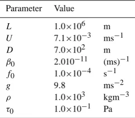
Table 1. Standard values of the parameters for the barotropic quasi-geostrophic ocean model.
Parameter Value
L 1.0×10⁶ m
U 7.1×10⁻³ ms−1
D 7.0×10² m
β0 2.010−11 (ms)−1
f0 1.0×10⁻⁴ s−1
g 9.8 ms−2
ρ 1.0×10³ kgm−3
τ0 1.0×10⁻¹ Pa
for 30<Re<52. Near Re=52 both asymmetric states be-come unstable due to the occurrence of Hopf bifurcations; for 52<Re<74 stable periodic orbits exist. The solutions become quasi-periodic forRe>74 and irregular for higher values ofRe; the route to chaos is through a homoclinic or-bit (Simonnet et al., 2005).
2.2 The 4D-Var method
The incremental formulation of the 4D-Var method as de-scribed in Courtier et al. (1994) is used and the notation is adapted from Ide et al. (1997). Letwbe the state vector con-sisting of model variables that are to be estimated by com-bining model dynamics and observations. Ifwbis the back-ground state andδwis the increment on the background state, then we want to determineδwsuch that the resulting statew defined by
w=wb+δw (6)
is “close” to observations. In the 4D-Var approach, the analysiswa is defined as the state vector which minimizes both the distance to the background wb(t0) and to the time-sequence of observationsyi, i=1,· · ·, nin the interval t0≤ti≤tn. Hence, this defines a cost functionJ as (Courtier et al., 1994):
J (δw)=δwTB−1δw+ n X
i=0
dTi R−i 1di, (7)
where the departuresdi are defined as:
di =yi−HiM(ti, t0)(wb(t0))−HiM(ti, t0)δw(t0). (8) The matrices B and Ri in Eq. (7) are the covariances of the background and the observation errors. The operator M(ti, t0)in Eq. (8) represents the evolution operator, such that
w(ti)=M(ti, t0)(w(t0)), (9) andHi in Eq. (8) is the observation operator. The lineariza-tion of the operatorsM(ti, t0)andHiaround the background
(a)
(b)
(c)
(a)
(b)
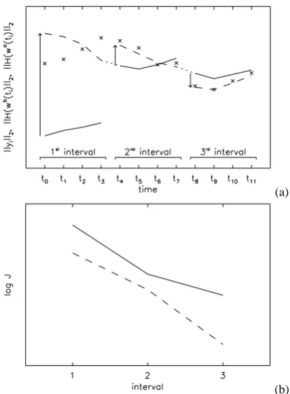
Fig. 2. Sketch of the 4D-Var method, where an assimilation in-terval has been divided into three subinin-tervals. (a)kH (wb(ti)k2 andkH (wa(ti)k2, theL2-norm of the projection of the background wb(ti) (solid) and analysis wa(ti) (dashes) on the observations space; theL2-norm of the observationsmat hbf yi(crosses) and the optimal incrementsδwa(arrows). (b) the initial (solid) and final (dashed) value of the cost function.
state are denoted by M(ti, t0)and Hi, respectively. Ifδwais defined as the solution of the optimization problem
δwa=min
δw J (δw), (10)
then the analysis is given by
wa(t0)=wb(t0)+δwa. (11) To solve the optimization problem Eq. (10) on each subinter-val, the gradient of the cost functionJ in Eq. (7), i.e.,
∇J (δw)=2w−1δw− n X
i=0
MT(ti,t0)HTiR −1
i di, (12)
has to be calculated.
To clarify the terminology used below, an illustration of the 4D-Var method has been provided in Fig. 2a. In this figure, the observations (crosses) are shown on an ex-ample assimilation interval t1≤ti≤t12. This interval has been divided into three subintervals, each with four points (n=4). For every interval the background trajectorywb(ti)
(solid), the optimal increment δwa (arrows) and the anal-ysis wa(t
i) (dashed) are shown. The background on the first interval is given. For the other intervals, the back-ground is calculated from the analysis on the previous in-terval:wb(tn+1)=M(tn+1, tn)(wa(tn)). On each interval the minimization problem Eq. (10) is solved. Due to the depen-dence of the cost function on the background, the increment and the observations, the initial and the final value of the cost function will vary over the subintervals (Fig. 2b).
2.3 Explicit and implicit implementations
The equations Eq. (1a) and boundary conditions Eq. (3a) are spatially discretized using a control-volume method on an equidistant N×M grid. For the explicit integration the second-order Adams-Bashforth time discretization is used in which the first step, for each assimilation interval, is an Euler step. In this explicit implementation (e4D-Var) the cost function is first computed by forward evolution over the time interval. The gradient is then evaluated by integrating the adjoint model, with evolution MT(ti, ti−1)and forcing HTi R−i 1di, backwards in time. For the implicit integration
tolerancem:
Jk−1−Jk < m(1+ |Jk|), (13a) kδwk−1−δwkk< m1/2(1+ kδwkk), (13b) k∇Jkk ≤m1/3(1+ |Jk|), (13c) wherekis the iteration index. For the optimality tolerance in E04DGF, a value ofm=10−5was chosen.
3 Comparison between i4D-Var and e4D-Var
In this section, we will compare the performance of i4D-Var and e4D-Var using the barotropic quasi-geostrophic ocean model. The specific set-up is described in Sect. 3.1 and re-sults for a standard case, with a fixed time step1tand a fixed number of points per assimilation interval n, in Sect. 3.2. The changes in performance when1t andnare varied are presented in Sects. 3.3 and 3.4, respectively and in Sect. 3.5 the overall computational efficiency of 4D-Var in the implicit and explicit model is compared.
3.1 Specific case
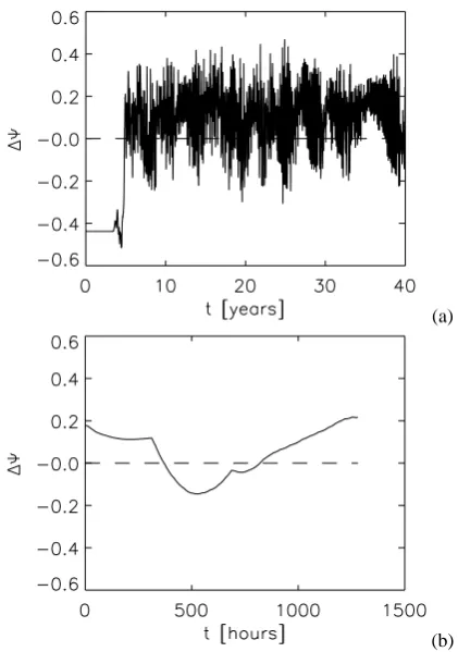
For a value of Refar into the irregular regime (Re=120), results of a 40 year time integration are shown in Fig. 3a. The quantity19on the vertical axis in Fig. 3a is a measure of the asymmetry of the streamfunctionψwith respect to the mid axis of the basin and it is defined as:
19= max(ψ )+min(ψ )
max(ψ,−ψ ) . (14)
A positive value of 19 indicates a downward jet-displacement, while a negative value of19 indicates an up-ward jet-displacement. In these computations, a time step of 1t=15 min was used for both the implicit and the explicit integration of the model. Both methods give near identical results such that the curves in Fig. 3a are indistinguishable.
The unstable jet-up steady state forRe=120 was chosen as the initial state att=0. Although the flow stays close to the initial state for the first few years, the behavior becomes ir-regular in time with frequent changes between upward and downward jet-displacement. For the comparison between the two 4D-Var implementations, we have derived the “ob-servations” from the 1200 h window after 10 years of inte-gration; the value of19 of these “observations” is plotted in Fig. 3b. Although the computed trajectories were nearly indistinguishable, for consistency the i4D-Var observations were taken from the implicit time-integration, while for e4D-Var they were taken from the explicit time-integration. The 1200 hour interval of observations is broken into subinter-vals, each withn points. On each of the subintervals, the minimization problem Eq. (10) is solved with the initial con-dition as control variables (cf. Fig. 2). For the covariances matrices, we have chosen (for simplicity) that B=Ri=I for
(a)
(b)
Fig. 3. The asymmetry19of the streamfunction for: (a) a time-integration of 40 years, starting from a unstable jet-up steady state; and (b) a 1200 h window after year 10 in (a); the latter values serve as the observations.
i=1,· · ·, n. The identity operator was chosen for the obser-vation operator (H=I), which means that we use all the ob-servations of the streamfunction. As initial background state we have chosen the unstable jet-up steady state atRe=120; this is the starting point of the time-series shown in Fig. 3a. For each interval the first guess of the minimization was taken asδw=0.
3.2 Accuracy
observa-(a)
(b)
(c)
(d)
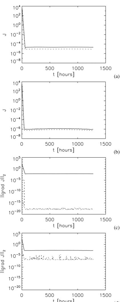
Fig. 4. Results for1t=2 h and 2 points per interval. (a) Initial value (solid) and final value (dashed) of the cost function for each mini-mization as evaluated by e4D-Var. (b) Initial value (solid) and final value (dashed) of the cost function for each minimization as eval-uated by i4D-Var. (c) Initial value (solid) and final value (dashed) of theL2norm of the gradient of the cost function for each mini-mization as evaluated by e4D-Var. (d) Initial value (solid) and final value (dashed) of theL2norm of the gradient of the cost function for each minimization as evaluated by i4D-Var.
tions and only a small correction on the background is nec-essary. The difference in the value of the cost function (both initial and final) between both methods is about one order of magnitude, with the implicit method having the smallest value of the cost function. This is due to the different eval-uation of the cost function: for e4D-Var, the term involving the tangent linear model in (8) is evaluated at the beginning of each time interval, while in i4D-Var, both begin and end points of the interval are used. The initial and final value of theL2norm of the gradient∇J are shown for e4D-Var and i4D-Var in Fig. 4c and d, respectively. Again there is a sharp decrease initially followed by stabilization afterwards. The initial value of the norm of∇J is of the same order for both methods but there is a large difference in the magnitude of the final values. This is due to a difference in the evaluation of the gradient: for i4D-Var, the evaluation of the gradient requires 2nlinear systems to be solved which is done using an iterative scheme with an accuracyi=10−6. As a result, theL2norm of the gradient cannot become smaller thani for i4D-Var. Since for e4D-Var no systems have to be solved, the norm of the gradient can be several orders of magnitude smaller.
An indication of the computational cost for both 4D-Var implementations is provided in Fig. 5a. Here the CPU time (tcomp) needed for a minimization over one assimilation in-terval is plotted for1t=2 h andn=2 for both i4D-Var (solid) and e4D-Var (dashed). The i4D-Var method is on average a factor 1.5 more expensive in computational time than e4D-Var. There are, however, several peaks where the difference is more than a factor 2.5 or higher. For both implementa-tions, the cost function Eq. (7) is minimized using an iter-ative scheme, with the optimality tolerancem=10−5. The conditions on the convergence of the iterate, cost function and gradient are more difficult to satisfy for i4D-Var, since the accuracy of the gradient is limited by the tolerance of the iterative linear solver (i=10−6). Hence, more iterations are needed for i4D-Var than for e4D-Var in the optimization procedure. Time integration is also more expensive for i4D-Var, since two linear systems have to be solved for each time step: one during evaluation of the cost function and one dur-ing evaluation of the gradient. Both factors make i4D-Var more expensive than e4D-Var.
To summarize the results for the chosen time-step and the number of points per interval: both implementations are ca-pable of finding an accurate analysis. i4D-Var appears more accurate than e4D-Var for this value ofn and1t, but it is also more expensive.
3.3 Effect of1t
(a)
(b)
(c)
Fig. 5. The processor timetcomp needed for the minimization of cost functionJfor each assimilation interval (see Fig. 2). The value oftcompis plotted at the beginning of the intervals. (a) for1t=2 h andn=2. (b) for1t=16 h andn=2. (c) for1t=2 h andn=16. The solid curves represent the results from i4D-Var. The dashed curves represent the results from e4D-Var.
The latter value of1tis close to the limiting time step (based on the CFL criterion) of the explicit scheme of1t≈17 h. In each figure panel, the top two curves are calculated by e4D-Var, while the bottom two are calculated by i4D-Var. For all intervals, the values of the cost function (both initial and final) as calculated by e4D-Var are larger than those calcu-lated by i4D-Var. For the first intervals, the same behavior is observed for both implementations: a rapid decrease of the cost function (both initial and final) and a decrease of the cost function during minimization. After the rapid decrease, the value of the cost function stabilizes.
For i4D-Var, the curves are comparable for each time step, although there is a small increase in the value of both the
(a)
(b)
(c)
(d)
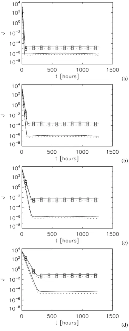
Fig. 6. Value of the initial (solid) and final (dashed) value of the cost function for several values of the time step andn=2. (a)1t=2 h. (b)1t=4 h. (c)1t=8 h. (d)1t=16 h. Curves marked with rect-angles denote results of e4D-Var. Curves without rectrect-angles denote results of i4D-Var.
(a)
(b)
(c)
(d)
Fig. 7. The difference between the observation and the analysis after minimization of the cost function for several values of the time step. (a)1t=2 h. (b) 1t=4 h. (c)1t=8 h. (d)1t=16 h. The solid curves represent the results from i4D-Var. The dotted curves represent the results from e4D-Var.
function stabilizes increases with increasing1t, for example by 4 orders of magnitude from1t=2 h to1t=16 h. This is
due to larger error propagation in the explicit scheme used in e4D-var for large1t. As a result, the evaluation of both the cost function and the gradient becomes less accurate. The same behavior can therefore be seen in theL2norm of the difference between analysis and observations, shown in Fig. 7 for different1t. For both implementations, there is again an increase in the equilibrium value of this norm with 1tbut the rate of increase is not as large as for the cost func-tion (Fig. 6). Hence, for increasing 1t the quality of the analysis decreases.
For1t=16 h and n=2, the CPU time per minimization is shown in Fig. 5b; again i4D-Var is more expensive than e4D-Var. The difference is on average a factor 2. This is a small increase compared to that found for1t=2 h andn=2 (Fig. 5a).
3.4 Effect ofn
Again using the same set-up as above, we now fix1t=2 h and vary the number of points per interval n=2,4,8 and n=16, i.e. the number of observations per subinterval within the 1200 h assimilation interval (cf. Fig. 2). In Fig. 8, the initial and final value of the cost function are plotted for both implementations. Again the two top curves are the results for e4D-Var, while the bottom two curves are for i4D-Var. In each panel we see a decrease of the cost function in the first few intervals followed by a stabilization. After this decrease there is a difference in behavior: i4D-Var is still able to im-prove the cost function, while e4D-Var fails to provide any improvement. The values of the cost function for e4D-Var are one order of magnitude larger than those for i4D-Var for n=2 and this difference increases to six orders of magnitude forn=16. For both implementations, the equilibrium values of the cost function increase withn. The rate of increase is one order of magnitude fromn=8 ton=16 for i4D-Var, but this is relatively small compared to that of e4D-Var.
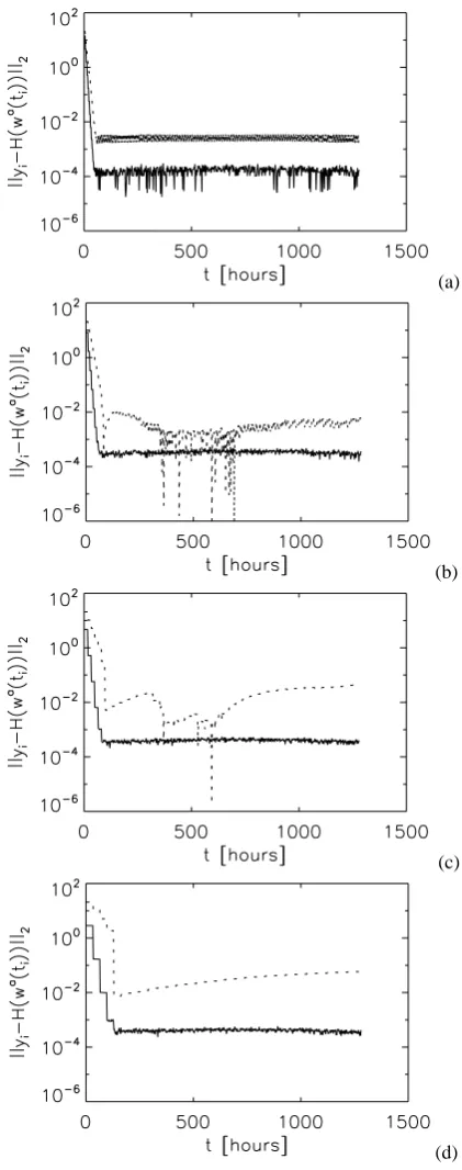
In Fig. 9, theL2norm of the difference between the anal-ysis and the observations is shown for each of value of n (as used in Fig. 8). For i4D-Var, this difference decreases in the first interval and then fluctuates around a constant value. With increasingnthe results of i4D-Var do not change much, apart from a small decrease of the size of the fluctuation and a small increase of the equilibrium value. For e4D-Var, how-ever, the equilibrium value does not remain constant with in-creasingnbut it slowly increases with time. In Fig 9b, there is a window in which theL2norm strongly fluctuates. To a lesser extent, this is also seen in Fig. 9c but it is absent in Fig. 9d. This window of fluctuations corresponds to a series of observations where the solution changes from jet-down to jet-up and back (Fig. 3b).
eval-(a)
(b)
(c)
(d)
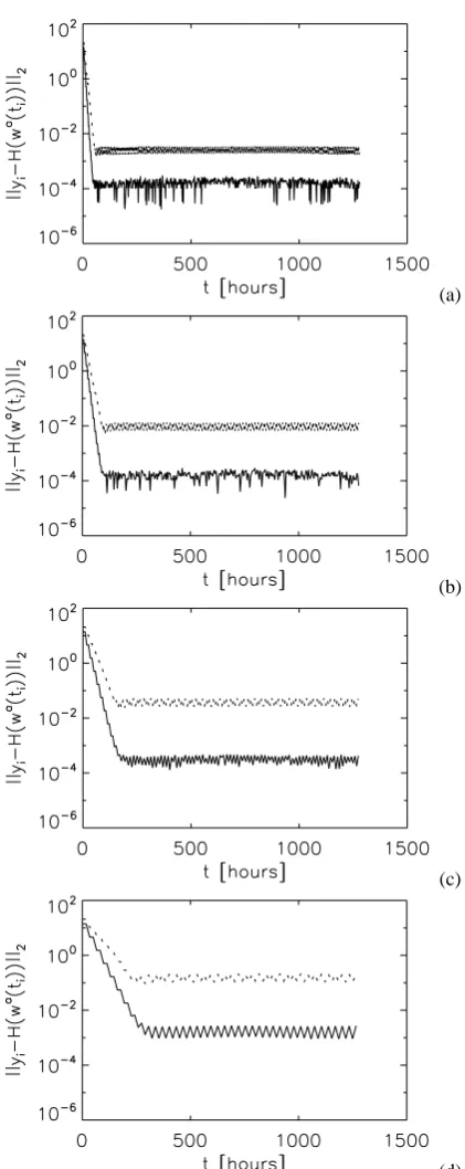
Fig. 8. Value of the initial (solid) and final (dashes) value of the cost function for differentn. (a)n=2. (b)n=4. (c)n=8. (d)n=16. Curves with rectangles denote results of e4D-Var. Curves without rectangles denote results of i4D-Var.
uation of cost function isn. In e4D-Var, the evaluation of the gradient requires 2nsteps;nfor the forward integration and nfor the backward integration with the adjoint model. As
(a)
(b)
(c)
(d)
Fig. 9. The difference between the observation and the analysis after minimization of the cost function for differentn. (a)n=2. (b)n=4. (c)n=8. (d)n=16. The solid curves represent the results from
i4D-Var. The dotted curves represent the results from e4D-Var.
qual-Table 2. The average accuracy of the analysis E=kyi−H (wa(ti))k2 and total processor time 6tcomp used for several combinations of the interval lengthnand time-step1t and for both explicit and implicit models. For three casestcomp is compared for the implicit and explicit method over the whole interval in Fig. 5; the superscripts a, b and c refer to the subpanels in Fig. 5.
n 1t[h] E 6tcomp[s] E 6tcomp[s] (implicit) (implicit) (explicit) (explicit)
2 2 0.0650 4925a 0.1323 2638a 4 2 0.0653 7819 0.2622 7970 8 2 0.0663 10976 0.5190 7299 16 2 0.0782 14570c 0.9819 4868c 2 4 0.1299 3440 0.2684 1347 4 4 0.1306 4553 0.5265 3046 8 4 0.1362 7088 1.0679 4241 16 4 0.1957 9019 2.0794 2918 2 8 0.2598 1678 0.5515 703 4 8 0.2626 2858 1.0695 1045 8 8 0.2989 4909 2.1996 1232 16 8 0.6143 8875 4.0994 1974 2 16 0.5200 1029b 1.1537 349b 4 16 0.5381 1942 2.1787 377 8 16 0.7654 4884 7.3980 548 16 16 2.2575 9237 8.8472 439
ity of the analysis of e4D-Var decreases faster (Fig. 9) with increasingncompared to i4D-Var. For 1t=2 h andn=16, the CPU time per minimization is plotted in Fig. 5c showing that i4D-Var is again more expensive than e4D-Var. After the first few intervals, the minimization scheme terminates after one iteration for e4D-Var since the NAG routine cannot find a direction where the residue is decreased, while condi-tions on the convergence are not satisfied. The minimization method is unable to find a converged minimum from the ini-tial guess (the iniini-tial increment) and the last value provided by the NAG routine is taken as the minimum. This leads to the lack of improvement in the cost function as seen in Figs. 8b–d.
3.5 Overall computational efficiency
In the previous results we saw that i4D-Var was more accu-rate than e4D-Var but also more expensive. For evaluating whether implicit methods provide a useful alternative for the range of1t smaller than the maximum value possible with the explicit method, one is interested in a comparison of the total processor time6tcompneeded to obtain a certain aver-age accuracy in the analysis over the whole time interval. As a measure of this average accuracy, we take the quantityE
defined as
E=kyi−H (wa(ti))k2 (15) Here the overbar indicates average of kyi−H (wa(ti))k2 taken over all the analyseswa(ti)found while assimilating
the observations in the 1200 hour window, using an interval length n and a time-step 1t. The total CPU time 6tcomp is the sum of the CPU times needed for each minimization along this interval. In Table 2, values of6tcomp andE are shown for several combinations of n and1t and for both explicit and implicit models. The values in Table 2 provide an indication of the computational costs for both methods to produce an analysis with a certain average accuracy. For example with e4D-Var, a value of E=0.13 is achieved for a value ofn=2 and1t=2 h at a computational cost of 2623 seconds. We also see that i4D-Var is more accurate than e4D-Var for the same value ofnand1tbut that it is about twice as expensive. To obtain about the same accuracy (E=0.13) with i4D-Var, we can use a larger time step and more points per interval (1t=2 andn=4) and for this case i4D-Var is only a factor 1.3 (3440/2638) more expensive than e4D-Var.
The values in Table 2 indicate that for i4D-Var,Edoes not increase much withnfor constant1t. Only for1t=16 there is a large increase forn=16, which is due to the relatively large weight of the initial adjustment. For i4D-Var, the total computational time increases approximately linearly withn. For e4D-VarEalways increases withndue to cumulative er-rors in the time-stepping. For the same1t,E for e4D-Var is always larger than that for i4D-Var. The total processor time for e4D-Var varies non-monotonically with increasing n. This is because for largenand1t the minimization ter-minates unsuccessfully due to inaccuracies in the integration method. From Table 2, we also see that for the particular model used here, i4D-Var can be more efficient than e4D-Var even in the range of values of1t below the CFL limit. For example, if a value ofE=0.52 is desired, we could use n=2 and1t=16 h for i4D-Var which would cost 1029 s. For the samen, we would have to use a1t=4 h with e4D-Var to obtain approximately the same value ofE, which would cost 1347 s.
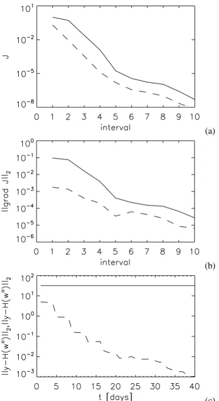
4 Performance of i4D-Var
of the model forRe=25. The background model is initial-ized with the steady-state solution atRe=20 and also run for Re=20. With i4D-Var approach, we assimilate observations obtained at one value ofRewithin the model which is run with a “wrong” value forRe. The initial increments for each assimilation interval are taken equal to zero and the observa-tion error covariance matrices Ri,i=1,· · ·,n are taken equal
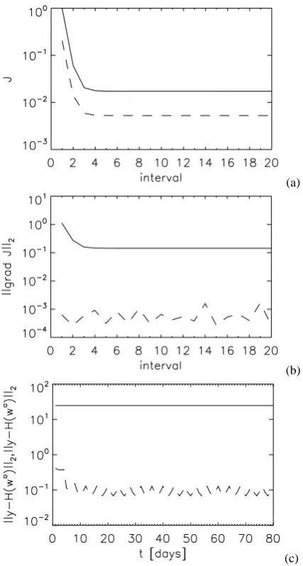
to the identity matrix I. A large decrease between the initial and final values of the cost function (Fig. 10a) and theL2 norm of the gradient (Fig. 10b) occurs. After the first four intervals, the value of the cost function stabilizes and the as-similation method cannot improve the analysis anymore. The difference between the observations and the analysis also sta-bilizes after a few intervals (Fig. 10c). This stabilization at a relatively large error is due to the fact that the background model has an unique steady solution atRe=20. Therefore, it is not possible to find an analysis that perfectly fits the ob-servations (forRe=25), since the observations are derived from a different steady solution. Although the ‘wrong’ back-ground model will not allow a perfect fit, i4D-Var finds an analysis which improves the solution of the “badly tuned” model to be closer to the observations.
Next, we consider how 4D-Var performs under case (ii) of a solution mismatch. As discussed earlier, for 30<Re<52, the barotropic ocean model has two stable steady solutions (cf. Fig. 1b, c). ForRe=50, which is in this multiple equi-libria regime, we synthesize “observations” from the jet-up solution in Fig. 1b, while we initialize the background model with the jet-down solution in Fig. 1c. The aim is to test whether the assimilation method is able to find the correct stable equilibrium, while being initialized with the “wrong one”. The initial increment for each interval is again taken equal to be zero and again the covariance matrices Ri,i=1,· · ·,n are taken to be the identity matrix I. For each
interval, there is a large difference between the initial and final value of the cost function (Fig. 11a) and theL2 norm of its gradient (Fig. 11b). A decrease of the initial and fi-nal values for each successive interval occurs, indicating that the analysis converges towards the observations. In Fig. 11c, the norm of the difference between the observations and the analysis converges towards zero. This indicates that i4D-Var is able to find an analysis which is a perfect fit to the obser-vations in this case.
Finally, we consider case (iii) for which noise is added to the observations. The steady stateψ forRe=25 is perturbed by adding noise to obtain the “observations”
yi =ψ+Ni(0,max|ψ|I), (16) where the maximum is taken over all the gridpoints and each Ni(µ,C) is a Gaussian distribution, whereµ is the mean and C the covariance matrix. The model is run (with a time-step of 24 h) atRe=25 and initialized with the steady-state solutionψ. For every assimilation interval, the initial incre-ment is taken equal to zero and the observation error
covari-(a)
(b)
(c)
Fig. 10. The solution mismatch case for Re=50. In this case, the “observations” are from Fig. 1c while the model is initialized with the solution in Fig. 1b. (a) Initial value (solid) and final value (dashed) of the cost function. (b) Initial value (solid) and final value (dashed) of the norm of the gradient. (c) Norms of the difference between the data and the model (solid) without assimilation and the data and the analysis (dashed) after assimilation.
ance matrix is taken as the covariance of the noise, i.e. for i=1, ..., n,
Ri =max|ψ| I. (17)
(a)
(b)
(c)
Fig. 11. The solution mismatch case forRe=50. In this case, the ‘observations’ are from Fig. 1c while the model is initialized with the solution in Fig. 1b. (a) Initial value (solid) and final value (dashed) of the cost function. (b) Initial value (solid) and final value (dashed) of the norm of the gradient. (c) Norms of the difference between the data and the model (solid) without assimilation and the data and the analysis (dashed) after assimilation.
increases after the first interval. From the norm of the dif-ference between the observations and the model solutions before and after assimilation (Fig. 12c), it is seen that the analysis is much closer to the observations than the model solutions were before assimilation. The analysis at the begin-ning of the interval differs from the background state. Since the background model is used as a strong constraint, it will pull the analysis at the other points from the observations to-wards the background state. This influence becomes stronger towards the end of the interval and will result in an increase in the difference between the observations and the analysis (Fig. 12c).
(a)
(b)
(c)
Fig. 12. Identical-twin experiment with Gaussian noise forRe=25. (a) Initial value (solid) and final value (dashed) of the cost func-tion. (b) Initial value (solid) and final value (dashed) of the norm of the gradient. (c) Norms of the difference between the data and the model (solid) without assimilation and the data and the analysis (dashed) after assimilation.
5 Conclusions
analyses given the observations. Increasing the size of the time step1t, or the number of points per intervaln, leads to reduced quality of the analysis for e4D-Var when com-pared to i4D-Var. This result is due to cumulative numer-ical inaccuracies which occur in the explicit time-stepping scheme. Apart from that, even with the same1t andn, the analyses from i4D-Var are more accurate due to the more ac-curate evaluation of the cost function. It was demonstrated (cf. Table 2) that i4D-Var can be a more efficient method (smaller total computational time) than e4D-Var since it is more accurate at larger time steps. At smaller values ofRe stable steady states exist in the model and the flows display near-equilibrium behavior. In this regime, i4D-Var offers the possibility to use time steps much larger than those possible for e4D-Var. We showed that i4D-Var is capable of finding an accurate analysis when the background model is “badly tuned”. Furthermore, in a regime of multiple steady-state so-lutions, i4D-Var is capable of finding an analysis which is a near perfect fit to the “correct” equilibrium, when initial-ized with the “wrong” one. Also for “noisy” observations, i4D-Var performs well and Terwisscha van Scheltinga and Dijkstra (2005) found that i4D-Var is also capable of accu-rately estimating multiple parameter values. Together with the fact that no explicit adjoint has to be constructed, i4D-Var can be an attractive alternative for data-assimilation prob-lems in which flows are changing much more slowly than on a time scale comparable to the maximum time step al-lowed by numerical stability in explicit models. We admit, however, that the development of implicit methods for large scale ocean models is still in its infancy. The model prob-lem chosen here, with the idealized observations and iden-tity observation and covariance matrices, is orders of mag-nitude simpler than most ocean models used in operational oceanography. Two concerns to the operational applicability of the i4D-Var approach may come to mind: (i) the implicit model may be as difficult to construct as the adjoint model, and (ii) the computational costs and storage requirements be-come prohibitively expensive for systems with a larger num-ber of degrees of freedom. A discussion of both concerns for further development of i4D-Var towards its application to real world situations is therefore warranted. Concerning (i), our experience with the development of 3D primitive equa-tion ocean models is that the tangent linear model (or Jaco-bian matrix) of the set of nonlinear equations arising from an implicit discretization technique can be computed for com-plicated ocean model formulations. Our approach is to de-termine the tangent linear model first locally using the sten-cil defined by the spatial discretization and then building up the total matrix elementwise as in a finite element method. When the local coupling between different unknowns be-comes complicated, such as the implementation of neutral physics, that part of the local Jacobian is computed using nu-merical differentiation. Having developed a 3D global ocean model this way (Weijer et al., 2003), we think that the Ja-cobian matrix can be determined for ocean models which
are now used in operational oceanography. With this Jaco-bian matrix, the gradient of the cost function can be deter-mined in i4D-Var with the use of in situ transposition (Saad, 1994) of the tangent linear model (as is used here also for the barotropic quasi-geostrophic model). The issue (ii) is more complicated. In the Crank-Nicholson method (or any other implicit time stepping scheme), nonlinear systems of equa-tions have to be solved with the Newton-Raphson method (or any quasi-Newton method, such as the adaptive Shaman-skii method (Weijer et al., 2003)). To do this, efficient lin-ear system solvers are required. For the barotropic quasi-geostrophic model as used here, such a solver is easily avail-able but for more complicated ocean models at higher resolu-tion, the development of these solvers is a complicated prob-lem (Dijkstra, 2005). There has been much progress, how-ever, to develop targeted solvers for primitive equation ocean models. The recently developed block Gauss-Seidel precon-ditioner (De Niet et al., 2007) allows to efficiently solve sys-tems of equations having up to 2 million degrees of freedom with the GMRES technique (Saad, 1994). These solvers will also increase the application potential of 4D-Var to implicit models.
Acknowledgements. This work was supported by the Dutch
Technology Foundation (STW) within the project GWI.5798.
Edited by: J. Kurt
Reviewed by: one anonymous referee
References
Courtier, P., Th´epaut, F.-N., and Hollingsworth, A.: A strategy for operational implementation of 4D-Var, using an incremental ap-proach, Q. J. Roy. Meteor. Soc., 120, 1367–1388, 1994. De Niet, A., Wubs, F., Dijkstra, H., and Terwisscha van Scheltinga,
A.: A tailored solver for bifurcation analysis of high-resolution ocean models, J. Comp. Phys., 227, 654–679, 2007.
Dijkstra, H. A.: Nonlinear Physical Oceanography: A Dynamical Systems Approach to the Large Scale Ocean Circulation and El Ni˜no, Springer, Dordrecht, The Netherlands, 2nd edn., 532 pp., 2005.
Dijkstra, H. A. and Katsman, C. A.: Temporal variability of the Wind-Driven Quasi-geostrophic Double Gyre Ocean Circula-tion: Basic Bifurcation Diagrams, Geophys. Astrophys. Fluid Dyn., 85, 195–232, 1997.
Dijkstra, H. A., te Raa, L., and Weijer, W.: A systematic approach to determine thresholds of the ocean’s thermohaline circulation, Tellus A, 56, 362–370, 2004.
Ferreira, D., Marshall, J., and Heimbach, P.: Estimating Eddy Stresses by Fitting Dynamics to Observations Using a Residual-Mean Ocean Circulation Model and Its Adjoint, J. Phys. Ocean., 35, 1891–1910, 2005.
Giering, R. and Kaminski, T.: Recipes for adjoint code construc-tion, ACM Trans. Math. Softw., 24, 437–474, 1998.
Gill, P., Wright, M., and Murray, W.: Practical Optimization, Academy Press, 401 pp., 1981.
Ide, K., Courtier, P., Ghil, M., and Lorenc, A.: Unified notation for data assimilation: operational, sequential and variational, J. Metor. Soc. Japan, 75, 181–189, 1997.
Klinker, E., Rabier, F., Kelly, G., and Mahfouf, J.-F.: The ECMWF operational implementation of four dimensional variational as-similation. Part III: Experimental results and diagnostics with operational configuration, Q. J. Roy. Meteor. Soc., 126, 1191– 1215, 2000.
Mahfouf, J.-F. and Rabier, F.: The ECMWF operational imple-mentation of four dimensional variational assimilation. Part II: Experimental results with improved physics, Q. J. Roy. Meteor. Soc., 126, 1171–1190, 2000.
Pedlosky, J.: Geophysical Fluid Dynamics, 2nd Edn., Springer-Verlag, New York, 710 pp., 1987.
Rabier, F., J¨arvinen, H., Klinker, E., Mahfouf, J.-F., and Simmons, A.: The ECMWF operational implementation of four dimen-sional variational assimilation. Part I: Experimental results with simplified physics, Q. J. Roy. Meteor. Soc., 126, 1143–1170, 2000.
Saad, Y.: SPARSKIT: A basic tool kit for sparse matrix computa-tions, Tech. Rep., Computer Science Department, University of Minnesota, 27 pp., 1994.
Schmeits, M. J. and Dijkstra, H. A.: On the physics of the 9 months variability in the Gulf Stream region: combining data and dy-namical systems analysis, J. Phys. Oceanogr., 30, 1967–1987, 2000.
Simonnet, E., Ghil, M., and Dijkstra, H.: Homoclinic bifurications in the quasi-geostrophic double-gyre circulation, J. Mar. Res., 63, 931–956, 2005.
Stammer, D.: Adjusting internal model errors through ocean state estimation, J. Phys. Oceanogr., 108, 1143–1153, 2005.
Stammer, D., Davis, R., Fu, L.-L., Fukumori, I., Giering, R., Marotzke, J., Marshall, J., Menemenlis, D., Niiler, P., Wunsch, C., and Zlotnicki, V.: Ocean state estimation in support of CLI-VAR and GODAE, CLICLI-VAR Exchanges, 5, 3–5, 2000.
Stammer, D., Wunsch, C., Fukumori, I., and Marshall, J.: State estimation in modern oceanographic research, Eos, Trans. Amer. Geophys. Union, 83, 289, 294–295, 2002a.
Stammer, D., Wunsch, C. Giering, R., Eckert, C., Heimbach, P., Marotzke, J., Adcroft, A., Hill, C., and Marshall, J.: The global ocean circulation 1992-1997, estimated from a general circula-tion model constrained by WOCE data, J. Geophys. Res., 107, 3007, doi:10.1029/2001JC000 888, 2002b.
Stammer, D., Wunsch, C. Giering, R., Eckert, C., Heimbach, P., Marotzke, J., Adcroft, A., Hill, C., and Marshall, J.: Vol-ume, heat and freshwater transports of the global ocean circu-lation 1993–2000, estimated from a general circucircu-lation model constrained by WOCE data, J. Geophys. Res., 108, C05023, doi:10.1029/2001JC001 115, 2003.
Terwisscha van Scheltinga, A. and Dijkstra, H.: Nonlinear data-assimilation using implicit models, Nonlin. Processes Geophys., 12, 515–525, 2005,
http://www.nonlin-processes-geophys.net/12/515/2005/. Van der Vorst, H.: Bi-CGSTAB, a fast and smoothly converging
variant of Bi-CG for the solution of nonsymmetric linear sys-tems, SIAM J. Sci. Statist. Comput., 13, 631–644, 1989. Vialard, J., Weaver, A., Anderson, D., and Delecluse, P.: Three- and
four-dimensional variational assimilation with an ocean general circulation model of the tropical Pacific. Part II: physical valida-tion, Mon. Weather Rev., 131, 1379–1395, 2003.
Weaver, A., Vialard, J., Anderson, D., and Delecluse, P.: Three- and four-dimensional variational assimilation with an ocean general circulation model of the tropical Pacific. Part I: formulation, in-ternal diagnostics and consistency checks, Mon. Weather Rev., 131, 1360–1378, 2003.
Weijer, W., Dijkstra, H. A., Oksuzoglu, H., Wubs, F., and De Niet, A.: A fully-implicit model of the global ocean circulation, J. Comp. Phys., 192, 452–470, 2003.
Wenzel, M., Schr¨oter, J., and Olbers, D.: The annual cycle of the global ocean circulation as determined by 4D-Var data assimila-tion, Prog. Ocean., 48, 73–119, 2001.