www.solid-earth.net/7/1521/2016/ doi:10.5194/se-7-1521-2016
© Author(s) 2016. CC Attribution 3.0 License.
Fully probabilistic seismic source inversion –
Part 2: Modelling errors and station covariances
Simon C. Stähler1,2,3and Karin Sigloch4,1
1Department of Earth and Environmental Sciences, Ludwig-Maximilians-Universität (LMU), Theresienstr. 41, 80333 Munich, Germany
2Munich Centre of Advanced Computing, Department of Informatics, Technische Universität München, Munich, Germany 3Leibniz Institute for Baltic Sea Research (IOW), Seestr. 15, 18119 Rostock, Germany
4Department of Earth Sciences, University of Oxford, South Parks Road, Oxford OX1 3AN, UK
Correspondence to:Simon C. Stähler ([email protected])
Received: 6 June 2016 – Published in Solid Earth Discuss.: 27 June 2016
Revised: 10 October 2016 – Accepted: 13 October 2016 – Published: 7 November 2016
Abstract. Seismic source inversion, a central task in seis-mology, is concerned with the estimation of earthquake source parameters and their uncertainties. Estimating uncer-tainties is particularly challenging because source inversion is a non-linear problem. In a companion paper, Stähler and Sigloch (2014) developed a method of fully Bayesian in-ference for source parameters, based on measurements of waveform cross-correlation between broadband, teleseismic body-wave observations and their modelled counterparts. This approach yields not only depth and moment tensor esti-mates but also source time functions.
A prerequisite for Bayesian inference is the proper charac-terisation of the noise afflicting the measurements, a problem we address here. We show that, for realistic broadband body-wave seismograms, the systematic error due to an incom-plete physical model affects waveform misfits more strongly than random, ambient background noise. In this situation, the waveform cross-correlation coefficient CC, or rather its decorrelationD=1−CC, performs more robustly as a mis-fit criterion than`pnorms, more commonly used as
sample-by-sample measures of misfit based on distances between in-dividual time samples.
From a set of over 900 user-supervised, deterministic earthquake source solutions treated as a quality-controlled reference, we derive the noise distribution on signal decor-relationD=1−CC of the broadband seismogram fits be-tween observed and modelled waveforms. The noise on D
is found to approximately follow a log-normal distribution, a fortunate fact that readily accommodates the formulation
of an empirical likelihood function forDfor our
ate problem. The first and second moments of this multivari-ate distribution are shown to depend mostly on the signal-to-noise ratio (SNR) of the CC measurements and on the back-azimuthal distances of seismic stations. By identifying and quantifying this likelihood function, we make D and thus
waveform cross-correlation measurements usable for fully probabilistic sampling strategies, in source inversion and re-lated applications such as seismic tomography.
1 Introduction
The quantitative estimation of seismic source characteristics is one of the most important inverse problems in geophysics, from both scientific and societal points of views. Source pa-rameters not only can be used to locate earthquakes and to understand earthquake mechanisms and their implications for tectonic settings and seismic hazard, but they are also important in seismic tomography, where accurate source in-formation is a prerequisite for achieving optimal fits between observed and modelled (waveform) data.
Table 1.Symbols frequently used in this paper
m Model vector of earthquake source parameters (M-dimensional) as defined in
Stähler and Sigloch (2014): earthquake depth, moment tensor and source time function
d Geophysical data vector (N-dimensional)
M Number of model parameters
N Number of data
g(m) Forward operator acting on a model parameter vectorm
L(m|d) Likelihood of a modelmgiven the datad
L∗(m|d) Likelihood-equivalent function of a modelmgiven the datad, constructed from the distribution of misfit values. Termed “empirical likelihood” in this article.
SD Data covariance matrix
8 Total misfit of one modelmand datad,8 = −lnL
8W Misfit between one recorded and predicted seismogram
uj,i,i= {1,...,nj} Time-discrete seismogramjin a time window around a phase of interest. ucj,i,i= {1,...,n
j} Synthetic seismogramjpredicted by a modelmand a forward operatorg(m)
j Index of seismogram time window
i Index of sample in seismogram time window
nj Number of samples in a time windowj
nS Number of time windows.nS≡Nif the decorrelation misfit is used.
ntot=PnS
j=1nj Total number of samples in all time windows.ntot≡Nif a`pmisfit is used.
CCui,uci
k (Normalised) cross-correlation function between time seriesuanducusing a
window functionwi: CC
ui,uci
k = Pn
i=1 wiuci−k·ui
q Pn
i=1(wiuci−k)2·
Pn i(wiui)2
CCui,uci Maximum of CCui,u
c i
k overk; the “correlation betweenuianduci ” Dui,uci Decorrelation,Dui,uci=1−maxk{CCui,u
c i
k }
α Coefficient for the level of waveform perturbation in the synthetic tests
described in Sect. 2.4
β Coefficient for the level of background noise in said test
a particularly challenging parameter; for example Sigloch and Nolet (2006) often find multiple local minima in wave-form data misfits as a function of depth, even when source time functions (STFs) are explicitly estimated. This makes global search methods and ensemble sampling particularly attractive if the associated computational hurdles can be surmounted. For finite-fault inversion of large earthquakes, Bayesian methods have been developed in recent years (Du-putel et al., 2012, 2014; Dettmer et al., 2014), as they also have been for non-kinematic inversions of regional events (Musta´c and Tkalˇci´c, 2016), but we focus on the inversion of source time functions of intermediate-sized events (mb5.5 to 7.5) from broadband, teleseismic waveforms.
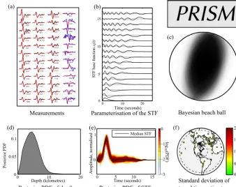
In a companion paper (Stähler and Sigloch, 2014), we developed the PRobabilistic Interference of Source Mech-anisms (PRISM) algorithm, a fully probabilistic inversion for source depth, moment tensor and STF, via sampling by both stages of the neighbourhood algorithm (NA; Sambridge, 1999). Figure 1 sums up the procedure and its results.
The need for PRISM arose from our work in global-scale waveform tomography, which fits broadband body-wave seismograms of moderate to large earthquakes to mod-elled synthetics, up to the highest occurring frequencies
(≈ 1 Hz). This can only be achieved with good a priori es-timates of source depth, which strongly shapes the synthetic Green’s functions, and of source time functions, which con-volve the Green’s functions. At the time, no data centre de-livered routine estimates of broadband STFs (by now, efforts other than ours are underway; Vallée et al., 2011; Vallée and Douet, 2016). Hence Sigloch and Nolet (2006) developed a linearised, iterative approach that semi-automatically de-convolved broadband source time functions, source depths and moments tensors of more than 2000 earthquakes, which were subsequently used in several waveform tomographies (Sigloch et al., 2008; Sigloch, 2011; Sigloch and Mihalynuk, 2013; Hosseini and Sigloch, 2015).
The required human supervision time called for full au-tomatisation, preferably in a Bayesian setting that would cir-cumvent the occasional divergence of the non-linear optimi-sation and would automatically diagnose parameter trade-offs of the kind described. PRISM (Stähler and Sigloch, 2014) solved this problem, but we left the justification of its misfit criterion and the derivation of its noise model and like-lihood function to the present study.
Measurements Parameterisation of the STF
(f.)
(b) (a)
Depth (kilometres)
Posterior PDF
Time (seconds) Standard deviation of travel time estimate
(d) (e)
c
Bayesian beach ball
log
10
(PDF)
0 0.5 1.0 1.5 2.0 Time (seconds)
(c)
0 0.05 0.1
0 10 20 0 10
0 1
seconds
Posterior PDF of STF
5 15
Posterior PDF of depth
A
m
pl
it
ud
e,
n
or
m
al
ise
d
Figure 1. Visual summary of the fully probabilistic source inversion algorithm PRISM presented in the companion paper (Stähler and Sigloch, 2014), on the example of a magnitude-5.7 earthquake in the US state of Virginia on 23 August 2011.(a)Candidate source so-lutions are evaluated according to the cross-correlation fit they produce between observed broadband, teleseismicP waveforms (black) or SHwaveforms (blue), and their modelled counterparts (red). The present study is concerned with quantifying the noise distribution on these
cross-correlation measurements CC – one scalar per source–receiver pair, 48 in total for this earthquake.(b)To reduce the dimensionality of the model space to a number accessible to Bayesian sampling, the source time function (STF) is parameterised as a linear combination of 15 empirical orthogonal functions found to best span the space of a large set of 900 reference STFs (Sigloch and Nolet, 2006; Stähler and Sigloch, 2014).(c)The “Bayesian beach ball”, a visual average of the posterior ensemble of well-fitting solutions, conveys not only the nature of the moment tensor but also the magnitude and nature of its uncertainties.(d)The marginal probability of the hypocentre depth. (e)Weighted average of STFs from the posterior ensemble of good solutions permits assessment of the uncertainties in STF shape. This STF is clearly unimodal and of less than 5 s duration.(f)As a secondary benefit, this procedure yields the uncertainties (standard deviations) of cross-correlation travel time measurements at all stations, and their inter-station correlations. Travel times are the primary input data for seismic tomography, and these insights into their uncertainties are not readily available from other methods.
space has to be as small as possible, preferably less than 20. Depth is one parameter, and a normalised description of the moment tensor requires five more (a more rigorous and uni-form parameterisation of the moment tensor has been derived by Tape and Tape, 2015, 2016). Although latitude and longi-tude could easily be added to this list, we do not consider them here, because the lateral location problem is adequately addressed by existing data centres (National Earthquake In-formation Center (NEIC) or Bondár and Storchak, 2011), and in any case we would re-estimate all hypocentres at the time of tomographic inversion. The STF is a high-dimensional pa-rameter vector, which Sigloch and Nolet (2006) and Stäh-ler et al. (2012) parameterised simply as a time series of 256 unknowns (10 Hz sampling rate, 25.6 s length). To re-duce its dimensionality for Bayesian sampling, Stähler and Sigloch (2014) made use of a dataset of >2000
determin-istic earthquake source solutions (depth, moment tensor and
STF) obtained by Sigloch and Nolet (2006). We selected the 900 best-constrained STFs and composed this set into empir-ical orthogonal functions (EOFs), denotedsl(t ). Any
broad-band STFs(t ) of events up to magnitudes of about 7.5 is
well described by a linear combination of the firstLEOFs,
whereL≈15 delivers sufficient accuracy for our purpose:
s(t )=P15
l=1alsl(t ). These EOFssl(t ), shown in Fig. 1b, are the primary means by which we feed a priori expert knowl-edge into the Bayesian sampling problem. PRISM’s STF pa-rameterisation consists of the firstLEOF weightsal,
beach ball” plots (Fig. 1c), a superposition of many beach ball representations in the a posteriori ensemble. A valuable side benefit is full uncertainties on travel time measurements
1Tj at stationsj. These travel time delays are incidental in the context of source inversion (as the time shifts between ob-served and synthetic seismograms that maximise the cross-correlation coefficients CCj, Fig. 1f), but they represent the primary input data for our seismic waveform tomographies.
The primary measure of fit (or “input data”) for PRISM’s source inversions is the CCj. When parameter estimation is performed as a deterministic optimisation problem, (only) a relative measure of fit or misfit is required: the optimal solu-tion is the one that yields the smallest misfit between obser-vations and model predictions, in our case the largest possi-ble values of cross-correlation coefficients CCj. By contrast, Bayesian parameter estimation requires not just a measure of misfit but also a likelihood function for it, which is de-rived from the probability distribution on the data (the “noise model”). In the absence of a noise model, the likelihood of a randomly drawn candidate solution cannot be evaluated. Obtaining a noise model for a misfit requires much more in-formation about the measurement process and its statistics than the mere adoption of a misfit measure. This is the big challenge of Bayesian “inversion”, which will be covered in this paper.
Section 2 argues for the adoption of the signal decorrela-tionD=1−CC as a robust measure of misfit, where CC is the normalised cross-correlation coefficient (Table 1). To our knowledge, the decorrelationDof seismological waveforms
has not been used as a misfit criterion in Bayesian inference (other than by Stähler and Sigloch, 2014) because its noise model and likelihood function were unknown – a shortcom-ing D shared with other deterministic misfit choices, such
as the instantaneous phase coherence (Schimmel, 1999), time phase misfits (Kristekova et al., 2006) or multi-tapers (Tape et al., 2009).
Section 2.2 shows that the popular`2and`1norms
(Maha-lanobis, 1936) would be sub-optimal misfit criteria because noise in seismic signals is not simply additive Gaussian or Laplacian but rather partly signal-generated, i.e. highly cor-related across time samples and stations, and better described by a transfer function. Figure 2 shows an example of this systematic noise “coda”. Section 2.3 defines the general re-quirements of a good misfit criterion, and Sect. 2.4 demon-strates that the signal decorrelation D performs more
ro-bustly than sample-by-sample (`p) norms on realistic
seis-mological waveform data.
To identify a likelihood function L(m|d) of misfitD in
Sect. 3, we draw once more on the prior knowledge con-tained in our set of deterministic source solutions for 900 earthquakes and on the 200 000 measurements of CC=1−D
made to obtain them. From this large, representative and highly quality-controlled dataset of confident source solu-tions, we obtain the statistics of the residual misfitsD, which
we use to construct an empirical likelihood L∗(m|d). Thus
High SNR, good fit
High SNR, poor fit
Low SNR
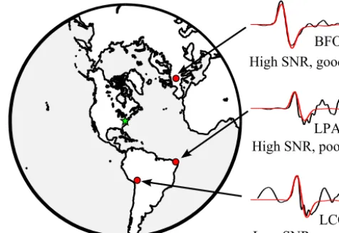
Figure 2.Three noise cases for compressional (P) waves in source
inversion; the waveforms were produced by the M 5.7 earthquake in Virginia (23 August 2011). Station BFO has a high signal-to-noise ratio (no wiggles preceding theP pulse), and the waveform
is fit well by a WKBJ synthetic using our best source solution for this earthquake. Station LPAZ has a high signal-to-noise ratio, but 3-D structure produces a strong coda following theP pulse, i.e.
signal-generated, systematic “noise” not fit by the synthetic wave-form. Station LCO has a low signal-to-noise ratio and a coda. Since the coda cannot be modelled, it must be considered noise, albeit of a systematic nature and correlated across time samples and across stations. By contrast, ambient noise is random and not correlated across stations, only across time samples (since the signal is band-limited).
we can instruct the probabilistic inversion to explore sub-spaces of solutionsmthat yield similarly low levels of misfit Das these best-fitting deterministic solutions.
Section 3.6 presents a worked example for the construction of a likelihood functionL(m|d)from data of a typical
earth-quake, the 2011 Virginia event used throughout this paper and its companion Stähler and Sigloch (2014). We conclude with a discussion in Sect. 4.
2 Noise and misfit criteria 2.1 Bayesian inference
Bayesian inference estimates the posterior distributionπ(m)
of the parameters m given d, using the prior distribution p(m)of the model parametersmand the likelihoodL(m|d)
of the datad, given the modelm, by applying Bayes’ rule:
π(m|d)= 1
p(d)L(m|d)p(m). (1)
p(d)is the prior distribution of the datadand does not de-pend on the experiment. A likelihood function L(m|d) is
pre-dicted datag(m). This difference or misfit is defined,
follow-ing convention, as
8(d, g(m))= −ln(L(m|d)), (2)
so that a model with a high likelihood has a diminishing mis-fit. Since the likelihood of a model can vary by orders of magnitude, the logarithm brings the misfit back to natural scaling.
The exact formula for L(m|d) depends on the assumed
noise model and potential error sources in the forward model. Equation (2) requires that the misfit criterion take those into account as well. Next, we will show that this is straightfor-ward only for specific assumptions about the noise, which are usually not realistic.
2.2 Metric-based misfit criteria
“Good” solutions m are associated with small misfits 8,
where the exact definition of 8 depends on the nature of
the datad, which may be hand-picked arrival times; disper-sion curves; or, in our case, seismic displacement time series (“waveforms”). A waveform misfit is generally a functional
8W :RN×RN7−→ [0,∞)ond,g(m)∈RN.
The misfit functional has similar properties to a metric on RN, but it should be noted that there is no natural choice; rather, its choice implies a strong assumption of prior knowl-edge about the statistical properties of the noise ond. In the case of seismic waveform data, the data vectordis the mea-sured time-sampled seismogramui and the separate data are the samplesui, i= {1, . . ., n}of this time series. The vector g(m)is the synthetic seismogramuci, i= {1, . . ., n}predicted by the forward operatorgfor the modelm.
When the method of least squares is used to calculate the
`2misfit, 8W
`2(m|d)=k 0
1
2(d−g(m))TS −1
D (d−g(m))
, (3)
the assumption is that the noiseis additive and Gaussian-distributed:
d=g(m)+, ∼N(0,SD). (4)
The size [N×N] data covariance matrix SD∈SymN de-scribes the correlation between the error of individual mea-surementsdi.k0is a normalisation constant.
In the case of a seismic waveformui,8W is
8W
`2(m|d)=k 0
n X
i=1 n X
i0=1
(ui−uci)T(S −1
D )i,i0(ui0−uci0), (5)
andSD describes mainly the band-limited spectrum of en-vironmental noise. Since a simple time shifting ofui or uci will violate the assumption of Eq. (4), the ui oruci need to be aligned first. Because we assume this noise to be time-invariant, we can buildSDfrom the autocorrelation function
R of the (discrete) noise time seriesi. SD is a Toeplitz matrix, where the rows are shifted instances of the autocor-relation functionR.
SD,k,k+l=R(l)= n X
i
ii−l (6)
See Bodin et al. (2012) for an example of how to construct SD under the assumption of an autoregressive (AR) noise model.
For the estimation of the parametersmof one earthquake source, we would normally use seismograms measured at different stations, cut into a total ofnS time windows ui, counted with indexj. The overall misfit8(m)for a source
solution will be comprised of the misfits of the single wave-forms8W
`2,j(m). If the noise on each waveformjis assumed to be uncorrelated with the noise on all others, then it is le-gitimate to define the overall misfit as being simply additive:
8(m)= nS X
j=1
8W`2,j(m). (7)
If the noise on the waveforms is correlated, then Eq. (3) has to be extended, such thatd,mandSDcontain all time sam-ples of all waveforms recorded at different stations. This ef-fort has – to our best knowledge – not been made in seismic inverse problems.
If each measurement i is considered to be uncorrelated
with the others and has a varianceσi, thenSDis a diagonal matrix with diagonal elementsσi2and Eq. (3) reduces to
8W
`2(m|d)=
k0
2 N X
i=1
(di−gi(m))2
σi2 (8)
or, in the case of waveforms,
8W`2(m|d)=
k0
2 N X
i=1
(ui−uci)2
σi2 . (9)
With a set ofnS waveformsui,j, the total misfit defined in Eq. (7) becomes
8=k 0 2
nS
X
j=1 nj
X
i=1
(ui,j−uci,j)2
σi2 , (10)
the weighted least-squares criterion.
If the noise can be described well by the normal distribu-tion, the`2norm can be successfully applied. It is, however
Hence, Käufl et al. (2013) have proposed to use the more outlier-resistant`1norm as a misfit criterion of observed and
modelled seismograms. They assume that noise on the time samplesui is independently Laplace-distributed with width
bi, i.e. no temporal correlation:
d=g(m)+, i∼Laplace(0, bi), (11)
8W
`1(m|d)= − X
i
|di−gi(m)|
bi
−ln2bi. (12)
Time samples of realistic, band-limited seismograms are strongly correlated, which calls for the use of multivariate Laplace distributions. This is the subject of ongoing research (Kotz et al., 2001; Kozubowski et al., 2013), but the resulting probability density functions (PDFs) are still too complex to be used in ensemble inference. To make things worse, seis-mograms recorded at different stationsj will generally also
be correlated. Hence the simplicity of the univariate Laplace distribution is not applicable, and the robustness of the `1
norm currently cannot be harnessed.
Other authors have proposed to use misfits based on gen-eral`pnorms (e.g.p=1.5 in Sambridge and Kennett, 2001),
which allow the robustness of the misfit to be tuned to the noise on the data.
8W`p(m|d)=
n X
i=1
|di−gi(m)|p
σp
!1/p
(13)
The underlying noise model is an exponential power distribu-tion. However, all problems described for the`1norm apply
here as well, and no multivariate forms exist in general. In summary, it is tempting to chose `p misfits based on
the time-sample-wise distance between observed and mod-elled waveforms because the underlying noise models are straightforward to state (uncorrelated or correlated Gaussian, uncorrelated Laplace distribution) and to translate into cor-responding likelihood functions. Unfortunately, these noise models are very crude approximations of the pervasive noise characteristics and correlation found in real time series.
These serious shortcomings motivate our proposal of al-ternate misfit criteria.
2.3 Noise-model-based misfit
In a Bayesian context, the likelihoodL(m|d)is a defined by
the noise model on the data. An equivalent functionL∗(m|d) can be constructed from the distribution p(F )of any
func-tional F of the observed and predicted waveformsui,uci ∈ R:F:R×R7−→ [0,∞). In our attempt to move beyondF
being a sample-wise distance betweenui anduci, we gener-ally want a candidateF to meet the following conditions:
1. Forui=uci,F should take a fixed value, say 0.
2. With decreasing similarity ofui anduci,F should in-crease, irrespective of the exact definition of similarity (Sect. 3 will consider this further).
3. F should be robust against time shifts 1t=k·dt or
amplitude errors a affecting the waveform ui, i.e.
F a·ui+k,uciuF ui,uci for any a∈R, k∈N, be-cause such unknown time shifts will affect real-world seismograms.
4. F should have discriminative power with respect to the
model parametersm, combined with robustness against realistic noise and theoretical errors.
Concerning the noise, we need to be able to calculate the distribution ofF for a waveform afflicted by the typical three
error sources: background noise, waveform modelling error and instrument error.
1. Ambient noisenoise: this is noise from man-made or natural sources around the receiver. It can be described very well by an additional term, likenoise∼N(0,S)
(see Eq. 5).
2. Waveform modelling errorTmodel,i: the synthetic wave-formuci can never be identical to the observedui, even in the absence of ambient noise. In the context of source modelling, the earth’s impulse response (Green’s func-tion) can be considered a linear, time-invariant opera-tor that acts on the source time function. The calcu-lation of this Green’s function is not perfect (e.g. due to errors in the earth model or imperfect computational methods). Tarantola and Valette (1982) called this the theoretical density function and proposed to model this systematic error by an additive term onuci, but we think that it should rather take the form of a transfer function Tmodel,i, between ui anduci, which will hopefully be Dirac-like in character. However,Tmodel,i will include the site response (receiver side reverberations), which can create strong waveform coda; see Fig. 2. Hence, Tmodel,i could in practice be rather oscillatory.
3. Instrument errorTinst,i: a displacement seismogramui is assumed to have been corrected for the instrument response of its seismic sensor. In practice, this correc-tion may be imperfect (Bogert, 1962), e.g. due to roneous sensor metadata. We model this systematic er-ror by another (hopefully Dirac-like) transfer function Tinst,i convolvingui.
In summary, the difference between a modelleduci and ob-served waveformuiis
ui=uci∗Tmodel,i∗Tinst,i+noise,i. (14)
It is this complex mixture of noises that misfit criterion
F should be robust against while retaining discriminatory
power toward source model parametersm.
Next, we will test the signal decorrelationDas an
2.4 Signal decorrelation coefficient as a misfit
We choose the signal decorrelation D as a misfit criterion,
defined as
Dui,uci =1−max k
{CCui,u
c i
k }, (15)
where CCui,uci
k =
Pn
i=1 wiuci−k·ui
q
Pn
i=1(wiuci−k)2·
Pn
i=1(wiui)2
(16)
is the normalised cross-correlation coefficient and k is the
time delay between uci and ui for which the normalised cross-correlation function CCui,uci
k takes its maximum value. wi is a window function that allows to select a time window for the cross-correlation measurement. D satisfies three of
the four criteria that we desired of a misfit in the last section: 1. Dui,uci takes the value 0 for identical signalsuc
i ≡ui, since CCui,uci
k=0 =1. 2. Forui6=uci,0< Dui,u
c
i <2, i.e.Dvalues larger than
for the caseuci ≡ui, andDui,u
c
iincreases with
decreas-ing similarity ofui anduci.
3. If a time shift k0 is small compared to the window
length, we have CCui,uci
k ≈CC
ui,uci+k0
k+k0 and thusDui,u c
i ≈Dui,uci+k0 .
Due to the normalisation in Eq. (16),D is
amplitude-independent:
CCui,uci=CCui, a·uci and thusDui,uci =Dui, a·uci
The fourth criterion, discriminative power and robustness against noise is less straightforward to demonstrate. We pro-ceed empirically by showing its superior performance over the`2and`1misfits on an example of the kind of waveforms
we typically use for source inversion. Figure 3 shows in black a simulated, broadband, noise-freePwave train, recorded at
40◦epicentral distance. The seismograms were modelled us-ing the WKBJ method of Chapman (1978) in the IASP91 ve-locity model (Kennett and Engdahl, 1991), assuming an ex-plosion source withM0=1020Nm. Since the chosen source depth is shallow (10 km), thePpulse is followed within
sec-onds by depth phases likepP, which effectively permits
in-version for source depth. However, once this waveform gets perturbed by realistic modelling error (convolutive) and addi-tive noise, resulting in the red waveform, the fit to the unper-turbed original becomes tedious. A meaningful robustness test is as follows: if the perturbed (red) waveform is mod-elled for different candidate source depths, will the smallest misfit be achieved for the perturbed wave simulated at the correct depth of 10 km? This is a meaningful test of robust-ness, because source depth tends to be the most challenging parameter to retrieve in source inversions. Algorithmically, the perturbation is done in two steps:
1. Perturbation by convolution with a “modelling er-ror function” Terror,i, which encompasses effects of Tmodel,i andTinst,i. It is defined as having a unit ampli-tude spectrum and a random phase spectrum between 0 andα·π/2.
um.e.=uci∗Terror,i (17) This method adds realistic coda to the waveform, which simulates the effects of structure, that was not included in the forward simulation. The parameterαregulates the
perturbing effect of the modelling error function. 2. By adding a band-limited noise term
upert=um.e.+β,where∼N(0,SD), (18) the covariance matrixSDis set to model a band-limited noise with corner frequencies of(1/15,1/6 Hz), similar
to microseismic background noise at the seismic station. The peak amplitude is normalised to that ofuci, so that the parameterβ controls the relative amplitude of this
noise term.
Figure 3 shows the resulting reference waveform (left) and perturbed waveforms forα=0.4 andβ=0.8, i.e. moderate
perturbation of the signal and strong background noise. The unperturbed waveformui is plotted in solid, thin black, the waveform perturbed with modelling errorum.e.in dotted blue and the resulting reference trace in solid red. It bears little resemblance to the unperturbed waveform.
The right plot shows the value of the three waveform mis-fits`1,`2andDbetweenuci andupert over varying source depths. It simulates an inversion for the depth of an earth-quake using seismic waveforms. The waveform contains the
PandpParrival. The depth is mainly constrained by the
rela-tive arrival time of the three and the resulting waveform of the wholeP−pPwave train. The perturbation of Eq. (18) adds
artificial coda with additional arrivals to the waveform, which a good waveform misfit should be robust against. The misfit should have a distinctively lower value for the “true” depth of 10 km than for any of the others. To take into account the stochastic nature of these perturbations, 500 realisations of upertwere calculated for the same parameters,αandβ, but
with different random numbers. The coloured shades mark the 95 % (2σ) quantiles of the misfit values; the solid line
marks the median.
The`2misfit could not recogniseuci inupertanymore and assigns the lowest misfit to a depth of 3 km. An analysis of different noise and perturbation levels shows that the`2norm
is relatively robust against background noise, but not against perturbations from a modelling error; see Fig. S1 in the Sup-plement. This seems reasonable given the underlying noise model of this misfit.
The`1norm does better, in that it has a minimum at 9 km
0 5 10 15 20 25 30 0
0.5 1 1.5
D epth / km
Misfit value
Misfits for = 0.4, = 0.8
² ¹
D
2confidence interval Median value
0 5 10 15 20 25
1 0.5 0 0.5 1
Amplitude, normalised
T ime / s
Pure reference trace
Waveforms for= 0.4,= 0.8
wave
wave
D
isturbed ref. trace D
ist. ref. trace + noise
T rue depth
P
pP
Figure 3.Comparison of the`1, `2norm and the signal decorrelationComparison of the`1, `2norm and the signal decorrelationD=1−CC
as misfit criteria in noisy signals. A perturbed synthetic waveformucpertfor a 10 km deep explosion source, measured at a station at 40◦
epicentral distance, was compared to synthetic seismogramsuc for other depths, using the three misfit criteria. The shaded colours mark
the 95 % quantiles of the misfit values, calculated by perturbing the reference waveform with different random seeds. The figure shows the relatively high robustness of the cross-correlation coefficient in recognising reference signals in perturbed measurements. For better visualisation, all misfit values have been normalised separately to have an average values of 1 between 20 and 30 km.
0 5 10 15 20 25
5σ 10σ 15σ
Signal-to-noise ratio Misfit value for true depth 12σσ
ℓ², weak pert. D, weak pert.
ℓ¹, weak pert.
D, strong pert. ℓ², strong pert. ℓ¹, strong pert.
Figure 4.Distance between misfit value for the true source depth vs. the plateau for depths 20–30 km in standard deviations. See Fig. 3 for waveforms and misfit curves. The “weak-perturbation” curve is calculated with perturbation factor α=0.1, and the
“strong-perturbation” curve withα=0.9 (see Eq. 17). For all SNR values,
the decorrelation has a higher discriminative power than`1or`2.
at 9 to 10 km reaches only slightly below the lower quartile for other depths, meaning that in reality the resolution power of the`1norm for this kind of problem will be very limited.
The studies for different noise and perturbation levels show that it is generally more robust against background noise and modelling error than the`2norm but less so than the
cross-correlation coefficient.
The cross-correlation misfit has the strongest difference between the plateau of wrong depth solutions and the true one. For low noise levels, the minimum is slightly wider than the one for the`1norm. More values ofαandβ are shown
in Fig. S1. The analysis of the confidence intervals shows that the values for CC scatter slightly more than the ones for
`2and much more than for`1. To employ it in Bayesian
in-ference, a detailed analysis of the statistical properties will be necessary. The analysis also shows that the actual values ofDare influenced more strongly by the background noise
level than by the modelling error. We will use that observa-tion in Sect. 3.3.
Figure 4 compares the resolution power of the three mis-fits for different perturbation levels and signal-to-noise ra-tios (SNRs). It shows the difference between the misfit value for the true depth 10 km and the average misfit value for the depths between 20 and 30 km. The difference is expressed in numbers of standard deviations (sigmas) from the 500 sepa-rate noise realisations. The dashed line shows the result for weak perturbation (α=0.1), and the solid line for strong
per-turbation (α=0.9). It can be seen that, for strongly perturbed
waveforms, the `1 and `2 norm cannot recognise the true
depth with more than 2σ, even for high signal-to-noise
ra-tios, while the decorrelationDstays well above 3σ, even for
SNRs of 6.
3 Empirical likelihood function for the signal decorrelation
3.1 Empirical likelihood function obtained from high-quality, deterministic source estimates
In seismology, the cross-correlation coefficient CC=1−D
0 0.2 0.4 0.6 0.8 1 0
0.02 0.04 0.06 0.08 0.1
Decorrelation
p
S amples Beta distr. Exponential distr. Logn. distr.
10−2 10−1 10−2
10−1
Data quantiles
Distributions’ quantiles
45°line Beta distr. Exponential distr. Logn. distr.
( a)
( b)
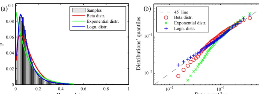
Figure 5.Probability distribution ofD, the decorrelation of measured and syntheticP waveforms used for deterministic source inversions. (a)Empirical histogram ofDis shown as grey bars. From 200 000 broadband, teleseismicPwaveforms for 900 earthquakes, only waveforms
with signal-to-noise ratios between 20.0 and 21.0 were considered for this figure (because the scaling parameters of analytic fitting functions depend mainly on SNR). Coloured lines show best-fitting realisations of three analytic probability density distributions: beta (red), exponen-tial (green) and log-normal (blue). The log-normal distribution yields the best fit to data.(b)Quantile–quantile plot for the three candidate distributions of(a)confirms that the log-normal distribution best fits the empirical histogram ofD. The values on thexaxis are percentiles
of the cumulative histogram ofDin our dataset. Theyaxis shows the percentiles of the best-fitting distribution of each class. The closer the
percentiles are to the liney=x, the better the fit of the distribution to the underlying data over the entire range of values. Both subfigures
indicate that a log-normal distribution best fits the values ofD=1−CC.
only aware of Kikuchi and Kanamori (1991) and Marson-Pidgeon and Kennett (2000). CC andD=1−CC have not been used in probabilistic inversion, and the main obstacle would have been their unknown statistics.
We present an empirical solution to this problem by draw-ing on a large, pre-existdraw-ing database of cross-correlation measurements that we assembled in the context of determin-istic source inversions, as described in Section 1. Essentially we assert that our human expert knowledge and extensive experience have generated a large, representative and highly quality-controlled set of 900 teleseismic source parameter es-timates that are sufficiently close to the true source parame-ters to reveal the statistics of the noise in the measurements d these estimates mare based upon. The measurements d consisted of 200 000 cross-correlation coefficients CC ob-tained from 200 000 broadband fits of observed seismograms to WKBJ synthetics. The synthetic waveforms were calcu-lated using the WKBJ method (Chapman, 1978) in velocity model IASP91 (Kennett and Engdahl, 1991), with attenua-tion and density taken from PREM (Dziewo´nski and An-derson, 1981). To the extent that our source solutions mj approach the true source parametersm0,j, the histogram of the CC (orD=1−CC) values approximate the probability density function of CC (or D) in the presence of noise and
modelling errors. Thus we can obtain an “empirical likeli-hood function” L∗(m|d)even in the absence of an analyt-ically describable noise model. We preface the term “like-lihood” by “empirical” because strictly speaking the likeli-hood would be associated with the noise model on the raw samplesi, rather than with the noise on the composite
mea-sureD. A similar approach has been adopted independently
and recently by Bodin et al. (2016) in the context of receiver-function inversion. Note that the term “empirical likelihood” has been used differently in statistics (Owen, 1988).
Our reasoning and procedure can be summed up as fol-lows:
– We can consider the measurements of misfit functional
8j(m0|d)for one earthquake atj=1, . . ., nSrecording receivers as realisations of a random process that fol-lows a yet unknown probability density functionp(x). m0are the true source parameters, and any misfit8j is therefore due to ambient noise and modelling errors in the seismograms, as described in section 2.3.
– In practice we never get to knowm0but only a (hope-fully close) estimatemest, the result of a deterministic source inversion procedure. Hence all we can actually observe is8(mest|d), some of which is due to the
es-timation errormest−m0. However, by estimatingmest carefully and repeatedly (for 900 different earthquakes), and by considering the resulting 900 sets of misfits8
(at 200 000 source–receiver pairs) jointly, the histogram of their 200 000 D values should approximate a
his-togram of the true8(m0|d)as closely as we can hope
to get. Figure 5a shows this empirically obtained his-togram8cumulativeofDin grey (for the subset of P
seis-mograms that had a SNR of 20; reason to be discussed). – To evaluate the likelihood of a misfit value80
encoun-tered in a future (Bayesian) inversion, we could in prin-ciple compare it to this empirical histogram8cumulative.
thep(x)that produced this histogram8cumulativeand to evaluate any80against thisp(x).
– The best we can do is to identify a suitable type of distri-bution and fit its parameters to the empirical histogram
8cumulative of Fig. 5a, thus obtaining a PDF pfit(x)as
our best estimate for the truep(x).
– The likelihood of a data vectordgiven modelmis then considered to be
L∗
(m|d)=pfit(8(d|m)) . (19)
3.2 Approximate log-normal distribution of decorrelationD
We will consider three candidate distributions for fitting an analyticpfit(x): beta, exponential and log-normal. They are
all positive one-sided (defined only forD >0) and can take
negligible values forD >2, where strictly they should be 0.
Figure 5a shows their fits to the empirical histogram after determining the best-fitting scale parameters for each.
The beta and the exponential distributions are seen to over-estimate the number of very small D values (i.e. values of
CC≈1). Hence these distributions would predict more ex-cellent waveform fits than observed. The likelihood of actu-ally well-fitting waveforms would be estimated too low; i.e. we would be too pessimistic about the achievability of good waveform fits.
The log-normal distribution clearly yields the best ap-proximation of the D histogram. This is confirmed by the
quantile–quantile plot of Fig. 5b. Hence we choose the log-normal distribution to express our likelihood function.
The (univariate) log-normal distribution function is de-fined by two scale parametersµandσ:
f (x)= 1
x
√
2π σ2exp
−(lnx−µ) 2 2σ2
. (20)
The log-normal distribution also yields the best fit to our synthetic data from Sect. 2.4, as calculated with the perturba-tions in Eqs. (17) and (18). See Fig. S4 for a corresponding quantile–quantile plot.
If random variablexin Eq. (20) is equated with the
decor-relationDj of one waveformj, the logarithm ln(Dj)is nor-mally distributed with meanµand standard deviationσ. This
fortunate link of our empiricalDhistogram to the Gaussian
distribution makes it trivial to express the joint, multivariate distribution of all nS waveform measurements of an earth-quake, collecting the Dj in vector D and the inter-station covariances innS×nScovariance matrixSD.
ThenS-variate likelihood function forDbecomes
L∗ D=
exp−12(ln(D)−µ)TS−D1(ln(D)−µ)
(2π )n2
√
|det(SD)|
, (21)
10
20
300 0.2 0.4 0.6 0
0.02 0.04 0.06 0.08 0.1
Decorrelation
Signal-to-noise-ratio
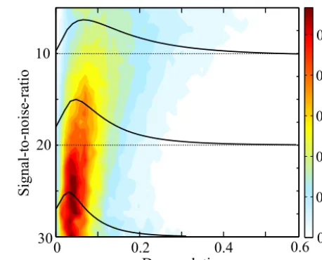
Figure 6.Colour shade map out a two-dimensional histogram of waveform decorrelationD, as a function of waveform SNR along
theyaxis. All 200 000 waveform measurements from our 900
de-terministic source inversions entered this histogram. Black lines are the best-fitting log-normal distributions for SNRs of 10, 20 and 30. (The 1-D histogram for SNR=20 was discussed in Fig. 5.) Toward
smaller SNRs (high-noise conditions), theD distribution widens
(more occurrences of poorly fitting waveforms).
and the misfit becomes
8 = 1
2 n X
j=1 n X
k=1
ln(Dj)−µjT(SD−1)j k(ln(Dk)−µk) !
+ 1
2ln (2π ) n|det(S
D)|
. (22)
This is the Mahalanobis distance, not between the individ-ual samples of two waveformsui anduci as in Eq. (3) but between the decorrelationDj of these two waveforms and its expected valueµj, taking into account correlated noise between two stations inSD.
Thus the use ofDas a misfit criterion reduces the number
of misfit values tonS per earthquake (the number of source
receiver paths, or waveforms) compared toPnS
j=1nj in the case of the`1or`2norms (nj is the number of samples on waveformj). In other words,Djitself accounts for any cor-relations across time samples on seismogramjand subsumes
them into a single number, leaving only spatial (inter-station) correlations to be dealt with inSDand in the empirical like-lihood functionL∗.
3.3 Distribution coefficients determined by signal-to-noise-ratio
Here we describe howµ andSD can be estimated for one earthquake. So far it was implicitly assumed that a single distributionpfit might fit8cumulative for all source–receiver
This may be an oversimplification since ambient noise lev-els noise show significant diurnal and seasonal variations, and are elevated at stations close to coastlines or cities (Peter-son, 1993; Stutzmann et al., 2009). Hence we might expect goodness of fit to vary across stations, which could be mod-elled by adjusting the scale parameters of the log-normal dis-tribution for each station. Goodness of fit is also influenced by earthquake magnitude, and by station distance and back azimuth, so we might even require different scale parameters for each source–receiver pair.
To avoid this level of complexity, recall the investigation of Sect. 2.3 that revealed the distribution of D to be most
sensitive to the level of ambient noisenoise. Hence we bin
our 200 000 source–receiver pairs by SNR and estimate only one pair of (µ, σ) distribution parameters per SNR bin. This
hopefully subsumes all individual sources of random misfit. SNR is defined as the integrated spectral energy in the sig-nal time window, divided by that of a 120 s noise window prior to the arrival of the first body-wave energy. Signal time windowsui, i=1, . . ., Nsignalare as follows: forPphase, 5 s before to 20.6 s after its theoretical arrival time in IASP91, on theZcomponent; forSHphase, 10 s before to 41.2 s after, on
the T component. Noise time windows ni, i=1, . . ., Nnoise are as follows: for bothPandSHphases,−150 to−30 s be-fore theoretical arrival time. We calculate SNRs forP and SHwaves as
SNR=Nnoise PNsignal
i=1 u2i
NsignalPNnoise
i=1 n2i
. (23)
Note that this way the noise window of the P wave
mea-surement contains only ambient noise, whereas theSHwave
noise window is in addition afflicted by some signal-generated noise:P coda and phases like PPorPcP, which
get scattered into the transverse component due to lateral het-erogeneities and anisotropy in the real earth.
Figure 6 shows theDhistogram and three fitted
probabil-ity densitiespfit(D), as a function of SNR. Under low-noise
conditions (high SNR), the log-normal distributions are nar-rower and centred on smallerD misfit values, which seems
plausible.
By fitting functions of the formh(SNR)=a1+a2·exp(a3· SNR)to the SNR-binnedDhistograms, we determined
dis-tribution parameters µP(SNR), µSH(SNR), σP(SNR) and
σSH(SNR)for SNR ranging from 1 to 1000 forP waveforms and from 1 to 200 for SH waveforms (see Supplement for
details).
Hence the log-normal distribution pfit(D) ascribed to a
given source–receiver pair depends only on the ambient signal-to-noise ratio of the receiver i, and its scale
param-eters are given by
µi =aµ,1+aµ,2·exp(aµ,3·SNRi), (24)
σi =aσ,1+aσ,2·exp(aσ,3·SNRi). (25)
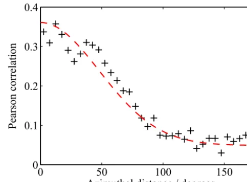
0 50 100 150
0 0.1 0.2 0.3 0.4
Pearson correlation
Azimuthal distance / degrees
Figure 7.Correlation in misfit between neighbouring stations. The measured Pearson correlation (see Eq. 26) is plotted over the differ-ence in azimuths between two station for the same earthquake. A fit functiongb1,b2,b3(ϑ )=b1+b2·exp(−b3ϑ2)is plotted in dashed
red lines.
The exact values for ai depend on the velocity model and the solution method. Here, we used the WKBJ method, which results in a simplistic crustal response. Other meth-ods, like the spectral-element method, in combination with a waveform database (as implemented in Instaseis by van Driel et al., 2015) may produce more realistic seismograms, result-ing in higher average values ofD. What matters is that the
actual inversion uses exactly the same solver and velocity model as was used to determine the distributions ofD.
3.4 Estimating inter-station covariances
Decorrelation values D measured at different stations
can-not be expected to be uncorrelated, because systematic mod-elling errors (due to differences between assumed earth model and true earth, and to methodical inadequacies in the Green’s function computations) will affect neighbouring sta-tions in similar ways. A reasonable guess is that stasta-tions at similar azimuths from the source would show the strongest correlations because their wave paths have sampled similar parts of the sub-surface, in particular similar parts of the crust and upper mantle – regions to which the strongest modelling errors can be ascribed.
To check these systematics, we calculated the Pearson cor-relation coefficientr(ϑ )as a function of azimuthal distance ϑ as follows. For each earthquake, we calculated the
az-imuthal distances ϑj k between all station pairs (j, k) and binned those. A set{j, k}ϑthen contains all stations pairs for one event that have the same azimuthal distanceϑ(in bins of
5◦width).
We need to adjust for the fact that stationsj andk
standard score of each stationj as zj= ln(Dj)−µj/σj and from this the Pearson correlation coefficient of aϑ bin
{j, k}ϑ, using allnϑstation pairs in that bin:
r(ϑ )= 1
nϑ−1 X
{j,k}ϑ
zjzk. (26)
The use of standard scores permits comparison of stations of different SNR and hence log-normal distribution parameters. The values forr(ϑ )are then fit by a function (see Fig. 7)
g(ϑ )=b1+b2·exp(−b3ϑ2). (27)
This permits comparison ofDj for stations with different SNR and distributions ofDj. Then the correlation coefficient was calculated for each azimuthal bin ϑ using all nϑ pairs {i, j}ϑin this bin.
This azimuth-dependent correlation coefficient g(ϑ )can
be used to fill the elements of covariance matrix SD in Eq. (21):
SD,i,j=
σiσj· b1+b2·exp(−b3ϑ2), i6=j
σi2, i=j. (28)
An example of such a covariance matrix is shown in Fig. 8. It is for the 2011 earthquake in the US state of Virginia that was used as a detailed working example of Bayesian source inversion in the companion paper (Stähler and Sigloch, 2014).
3.5 Misfit distribution of waveform amplitude measurements
Waveform amplitudes have not been considered so far, even though they provide crucial constraints on focal mechanisms. Our amplitude measurement consists of a comparison of the logarithmic energy content ln(A)in a 1 s time window
around the peak i=i1, . . ., i2 of the measured seismogram
and its synthetic:
1ln(A)j=ln i2
X
i=i1
u2j,i !
−ln i2
X
i=i1
ucj,i2 !
. (29)
Again our goal it to approximate the distribution of this misfit in order to obtain an empirical likelihood function. The distribution of 1ln(A) is almost symmetric around 0; see
Fig. S2. The amplitude misfit|1ln(A)| approximately fol-lows a Laplace distribution, where parameterkdoes not vary
much with SNR (see Supplement). We construct the likeli-hood function
L∗ Amp=
nS
X
j=1 1 2kexp
−|1ln(A)|
k
, (30)
which assumes no correlation in amplitude misfit between two stations. This assumption is not without problems, but motivated by the fact that amplitude errors are often caused by localised site effects.
Covariance matrix of the stations for the Virginia event 100
10
1
100
10
1 Pwaves SHwaves
P
waves
S
H
waves
P
SH
S
DSNR
SNR
Figure 8.Visualisation of an inter-station covariance matrixSDfor
misfitD(centre panel; cf. Eq. 21), on the example of anmb5.7
earthquake that occurred in the US state of Virginia in 2011. Two maps forP andSHdata show the recording seismic stations as dots;
colour fill indicates the SNR of each waveform measurement. Inter-station correlation depends directly on the azimuthal proximity of two stations. This results in a block-diagonal matrix structure for
SD, because we have sorted stations by azimuth from the source.
Blocks correspond to groups of stations with an expected high cor-relation of errors: (1) a Northern Hemisphere cluster ofP wave
measurements (circled in dark red), (2) a South American cluster ofP waveforms (green) and (3) a Northern Hemisphere cluster of SH waveforms measurement (olive).P andSHmeasurements are
modelled as being uncorrelated. For the analysis, only stations be-tween 32 and 85◦epicentral distance have been used, as marked by
the dashed lines.
3.6 Application in Bayesian source inversion
In practice these concepts are integrated with the Bayesian source inversion procedure of Stähler and Sigloch (2014) as follows:
ap-proach is to use stations from a handful of international, permanent networks (e.g. II, IU, G and GE) to ensure high quality, reliability and relatively even azimuthal coverage, avoiding station clustering in any particular region. This is easily automated using the freely avail-able data management software ObsPyDMT (Schein-graber et al., 2013).
2. Bandpass filter between 0.02 and 1.0 Hz. Rotate hor-izontal components to the RTZ system. Select signal time windows and noise time windows, and calculate SNR as defined in Eq. (23).
3. For each station, and for P and SH separately, use
SNR to calculate distribution parametersµiandσifrom Eq. (25). Populate the diagonal of covariance matrix SD,iiwith theσi2.
4. Estimate correlation coefficient r(ϑj,k) between two stations (j, k) using Eq. (28). Fill off-diagonal elements:
SD,j k=r(ϑj,k)σjσk. (31) 5. InsertµiandSDin the likelihood equation (Eq. 21), and
combine withL∗
Amp (Fig. 30) to create the total likeli-hood function
L∗=L∗D+L∗Amp. (32)
6. For each source modelmproposed by the sampling al-gorithm, calculate synthetic seismograms and pass them through the filters of step 2. Calculate the empirical like-lihood L∗(m|d) (Eq. 32), which is multiplied with a suitable prior to obtain a posterior probability for m. Parameterisation ofm, Bayesian sampling strategy and construction of the posterior distribution ofm are de-scribed in the companion paper (Stähler and Sigloch, 2014).
4 Discussion
The most common approach to Bayesian inversion is to as-sert a simple noise model for which an analytic likelihood function is known: this determines the measure of misfit. We have gone the opposite route in designing a misfit Dbased
on considerations of robustness and dimensionality reduc-tion. Since no noise model was known, we had to investi-gate the actual noise statistics and thus derive an empirical noise model and likelihood function from the data D. We
were fortunate to find that the (multivariate) log-normal dis-tribution provides the best fit to our decorrelation data be-cause it can be evaluated almost as easily and cheaply as the most favourable of all distributions, the Gaussian (normal) distribution.
In fact, analytic probability densities are known for only a few misfit functionals. By far the most commonly used
are the Gaussian (normal) distribution, associated with the
`2norm misfit, and the Laplace distribution, associated with
the`1 norm. Evaluating residuals of data fits against these
analytic distributions is straightforward and fast, which is im-portant in the computationally expensive Bayesian realm.
In practice however, the adoption of`1or`2misfits may
be inappropriate or even impossible. Gauss and Laplace functions may be (too-)poor approximations of the actual dis-tributions of data residuals. Even if they can be deemed ade-quate for some measurements (e.g. for the sample-wise dis-tance of two times series), they may generate huge and non-sparse covariance matrices (because time samples are numer-ous and correlated), which are difficult to estimate from the data. Even worse in such multivariate scenarios, analytic ex-pressions of the joint distribution functions may not exist – as is the case for the Laplace distribution (`1norm). Effectively
this often leaves as the only “choice” for a noise model the (multivariate) normal distribution – whether or not it fits the data at hand.
More often than not, real data contain many more out-liers than expected by the normal distribution, certainly in the case of seismic data. Under the`2norm, outliers
dispro-portionally bias the solution (deterministic case) or posterior distribution (Bayesian case) and also affect convergence in the Bayesian case. The problem may be mitigated by manual removal of very poorly fitting waveforms, but this is usually time-intensive guesswork and likely to result in other biases. The`1norm is more robust against outliers, and with the
same motivation distance norms with non-integer exponents
`p have been proposed and successfully applied, including
for source inversion (Marson-Pidgeon and Kennett, 2000). But all norms withp6=2 share the serious limitation that no analytic expressions are known for the multivariate case.
Samples of real-world, band-limited time series are cor-related. If a measured seismogram of lengthN samples is
considered,
ui=uci+noise,i, (33)
then an (N×N) covariance matrix fornoiseneeds to be
esti-mated under the`2norm. Hierarchical Bayesian methods can
be applied to estimate the noise level and covariance from the data itself (see Malinverno and Briggs, 2004; Bodin, 2010; Musta´c and Tkalˇci´c, 2016)), but in many cases it may be more guessed than estimated.
The situation is further complicated if the noise model can no longer be purely additive (“+noise”). We have argued that
our noise model needs to be
ui=uci∗Tmodeli∗Tinst,i+noise,i, (34)
option of treating the modelling error as “just another source of noise”, to be accommodated by a more sophisticated noise model, the analytic expression of which will be unknown.
Another reason for leaving the Gaussian or `2 realm
might be a change of measurement. In our case, the cross-correlation or decross-correlation measurements collapse N×2 samples of two times series into a single scalar CC or D.
Even if inter-sample correlations of the time series actually were multivariate Gaussian, the statistics of CC orDwould
be something more complicated. On the upside, the dimen-sionality of the multivariate problem is reduced by a factor of
N, which helps substantially when forced to take the
empir-ical path toward obtaining a likelihood function. Thus inter-station covariances are the only correlations to estimate, and the fact that they are simple covariances (second moments) is, again, owed to the fortunate fact that the log-normal dis-tribution yielded the best fit to the misfit histogram.
We are not sure whether there is a theoretical reason that the log-normal distribution should be associated with the decorrelation misfitD, and thus effectively with CC.
What-ever the case, this finding is highly relevant in that it also opens up the path to Bayesian sampling of other optimisation problems that have previously adopted the cross-correlation coefficient CC of seismograms as their misfit criterion, e.g. other flavours of seismic source inversion (Kikuchi and Kanamori, 1991; Marson-Pidgeon and Kennett, 2000), seis-mic tomography (Sigloch and Nolet, 2006; Tape et al., 2009) or the estimation of earthquake cluster sizes (Menke et al., 1990; Menke, 1999; Kummerow, 2010).
As noted, the proposed empirical likelihood function L∗(m|d)is no likelihood function in a strict sense because it is not derived from the noise on the raw data samples but rather from the noise (i.e. residual) of misfit functional D.
For other inverse problems, it has to be evaluated separately, whether or not a noise model exists that can describe the dif-ference between modelled and measured seismograms com-pletely as an additive term. If that is the case, a classical like-lihood can be used, but many inverse problems in seismology are similar to the one presented here, and the proposed em-pirical likelihood offers a path to a more thorough Bayesian treatment. It is just important to remember that the distribu-tion ofDhas to be determined from synthetic seismograms
calculated with the same velocity model and forward solver as it is used for the actual inversion.
Other misfit criteria have been used in optimisation con-texts in seismology. For the purpose of source parameter in-version, their noise properties could be investigated along the lines laid out by this work, and their empirical likelihood functions studied. But unless their noise distributions turn out to be as simple as for theDmisfit (they would essentially
have to follow the normal or log-normal distribution), these other misfit choices will be computationally more costly to sample. It is pleasing that the cross-correlation, long appreci-ated for its robust performance in deterministic optimisation,
is now also vindicated in a Bayesian context by the results of our study.
5 Conclusions
This paper presents an approach to Bayesian inference using the new misfit criterion of waveform (de)correlation. Decor-relationDgreatly reduces the number of data uncertainties
and correlations, by collapsing the temporal correlations of samples in a broadband seismogram into a single scalarD,
or intonscalars per source estimate, wherenis the number
of time windows on different seismogram components used to estimate the source parameters of one earthquake. This leaves only nS inter-station correlations to be determined, and we show how they depend on the SNR of theD
mea-surements and on the azimuthal distances of seismic stations. The noise onDturns out to have simple characteristics,
ap-proximately following annS-variate log-normal distribution,
a finding that renders the formulation of the likelihood func-tion forDstraightforward.
This opens the way for the methodically correct Bayesian sampling of parameter estimation problems that use the cross-correlation CC or decorrelation D=1−CC of seis-mological broadband waveforms as their measure of data (mis)fit – including not only our source inversion procedure PRISM but also certain flavours of waveform tomography or earthquake cluster analysis. In terms of data dimension-ality reduction the present work complements its companion Stähler and Sigloch (2014), which focused on reducing the dimensionality of model parameters to a number amenable to Bayesian sampling. It can also serve as a template for the empirical derivation of noise models and likelihood functions for other misfit measures on broadband seismograms.
6 Data availability
The analysis has been performed on publicly available seis-mological data. All waveform data came from the IRIS and ORFEUS data management centres.
The Supplement related to this article is available online at doi:10.5194/se-7-1521-2016-supplement.
Author contributions. Simon C. Stähler conceived of the concept of
Acknowledgements. We thank M. Sambridge, R. Zhang, H. Igel
and B. L. N. Kennett for fruitful discussions in an earlier stage of the work. T. Bodin and C. Tape helped improve the paper in the review process. Simon C. Stähler was supported by the Munich Centre of Advanced Computing (MAC) of the International Grad-uate School of Science and Engineering (IGSSE) at Technische Universität München. IGGSE also funded his research stay at the Research School for Earth Sciences at the Australian National University in Canberra, where part of this work was carried out. Karin Sigloch acknowledges funding by ERC Grant 639003 “DEEPTIME”, and Marie Curie CIG grant RHUM-RUM.
This work was supported by the German Research Foundation (DFG) and the Technische Universität München within the funding programme Open Access Publishing.
Edited by: C. Krawczyk
Reviewed by: T. Bodin and C. Tape
References
Bodin, T.: Transdimensional Approaches to Geophysical Inverse Problems, Ph.D. thesis, Australian National University, 2010. Bodin, T., Sambridge, M., Rawlinson, N., and Arroucau, P.:
Trans-dimensional tomography with unknown data noise, Geophys. J. Int., 189, 1536–1556, doi:10.1111/j.1365-246X.2012.05414.x, 2012.
Bodin, T., Leiva, J., Romanowicz, B., Maupin, V., and Yuan, H.: Imaging anisotropic layering with Bayesian inversion of multiple data types, Geophys. J. Int., 206, 605–629, doi:10.1093/gji/ggw124, 2016.
Bogert, B.: Correction of seismograms for the transfer function of the seismometer, Bull. Seismol. Soc. Am., 52, 781–792, 1962. Bondár, I. and Storchak, D. A.: Improved location procedures at the
International Seismological Centre, Geophys. J. Int., 186, 1220– 1244, doi:10.1111/j.1365-246X.2011.05107.x, 2011.
Chapman, C. H.: A new method for computing synthetic seismo-grams, Geophys. J. R. Astron. Soc., 54, 481–518, 1978. Dettmer, J., Benavente, R., Cummins, P. R., and Sambridge, M.:
Trans-dimensional finite-fault inversion, Geophys. J. Int., 199, 735–751, doi:10.1093/gji/ggu280, 2014.
Duputel, Z., Rivera, L., Fukahata, Y., and Kanamori, H.: Uncer-tainty estimations for seismic source inversions, Geophys. J. Int., 190, 1243–1256, doi:10.1111/j.1365-246X.2012.05554.x, 2012. Duputel, Z., Agram, P. S., Simons, M., Minson, S. E., and Beck, J. L.: Accounting for prediction uncertainty when in-ferring subsurface fault slip, Geophys. J. Int., 197, 464–482, doi:10.1093/gji/ggt517, 2014.
Dziewo´nski, A. M. and Anderson, D. L.: Preliminary refer-ence Earth model, Phys. Earth Planet. Inter., 25, 297–356, doi:10.1016/0031-9201(81)90046-7, 1981.
Gilks, W. R., Richardson, S., and Spiegelhalter, D. J.: Markov Chain Monte Carlo in Practice, Chapman & Hall/CRC, London, 1996. Hosseini, K. and Sigloch, K.: Multifrequency measurements of core-diffracted P waves (Pdiff) for global waveform tomography, Geophys. J. Int., 203, 506–521, doi:10.1093/gji/ggv298, 2015.
Houser, C., Masters, G., Shearer, P. M., and Laske, G.: Shear and compressional velocity models of the mantle from cluster anal-ysis of long-period waveforms, Geophys. J. Int., 174, 195–212, doi:10.1111/j.1365-246X.2008.03763.x, 2008.
Kanamori, H. and Given, J. W.: Use of long-period surface waves for rapid determination of earthquake-source parameters, Phys. Earth Planet. Inter., 27, 8–31, doi:10.1016/0031-9201(81)90083-2, 1981.
Käufl, P., Fichtner, A., and Igel, H.: Probabilistic full waveform in-version based on tectonic regionalization – development and ap-plication to the Australian upper mantle, Geophys. J. Int., 193, 437–451, doi:10.1093/gji/ggs131, 2013.
Kennett, B. L. N. and Engdahl, E. R.: Traveltimes for global earth-quake location and phase identification, Geophys. J. Int., 105, 429–465, doi:10.1111/j.1365-246X.1991.tb06724.x, 1991. Kikuchi, B. Y. M. and Kanamori, H.: Inversion of complex body
waves – III, Bull. Seismol. Soc. Am., 81, 2235–2350, 1991. Kotz, S., Kozubowski, T. J., and Podgórski, K.: The Laplace
Distri-bution and Generalizations: A Revisit With Applications to Com-munications, Economics, Engineering, and Finance, Springer, 2001.
Kozubowski, T. J., Podgórski, K., and Rychlik, I.: Multivariate gen-eralized Laplace distribution and related random fields, J. Multi-var. Anal., 113, 59–72, doi:10.1016/j.jmva.2012.02.010, 2013. Kristekova, M., Kristek, J., Moczo, P., and Day, S. M.: Misfit
Crite-ria for Quantitative Comparison of Seismograms, Bull. Seismol. Soc. Am., 96, 1836–1850, doi:10.1785/0120060012, 2006. Kummerow, J.: Using the value of the crosscorrelation
coeffi-cient to locate microseismic events, Geophysics, 75, MA47, doi:10.1190/1.3463713, 2010.
Larose, E., Planès, T., Rossetto, V., and Margerin, L.: Locating a small change in a multiple scattering environment, Appl. Phys. Lett., 96, 2010–2012, doi:10.1063/1.3431269, 2010.
Mahalanobis, P. C.: On the generalized distance in statistics, Proc. Natl. Inst. Sci. India, 2, 49–55, 1936.
Malinverno, A. and Briggs, V. A.: Expanded uncertainty quan-tification in inverse problems: Hierarchical Bayes and empiri-cal Bayes, Geophysics, 69, 1005–1016, doi:10.1190/1.1778243, 2004.
Marson-Pidgeon, K. and Kennett, B. L. N.: Source depth and mechanism inversion at teleseismic distances using a neigh-borhood algorithm, Bull. Seismol. Soc. Am., 90, 1369–1383, doi:10.1785/0120000020, 2000.
Menke, W.: Using waveform similarity to constrain earthquake lo-cations, Bull. Seismol. Soc. Am., 89, 1143–1146, 1999. Menke, W., Lerner-Lam, A. L., Dubendorff, B., and Pacheco, J. F.:
Polarization and coherence of 5 to 30 Hz seismic wave fields at a hard-rock site and their relevance to velocity heterogeneities in the crust, Bull. Seismol. Soc. Am., 80, 430–449, 1990.
Musta´c, M. and Tkalˇci´c, H.: Point source moment tensor inversion through a Bayesian hierarchical model, Geophys. J. Int., 204, 311–323, doi:10.1093/gji/ggv458, 2016.
Owen, A. B.: Empirical likelihood ratio confidence inter-vals for a single functional, Biometrika, 75, 237–249, doi:10.1093/biomet/75.2.237, 1988.
Sambridge, M.: Geophysical inversion with a neighbourhood algo-rithm – II. Appraising the ensemble, Geophys. J. Int., 138, 727– 746, doi:10.1046/j.1365-246x.1999.00900.x, 1999.
Sambridge, M. and Kennett, B. L. N.: Seismic event location: non-linear inversion using a neighbourhood algorithm, Pure Appl. Geophys., 158, 241–257, doi:10.1007/PL00001158, 2001. Scheingraber, C., Hosseini, K., Barsch, R., and Sigloch, K.:
Ob-sPyLoad: A Tool for Fully Automated Retrieval of Seismo-logical Waveform Data, Seismol. Res. Lett., 84, 525–531, doi:10.1785/0220120103, 2013.
Schimmel, M.: Phase cross-correlations: design, comparisons and applications, Bull. Seismol. Soc. Am., 89, 1366–1378, 1999. Sigloch, K.: Mantle provinces under North America from
multifre-quency P wave tomography, Geochemistry, Geophys. Geosys-tems, 12, Q02W08, doi:10.1029/2010GC003421, 2011. Sigloch, K. and Mihalynuk, M. G.: Intra-oceanic subduction shaped
the assembly of Cordilleran North America, Nature, 496, 50–56, doi:10.1038/nature12019, 2013.
Sigloch, K. and Nolet, G.: Measuring finite-frequency body-wave amplitudes and traveltimes, Geophys. J. Int., 167, 271–287, doi:10.1111/j.1365-246X.2006.03116.x, 2006.
Sigloch, K., McQuarrie, N., and Nolet, G.: Two-stage subduction history under North America inferred from multiple-frequency tomography, Nat. Geosci., 1, 458–462, doi:10.1038/ngeo231, 2008.
Stähler, S. C. and Sigloch, K.: Fully probabilistic seismic source in-version – Part 1: Efficient parameterisation, Solid Earth, 5, 1055– 1069, doi:10.5194/se-5-1055-2014, 2014.
Stähler, S. C., Sigloch, K., and Nissen-Meyer, T.: Triplicated P-wave measurements for P-waveform tomography of the mantle transition zone, Solid Earth, 3, 339–354, doi:10.5194/se-3-339-2012, 2012.
Stutzmann, E., Schimmel, M., Patau, G., and Maggi, A.: Global cli-mate imprint on seismic noise, Geochemistry, Geophys. Geosys-tems, 10, Q11016, doi:10.1029/2009GC002619, 2009.
Tape, C., Liu, Q., Maggi, A., and Tromp, J.: Adjoint tomogra-phy of the southern California crust, Science, 325, 988–92, doi:10.1126/science.1175298, 2009.
Tape, W. and Tape, C.: A uniform parametrization of moment ten-sors, Geophys. J. Int., 202, 2074–2081, doi:10.1093/gji/ggv262, 2015.
Tape, W. and Tape, C.: A confidence parameter for seismic moment tensors, Geophys. J. Int., 205, 938–953, doi:10.1093/gji/ggw057, 2016.
Tarantola, A. and Valette, B.: Inverse problems = quest for informa-tion, J. Geophys., 50, 159–170, doi:10.1016/j.pepi.2016.05.012, 1982.
Vallée, M. and Douet, V.: A new database of Source Time Func-tions (STFs) extracted from the SCARDEC method, Phys. Earth Planet. Int., 257, 149–157, 2016.
Vallée, M., Charléty, J., Ferreira, A. M. G., Delouis, B., and Ver-goz, J.: SCARDEC: a new technique for the rapid determina-tion of seismic moment magnitude, focal mechanism and source time functions for large earthquakes using body-wave decon-volution, Geophys. J. Int., 184, 338–358, doi:10.1111/j.1365-246X.2010.04836.x, 2011.