Optimal localized observations for advancing beyond the ENSO predictability barrier

(1)

Nonlin. Processes Geophys., 20, 221–230, 2013 www.nonlin-processes-geophys.net/20/221/2013/ doi:10.5194/npg-20-221-2013

EGU Journal Logos (RGB)

Advances in

Geosciences

Open Access

Natural Hazards

and Earth System

Sciences

Open Access

Annales

Geophysicae

Open Access

Nonlinear Processes

in Geophysics

Open Access

Atmospheric

Chemistry

and Physics

Open Access

Atmospheric

Chemistry

and Physics

Open Access Discussions

Atmospheric

Measurement

Techniques

Open Access

Atmospheric

Measurement

Techniques

Biogeosciences

Open Access Open Access

Biogeosciences

Discussions

Climate

of the Past

Climate

of the Past

Discussions

Earth System

Dynamics

Earth System

Dynamics

Discussions

Geoscientific

Instrumentation

Methods and

Data Systems

Open Access

Geoscientific

Instrumentation

Methods and

Data Systems

Geoscientific

Model Development

Geoscientific

Model Development

Discussions

Hydrology and

Earth System

Sciences

Open Access

Hydrology and

Earth System

Sciences

Ocean Science

Discussions

Solid Earth

Discussions

The Cryosphere

Natural Hazards

and Earth System

Sciences

Open Access

Discussions

Optimal localized observations for advancing beyond the ENSO

predictability barrier

W. Kramer and H. A. Dijkstra

Institute for Marine and Atmospheric research Utrecht, Department of Physics and Astronomy, Utrecht University, Utrecht, the Netherlands

Correspondence to: H. A. Dijkstra (dijkstra@phys.uu.nl)

Received: 29 October 2012 – Revised: 28 February 2013 – Accepted: 12 March 2013 – Published: 2 April 2013

Abstract. The existing 20-member ensemble of 50 yr

ECHAM5/MPI-OM simulations provides a reasonably real-istic Monte Carlo sample of the El Ni˜no–Southern Oscilla-tion (ENSO). Localized observaOscilla-tions of sea surface temper-ature (SST), zonal wind speed and thermocline depth are as-similated in the ensemble using sequential importance sam-pling to adjust the weight of ensemble members. We deter-mine optimal observation locations, for which assimilation yields the minimal ensemble spread. Efficient observation locations for SST lie in the ENSO pattern, with the opti-mum located in the eastern and western Pacific for mini-mizing uncertainty in the NINO3 and NINO4 index, respec-tively. After the assimilation of the observations, we investi-gate how the weighted ensemble performs as a nine-month probabilistic forecast of the ENSO. Here, we focus on the spring predictability barrier with observation in the January– March (March–May) period and assess the remaining pre-dictive power in June (August) for NINO3 (NINO4). For the ECHAM5/MPI-OM ensemble, this yields that SST observa-tions around 110◦W and 140◦W provide the best predictive skill for the NINO3 and NINO4 index, respectively. Fore-casts can be improved by additionally measuring the thermo-cline depth at 150◦W.

1 Introduction

The El Niño–Southern Oscillation (ENSO) is the most im-portant coupled ocean–atmosphere phenomenon on interan-nual time scales in the equatorial Pacific. Prediction of the El Niño phase, characterized by warm sea surface tempera-tures (SSTs), and the cold La Niña phase is of great impor-tance as they cause extreme weather events, like droughts and

floods, in many parts of the world. Moreover, the changes in sea water temperature are important for fisheries as the temperature changes are predominantly caused by upwelling changes, and hence the water contains less nutrients.

In this paper we mainly focus on the onset of the warm El Niño phase. The pattern of the SST anomalies grows in amplitude and zonal extent by a number of positive feedback mechanisms: the thermocline, the zonal advection and the upwelling feedback (Neelin, 1991). A normal El Niño event typically lasts 12 to 18 months with the peak in December. The decline of an El Niño event is related to the coupled wave dynamics of the eastward travelling equatorial Kelvin waves and the westward propagating Rossby waves. The succes-sive reflections of these planetary waves in the Pacific Basin determine an intrinsic time scale for interannual variability (Battisti and Hirst, 1989). An El Niño event typically occurs roughly once in four years.

The problem in predicting El Ni˜no events is that they do not have a regular period. The ENSO is thought to be an in-ternal ocean mode, which is excited by random wind bursts (Federov et al., 2003). The impact of these random wind bursts strongly depends on the current phase of the ENSO. For instance a westerly wind burst during a developing El Ni˜no can amplify the event, while one after the peak can prolong its duration (Federov, 2002). During boreal spring the coupled ocean–atmosphere system is thought to be at its frailest state (Webster and Yang, 1992). Then the sys-tem is most susceptible to perturbations, which can be in-ternal small-scale stochastic events (random wind bursts) or random external influences (like the monsoon) (Webster and Yang, 1992; Webster, 1995). This leads to a predictability barrier in April/May independent of when the forecast is started (Latif et al., 1994). Federov et al. (2003) argued that,

(2)

due to the random nature of the wind burst, a probabilistic forecast for El Ni˜no is required.

This predictability barrier is often referred to as the “spring barrier” as it occurs during this particular phase of the an-nual cycle. Moore and Kleeman (1996) find that the ENSO is least predictable during its growth phase, while Chen et al. (1997) locate the maximum growth rate of perturbations dur-ing the transitions between a cold phase and a warm phase. Samelson and Tziperman (2001) argue that the predictabil-ity is also related to the particular phase of the ENSO cycle and a growth-phase predictability barrier arises, because the growth mechanism of perturbations is nearly identical to the growth mechanism of El Ni˜no itself. Finally, the role of ini-tial error pattern has been emphasized and in particular its in-teraction with the annual cycle and ENSO cycle; some initial error patterns cause a significant spring predictability barrier while others do not (Mu et al., 2007; Duan et al., 2009; Yu et al., 2012).

Much of the present-day knowledge about the ENSO comes from the TAO/TRITON array (McPhaden et al., 1998). The array consists of approximately 70 moorings in the tropical Pacific Ocean (within 10◦ of the Equator), telemetering oceanographic and meteorological data. From these data NINO indices can be calculated which clearly in-dicate the current state of the ENSO. Maintaining the full collection of moorings is costly. When replacing or servic-ing moorservic-ings, one wants to prioritize the ones which provide the most useful information, and one may move redundant moorings to other locations. Determination of locations that contribute significant information to the monitoring and the forecasting of the ENSO is an important objective.

Many predictability studies for the ENSO are based on the intermediate coupled model of Zebiak and Cane (1987). In this work we use the available climate model data from the ESSENCE project (Sterl et al., 2008) to study the impact of localized observations on monitoring and predicting the ENSO. The ESSENCE data consist of simulations with the fully coupled ECHAM5/MPI-OM climate model. In Sect. 2 we first investigate how well the model results capture the dynamics and statistics of the ENSO. Then in the following section (Sect. 3), we discuss how sequential importance sam-pling can be applied to make an optimal observation study with existing ensemble model data. In Sect. 4 we present re-sults of assimilating SST, zonal wind speed and thermocline depth and a combination thereof. In Sect. 5 we end with a discussion on the implications of the results.

2 ENSO in the ESSENCE ensemble

For the optimal observation study, we use an ensemble run of the ECHAM5/MPI-OM climate model, which was per-formed as a part of the ESSENCE project (Sterl et al., 2008). The ECHAM5/MPI-OM is a coupled model developed at the Max Plank Institute for Meteorology (Hamburg, Germany).

The two components of the model are the ECHAM5 atmo-sphere model (Roeckner et al., 2003, 2006) and the MPI-OM ocean model (Jungclaus et al., 2006). The purpose of the ESSENCE project was to study an ensemble simulation of climate change under the IPCC SRES A1b emission sce-nario. However, we use the 20-member ensemble of 50 yr simulations with the CO2 levels in the atmosphere fixed at

the 1989 level (about 350 ppmv), which was also run as a part of the ESSENCE project.

2.1 Statistics of the ENSO variability

In an inter-model comparison study, the ECHAM5/MPI-OM model was one of the climate models that showed realis-tic temporal and spatial ENSO characterisrealis-tics (van Olden-borgh et al., 2005). There are, however, still shortcomings regarding ENSO variability in particular regarding higher or-der statistics. For this purpose we compare monthly averaged model results with the HadiSST data set (Rayner et al., 2003) and Reynolds SST analysis (Reynolds and Smith, 1994). The SST anomalies (SSTAs) are calculated by subtracting the seasonal cycle determined over the full data record for the data sets and over all ensemble members for the ESSENCE model data.

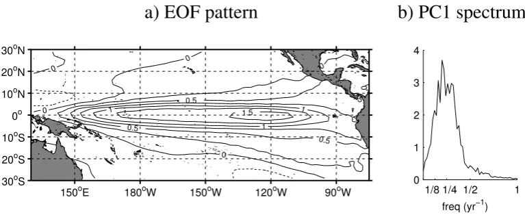
In Fig. 1a we present the first empirical orthogonal func-tion (EOF) of the SST anomalies in the equatorial Pacific from the ESSENCE ensemble. The first mode contains 72 % of the variability, and its principal component has a broad spectral peak ranging between 2.5 and 8 yr periods (Fig. 1b). This is in good agreement with the typical 3 and 6 yr period obtained for the first EOF in the HadiSST data set (van Old-enborgh et al., 2005). The amplitude of the first EOF is how-ever too strong, and the westerly extension of cold tongue is too large (see also van Oldenborgh et al. (2005); Jungclaus et al. (2006)). These issues also appear in the NINO3 and NINO4 indices, as their standard deviations are, respectively, 0.6 and 0.8◦C higher than those retrieved from the Reynolds optimal interpolation (see Table 1). The NINO3 and NINO4 indices are constructed by calculating the average SST anomaly in the region [150◦W–90◦W]×[5◦S–5◦N] and [160◦E–150◦W]×[5◦S–5◦N], respectively (Trenberth and Hoar, 1997).

It is well known that the eastern Pacific NINO3 index is skewed to warm values and the western Pacific NINO4 index is skewed to cold values (Trenberth and Hoar, 1997; Burg-ers and Stephenson, 1999). Capturing the rights statistics is not easily assured in climate models, as was shown by van Oldenborgh et al. (2005). Although the ECHAM5/MPI-OM model gives a correct sign of the skewness for NINO3 and NINO4, the statistics do not strongly deviate from a Gaus-sian distribution. The cold La Ni˜na events are as strong and frequent as the warm El Ni˜no events (Roeckner et al., 2003). This is most prominent in the NINO3 index, for which the skewness is too small (Table 1).

(3)

W. Kramer and H. A. Dijkstra: Optimal observations for ENSO prediction 223

Figures

a) EOF pattern

b) PC1 spectrum

0 0

0

0.5 0.5

1 1

1 1.5

150oE 180oW 150oW 120oW 90oW

30oS 20oS 10oS 0o 10oN 20oN 30oN

1/8 1/4 1/2 1

0 1 2 3 4

freq (yr−1)

Fig. 1.

a) The first EOF of the SST anomalies in the equatorial Pacific. b) Power spectrum

of the first principle component (PC1), which is normalized to have unit variance.

a) Reynolds b) ESSENCE

kurt(SST)

0 10 20 30 40 50 60

skew(SST)

−4 −2 0 2 4 6

skew(SST)

−4 −2 0 2 4 6

60˚N–75˚N 60˚S–75˚S 45˚N–60˚N 45˚S–60˚S

30˚N–45˚N 30˚S–45˚S 15˚N–30˚N 15˚S–30˚S

0˚N–15˚N 0˚S–15˚S

weak multip. noise

Fig. 2.

Skewness kurtosis scatter plot for SST from the Reynolds analysis and the

ESSENCE data set. The data points relate to fixed locations, which are collected in

lati-tudinal bands. Points can not be situated in the grey area as the general statistical bound

requires that kurtosis

≥

skewness

2

−

2. The drawn curve relates to the lower parabolic

bound kurtosis

≥

3/2 skewness

2

(Sura and Sardeshmukh, 2008).

Fig. 1. (a) The first EOF of the SST anomalies in the equatorial Pacific. (b) Power spectrum of the first principle component (PC1), which is normalized to have unit variance.

Table 1. Statistical moments of the NINO3 and NINO4 indices from the ESSENCE ensemble simulation and the HadiSST (Rayner et al., 2003) and Reynolds and Smith (1994) SST data analysis; N is the number of data points.

NINO3 NINO4

ESSENCE HadiSST Reynolds ESSENCE HadiSST Reynolds

variance 1.5435 0.6196 0.9682 1.2983 0.3177 0.5162

skewness 0.0235 0.7417 0.9412 −0.1581 −0.1408 −0.5655 kurtosis −0.1374 1.1542 1.5794 −0.3873 −0.3524 −0.5658

N 12 440 1680 348 12 440 1680 348

One of the drawbacks of looking at the statistical moments of the NINO indices is that the deviations can be caused by the shift of the ENSO pattern. For this purpose we per-formed a pointwise calculation of the skewness and kurtosis in the SSTA. A scatter plot of these quantities is presented in Fig. 2. A general statistical lower bound for the sis can be formulated in terms of the skewness, i.e. kurto-sis≥skewness2−2. Sura and Sardeshmukh (2008) derived a more strict lower bound: kurtosis≥3/2 skewness2under the assumption that the gustiness of the sea surface winds leads to a weak multiplicative-noise forcing of the sea-surface tem-perature anomalies. Sura and Sardeshmukh (2008) found that daily global SSTA data from the Reynolds optimal interpo-lation showed a surprising conformity to the stricter lower bound (see also Fig. 2). In this benchmark the ESSENCE model compares more favourably to the observational data than for the statistical moments of the NINO indices. Overall, the spread in the scatter plot is surprisingly similar. A closer inspection reveals that the ESSENCE data points in the equa-torial band (15◦S–15◦N) are more negatively skewed than those calculated from the Reynolds data set.

2.2 The cold tongue and warm pool El Ni ˜no events

As the ECHAM5/MPI-OM is one of the better models for ENSO variability, it is interesting whether it also contains

both the classical cold tongue (CT) El Niño and the warm pool (WP) El Niño events. For classifying all El Niño events in the ESSENCE ensemble, we use a method similar to the one used by Kug et al. (2010) on data from a 500 yr prein-dustrial (1860 levels) simulation with the GFDL 2.1 coupled GCM. As this model also produces a too westerly El Niño SST pattern, they shifted the regions for determining the NINO3 and NINO4 indices 20◦ westward. All years with at least one of the modified indices, NINO3m or NINO4m, exceeding 0.5◦_{C in ND(0)J(1) (November, December and}

January in the next year) are classified as El Ni˜no events. They find that, out of these 205 events, the 121 events with NINO3m>NINO4m are considered to be the canonical cold tongue events and 84 with NINO4m>NINO3m are counted as warm pool events.

Applying the same criteria to the ESSENCE data yields 306 cold tongue and 55 warm pool El Niño events in 1000 yr (20 runs of 50 yr). Under these conditions we find WP El Niño events are less frequent than in Kug et al. (2010). If we add the additional constraint that in the previ-ous year (YEAR(-1)) there were no El Niño conditions, then we retrieve 194 CT events and only 15 WP events. This in-dicates that, in the ESSENCE ensemble, WP-like conditions are more likely in the year following El Niño conditions than after neutral or La Niña conditions.

(4)

224 W. Kramer and H. A. Dijkstra: Optimal observations for ENSO prediction

Figures

a) EOF pattern

b) PC1 spectrum

0 0

0

0.5 0.5

0.5

1 1

1 1.5

150oE 180oW 150oW 120oW 90oW

30oS 20oS 10oS 0o 10oN 20oN 30oN

1/8 1/4 1/2 1 0

1 2 3 4

freq (yr−1)

Fig. 1.

a) The first EOF of the SST anomalies in the equatorial Pacific. b) Power spectrum

of the first principle component (PC1), which is normalized to have unit variance.

a) Reynolds b) ESSENCE

kurt(SST)

0 10 20 30 40 50 60

skew(SST)

−4 −2 0 2 4 6

skew(SST)

−4 −2 0 2 4 6

60˚N–75˚N 60˚S–75˚S 45˚N–60˚N 45˚S–60˚S

30˚N–45˚N 30˚S–45˚S 15˚N–30˚N 15˚S–30˚S

0˚N–15˚N 0˚S–15˚S

weak multip. noise

Fig. 2.

Skewness kurtosis scatter plot for SST from the Reynolds analysis and the

ESSENCE data set. The data points relate to fixed locations, which are collected in

lati-tudinal bands. Points can not be situated in the grey area as the general statistical bound

requires that kurtosis

≥

skewness

2

−

2

. The drawn curve relates to the lower parabolic

bound kurtosis

≥

3/2 skewness

2

(Sura and Sardeshmukh, 2008).

21

Fig. 2. Skewness kurtosis scatter plot for SST from the Reynolds analysis and the ESSENCE data set. The data points relate to fixed locations, which are collected in latitudinal bands. Points cannot be situated in the grey area as the general statistical bound requires that kurtosis≥skewness2−2. The drawn curve relates to the lower parabolic bound kurtosis≥3/2 skewness2(Sura and Sardeshmukh, 2008).

The Hovm¨oller diagram of the composite SST anomalies on the Equator for the isolated CT (194) and the WP (15) events, presented in Fig. 3, compares well to Fig. 7 in Kug et al. (2010). For both type of events, there is a warming in the eastern Pacific in late boreal spring/early boreal summer. For the cold tongue events, the region with elevated SST lev-els persists during the year and extends to the western Pa-cific; the location of maximum SST remains in the east. Dur-ing warm pool events there is a coolDur-ing of the eastern Pacific after the warming in boreal spring. In boreal winter a strong warming occurs west of the dateline. Including the prolonged 2 yr (YEAR(-1) and YEAR(0)) El Ni˜no events gives elevated SSTs ranging from boreal winter to summer for WP events over the whole equatorial Pacific in YEAR(0), but does not significantly change the picture of a warming centred in the western Pacific in boreal winter.

3 Methodology

We intend to use the control ESSENCE ensemble to de-termine how observations improve the predictability of the ENSO events. Assimilating real observations would lead to a poor analysis as there is no one-to-one mapping between ob-servations and model data. For this reason we opt to perform an identical twin experiment, where one model realization is used as a synthetic truth. Observations are then produced by adding a normal-distributed observation error to specific model variables.

The ESSENCE data set provides a Monte Carlo sample of the climatological probability distributionq(x). Working with the probability density function (pdf) of the full state vector x of the climate model is bothersome and unneces-sary. We are only interested in predicting El Ni˜no; as such we want the univariate probability distribution q(s) where s is one of the NINO indices. The 20 ensemble members, each 50 yr long, are cut into one-year segments yielding a total number ofN=1000 segments. These segments are as-sumed to be independent although there certainly is a corre-lation between one year and the next year. The samples are also not identically distributed as some belong to the same ensemble member, and others belong to different ensemble members. The choice to be made is between a larger sam-ple size or a better samsam-ple independence. We have repeated the experiments with leaving the odd years out, and this does not significantly change the results. These segments not only sample the equilibrium probability distribution, but also con-tain the time evolution. The El Ni˜no variability typically has a period of 3–5 yr. The absence of longer time scales in the SST variability yields a better sampling density. Taking seg-ments shorter than one year is not viable as ENSO dynamics are strongly season dependent. Without any up-to-date data or observations, the equilibrium distribution is the best pre-diction/description for the current state of the equatorial Pa-cific.

The assimilation method described in the following para-graphs was also used to determine the impact of observations

(5)

W. Kramer and H. A. Dijkstra: Optimal observations for ENSO prediction 225

a) cold tongue

b) warm pool

−0.5

0

0 0.5

0.5

1

1.5

2

120_°E 180_° 120_°W Jan

Apr Jul Oct Jan Apr Jul Oct

YEAR(0)

YEAR(1)

−0.5

0

0 ₀

0

0.5

1

1 1.5

120_°E 180_° 120_°W Jan

Apr Jul Oct Jan Apr Jul Oct

Fig. 3.

Hovm¨ollerplot of the composite SST anomalies on the equator for a) years satisfying

the cold tongue conditions, and b) years satisfying the warm pool conditions. The contour

spacing is

0

.

25

◦

C and temperatures over

0

.

5

◦

C are coloured grey.

a) sea surface temperature

b) zonal wind speed

c) thermocline depth

Fig. 4.

Composite over 20 CT El Ni˜no events of the predictive power, PP(NINO3), gained

by assimilating observations in JFM(0) for a given location (left panels); and the composite

predictive power remaining in June (right panels). Assimilated quantities are a) the SST, b)

the zonal wind speed or c) the thermocline depth.

Fig. 3. Hovm¨oller plot of the composite SST anomalies on the Equator for (a) years satisfying the cold tongue conditions, and (b) years satisfying the warm pool conditions. The contour spacing is .25◦C, and temperatures over 0.5◦C are coloured grey.

on the predictability of the Kuroshio Extension (Kramer et al., 2012). The purpose of assimilating observations is to decrease the spread in the ensemble. A measure (Schneider and Griffies, 1999) for the gained skill of the analysis pdf, in-dicated below byp(s), is the predictive power (PP) defined by

PP=1−σ

2 p

σ_q2, (1)

whereσ_p2 andσ_q2 are the analysis variance and the clima-tology variance of s, respectively. The predictive power is zero for an ensemble which does not provide additional in-formation over the climatology distribution. When the anal-ysis improves, the PP goes asymptotically towards one, the value related to a fully deterministic state. As discussed by Schneider and Griffies (1999), Eq. (1) is a simplification of the more general entropy-based formulation for the predic-tive power. Equation (1) results from assuming a Gaussian distribution for bothp(s)andq(s). In the previous section we found that the NINO3 index is only weakly non-Gaussian in the ESSENCE data set. As such we can use the definition in Eq. (1) for predictive power based on the variance of the analysis.

The basic idea is that an observation changes, the weight wi of a one-year segment, which is defined by its state vec-torxi(t ). We then obtain a better estimation of the current

state from the weighted ensemble, from which we can cal-culate statistics like the mean and variance. Sequential im-portance sampling (SIS) is used for changing the weights with the information from a number of discrete observa-tions. When an observationyk becomes available att=tk

the weight change (at each point in the domain) follows from

Bayes’ theorem, yielding

wi_k=p(yk|x

i k)

p(yk)

w_ki₋₁ fori=1. . . N. (2)

Here,p(yk|x_ki)is the probability density function of the

ob-servations given the model statex_ki, and p(yk)is the

prob-ability density function of the observation. The latter can be considered as a normalization factor, which assures that the total weight is equal to one. From the measurement er-ror statistics, the shape of the function p(yk|x) is known,

where x now refers to the true state. When using a prior ensemble, we change the true state with the model state x_ki from the ensemble. Assuming that the error tion of the measurement is a multivariate normal distribu-tion,f (yk)∼exp[−(yk−yk)T6−1(yk−yk)]with6the

er-ror covariance matrix, and, for a Gaussian distributed prior, p(yk|x_ki)is given by

p(yk|xki)∼exp[−

1

2(yk−H (x

i

k))T(6+B)−1(yk−H (xik))],

(3) whereH (xi_k)is the mean of the prior andBits covariance. In our set-up the observed quantities are explicitly available in the model, and the observation operatorHis simply selecting the model equivalents from the full state vector.

Choosing the magnitude of the error covariance is partly determined by the number of ensemble members that are available. An accurate measurement effectively discards a large number of particles, and only particles that are close to observation remain. A strongly degenerated ensemble, how-ever, does not yield an accurate estimate forσp. When one

(6)

226 W. Kramer and H. A. Dijkstra: Optimal observations for ENSO prediction

a) cold tongue

b) warm pool

−0.5

0

0 0.5

0.5

1

1 1.5

1.5

2

120°E 180° 120°W

Jan Apr Jul Oct Jan Apr Jul Oct

YEAR(0)

YEAR(1)

−0.5 0

0

0 ₀

0

0 0.5

0.5

1

1 1.5

120°E 180° 120°W

Jan Apr Jul Oct Jan Apr Jul Oct

Fig. 3.

Hovm¨ollerplot of the composite SST anomalies on the equator for a) years satisfying

the cold tongue conditions, and b) years satisfying the warm pool conditions. The contour

spacing is

0

.

25

◦

C and temperatures over

0

.

5

◦

C are coloured grey.

a) sea surface temperature

b) zonal wind speed

Fig. 4.

by assimilating observations in JFM(0) for a given location (left panels); and the composite

predictive power remaining in June (right panels). Assimilated quantities are a) the SST, b)

the zonal wind speed or c) the thermocline depth.

22

Fig. 4. Composite over 20:00 CT El Ni˜no events of the predictive power, PP(NINO3), gained by assimilating observations in JFM(0) for a given location (left panels); and the composite predictive power remaining in June (right panels). Assimilated quantities are (a) the SST, (b) the zonal wind speed and (c) the thermocline depth.

particle has all the weight,σp vanishes and the predictive

power goes to unity. When observing one quantity, say the SST, we set the observational error to 0.2σSST(x)of the

cli-matology. This guarantees that in regions with low variabil-ity we can still detect whether there is a useful signal, as the signal-to-noise ratio is constant. When two kinds of observa-tions are assimilated simultaneously, say SST and zonal wind speed, the error is set to 0.2

√

2σSST(x)and 0.2

√

2σwind(x).

As the focus of this study is on the impact of observation lo-cation on ENSO predictability, and not on simulating a real operational observation system, this is a legitimate choice.

In the following section we assimilate monthly averaged data over three months. These three observations are gener-ated by adding a random observational error to the synthetic truth. We are not interested in these specific three realiza-tions of the synthetic observarealiza-tions, but would like to incor-porate the error statistics. This is done by using a bootstrap-ping algorithm to determinep(s)andσp(s), where the data

assimilation is repeated for 100 realizations of the stochastic observations.

4 The impact of observations for monitoring ENSO

4.1 Optimal observation locations for sea surface tem-perature, zonal wind speed and thermocline depth

The first question we want to answer is where to optimally measure SST, zonal wind speed and thermocline depth to de-termine the state of the ENSO as measured by the NINO in-dices and its future development. There are two important metrics involved for determining efficient observations. The first is the predictive power, indicated by PP0, of the

ensem-ble after the observation period of three months. The second is the predictive power, indicated by PP3 m, after the

ensem-ble has been aensem-ble to develop freely for another three months. So, we if measure in JFM(0), PP0relates to March and PP3 m

to June.

PP0 is a measure of how efficient the observations are in

decreasing the variance of the ensemble. This quantity av-eraged over 20 synthetic truths is shown in the left panels of Fig. 4. All synthetic truths are years when a CT El Ni˜no event occurs. The plot shows the PP related to the location

(7)

W. Kramer and H. A. Dijkstra: Optimal observations for ENSO prediction 227

a) sea surface temperature

b) zonal wind speed

Fig. 5.

by assimilating observations in MAM(0) for a given location (left panels); and the

compos-ite predictive power remaining in August (right panels). Assimilated quantities are a) the

SST, b) the zonal wind speed or c) the thermocline depth.

Fig. 5. Composite over 20:00 CT El Ni˜no events of the predictive power, PP(NINO4), gained by assimilating observations in MAM(0) for a given location (left panels); and the composite predictive power remaining in August (right panels). Assimilated quantities are (a) the SST, (b) the zonal wind speed and (c) the thermocline depth.

of the assimilated observations. In regions with a high pre-dictive power, there is significant signal which is correlated to the NINO3 index. If for a given location there is no cor-related signal component or this component is exceeded by the observation error, the predictive power remains low. The pattern with large predictive power increase conforms with the ENSO pattern (Fig. 1) with the largest values of PP0

lo-calized inside the NINO3 box. Observations of zonal wind speed are less efficient in reducing the ensemble spread; the main correlated region is here east of New Guinea along the Equator. Observing the thermocline depth between 120◦W and 90◦W is more efficient for retrieving the NINO3 index. The depth of the 15◦C isotherm is used as a proxy for the thermocline depth.

After the assimilation stage, the weighted ensemble evolves freely (providing a probabilistic forecast), and over time the ensemble spread increases due the chaotic ENSO dynamics. Essentially, this phase is a predictability study of the first kind. The uncertainty in the initial conditions, i.e. the state at the end of the assimilation stage, is reduced with

information from one specific location. If we focus on the spring predictability barrier, the important metric is the pre-dictive power that remains in June. This prepre-dictive power PP3 mis plotted in the right panels of Fig. 4. For this case the

predictability barrier is clearly visible, as the PP of the en-semble strongly reduces over the total Pacific. Observations of SST and thermocline depth in the region around 120◦W seem to provide the most useful information for predicting the NINO3 index. If the second, freely evolving stage is out-side the April/May period, PP3 mremains high (not shown).

The pattern of high PP values does not significantly change when the experiment is initiated in other months.

The NINO4 index is strongly correlated with NINO3 in-dex with a lag of two months. This correlation is related to the westward propagation of SST anomalies by equatorial Kelvin waves. This becomes clear if we look at the ensem-ble analysis for NINO4, as is illustrated by PP(NINO4) in Fig. 5. Here, the observations in MAM(0) are assimilated, and the predictive power is analysed in March and August. SST observations at the Equator between 150◦E and 120◦W

(8)

a) zonal wind speed

b) thermocline depth

c) zonal wind speed

d) thermocline depth

Fig. 6.

Composite over 20 CT El Ni˜no events of the predictive power, PP of NINO3

remain-ing in June after assimilatremain-ing SST from

110

°W in JFM(0) and (at a given location) either

a) zonal wind speed or b) the thermocline depth. The same for the lower panels but now

for the PP of NINO4 remaining in August after assimilating SST at

140

°W in MAM(0) and

either c) zonal wind speed or d) the thermocline depth.

Fig. 6. Composite over 20:00 CT El Ni˜no events of the predictive power, PP of NINO3 remaining in June after assimilating SST from 110◦W in JFM(0) and (at a given location) either (a) zonal wind speed and (b) the thermocline depth. The same for the lower panels but now for the PP of NINO4 remaining in August after assimilating SST at 140◦W in MAM(0) and either (c) zonal wind speed and (d) the thermocline depth.

are best for monitoring the NINO4 index. Note that the PP pattern in Fig. 5 also corresponds to the ENSO pattern, but high PP is also located in the western part. SST data from the region from 150◦W to 120◦W contain better information for predicting the NINO4 index three months in advance. Useful locations for measuring zonal wind speeds are more concen-trated in the western Pacific, directly bordering New Guinea island. The areas where the thermocline depth provides use-ful information for the NINO4 index are in the western Pa-cific (related to pattern of the wind bursts) and in the eastern part of the Pacific. The latter area relates to the optimal pat-tern for the NINO3 index (Fig. 4c), and hence this is just another manifestation of the correlation between the NINO3 and NINO4 regions.

The predictive power for the NINO4 index does not drop as much in boreal spring as for the NINO3 index. This in-dicates that the instability, which is the cause of the spring predictability barrier, starts in the eastern Pacific. The better predictability for NINO4 lasts till July, when the strongest drop of PP3 m occurs. The predictability barrier we find in

the April/May period in principle can be either related to the spring barrier or the growth-phase barrier. In the results pre-sented here, the synthetic truth always relates to a year with a CT El Ni˜no event. However, if we select only La Ni˜na years or only neutral years, results do not change. Hence, there is an apparent predictability barrier in spring for all years, and no indications appear for a growth-phase barrier.

4.2 Combining SST observations with thermocline or zonal wind speed data

The SST observations are best for monitoring the NINO in-dices. They essentially already fix the phase of the ENSO during the three-month observation period. The optimal lo-cation for reconstructing the NINO3 index is on the Equator at 110◦W, while for NINO4 it is at 140◦W. Predictability can be improved by assimilating additional data. In Fig. 6 we combine SST data from (110◦W, 0◦N) with observations of the thermocline depth or zonal wind speed. The green back-ground gives the PP3 mresulting from the SST observations.

Measuring the thermocline depth between 180 and 120◦W gives a significant increase of PP3mover the one obtained by

assimilating only SST. It is most likely that these additional observations capture the eastward travelling Kelvin wave. No increase of PP3 mis found in the region (110◦W–90◦W)

with a strong correlation between the thermocline depth and NINO3 index (see Fig. 4c). Information from this region is already provided by the SST observations. Assimilation of zonal wind speed observations in addition to the SST data does not seem to improve predictability of the NINO3 index. In the previous section we already observed the NINO4 in-dex is better predictable than NINO3. The background value of PP3 m in Fig. 6c and d resulting from the SST

observa-tions is higher than those in Fig. 6a and b. Again we gain a significant increase of PP by observing the thermocline depth in addition to SST.

(9)

W. Kramer and H. A. Dijkstra: Optimal observations for ENSO prediction 229

5 Conclusions

The 20-member control ensemble from the ESSENCE project with a fixed CO2 level provides us a large Monte

Carlo sample of the ENSO climatology. The data contain reasonably realistic ENSO variability on a 2.5 to 8 yr time scale. Important shortcomings of the ECHAM5/MPI-OM are the overly large SST variability and the too westerly extent of the ENSO pattern. A pointwise view of the SST skew-ness and kurtosis provides a good comparison to values ob-tained from the Reynolds optimal interpolation (Reynolds and Smith, 1994). Moreover, this result confirms the pic-ture that random wind gustiness leads to weak multiplicative-noise forcing of the sea-surface temperature anomalies (Sura and Sardeshmukh, 2008). The skewness in the equatorial re-gions seems to be more negatively skewed for the ESSENCE data. For the NINO indices, the statistics are too Gaussian with relatively small skewness and kurtosis values compared to observations.

Localized monthly averaged observations of SST, zonal wind speed and thermocline depth were assimilated using sequential importance sampling. The effective skill of these observations in reducing the ensemble spread is measured by the predictive power (Schneider and Griffies, 1999). This allows us to determine optimal locations for monitoring the NINO indices. After the assimilation of the observations, we investigated how the weighted ensemble performs as a nine-month probabilistic forecast of the ENSO. The predictive power remaining after three months reveals optimal obser-vation locations for enhancing predictability.

The data from the ESSENCE ensemble clearly exhibit the spring predictability barrier as a large drop in predictive power is observed during April/May. This drop is indepen-dent of the phase of the ENSO. As such we do not observe the growth-phase predictability barrier. The predictability barrier first becomes apparent for the NINO3 index. During this time the NINO4 index is much better predictable. The largest drop in PP for NINO4 occurs in July.

We focus on the spring predictability barrier when search-ing for optimal locations for predictsearch-ing the ENSO through two NINO3 indices. Efficient SST observations for moni-toring are localized in the ENSO pattern: in the eastern Pa-cific for the NINO3 index and in the western PaPa-cific for the NINO4 index. For a three-month forecast, however, a more easterly location (140◦W) yields better predictive power for the NINO4 index. It is well known that the NINO4 index is lagging the NINO3 index by two months. SST observa-tions at a single location already give much information on the phase of the ENSO as SST is spatially correlated with the ENSO pattern.

Observations of the thermocline depth in addition to SST observations yield an increase in predictive power over the predictability barrier. An improved forecast of NINO3 up to June results from thermocline observations in the JFM time frame at 150◦W, which seem to capture a Kelvin wave.

Zonal wind speed observations, mainly localized in western Pacific, provide information for reconstructing the NINO3 and NINO4 indices. They, however, do not yield additional information to the SST observations.

Predictability studies often aim to find the perturba-tion (pattern) of the initial state which exhibits the fastest growth (Moore and Kleeman, 1996; Chen et al., 1997; Duan et al., 2009). A possible observation strategy is then to choose observation locations which minimize the amplitude of the optimal perturbation in the initial conditions. The approach we take is in essence the reverse; we determine the optimal locations, which minimizes the uncertainty of the forecast after a certain lead time. One of the advantages is that we can assimilate observations during a specific period and in-corporate observation error statistics. Major drawback of the method is the number of ensemble members required. As-similating accurate observations focuses most of the weight on a few particles. Hence, the number of ensemble members determines the number of observations (sequential and/or si-multaneous) that can be made with a predetermined observa-tional error before the ensemble degenerates.

As we assimilate observations over a three-month period, quantities that lead or lag the NINO indices by two months can contribute useful information. Essentially, the integrated effect of the observations is used by the data assimilation. The patterns of observation locations which yield high pre-dictive power can also be related to the optimal perturba-tion patterns for initial condiperturba-tions. For the spring predictabil-ity barrier, Chen et al. (1997) find a perturbation pattern, which maximizes SST variability, with the largest amplitude in eastern Pacific at 110◦_{W and 5}◦_{S. Moore and Kleeman}

(1996) locate the optimal perturbation for maximizing total atmospheric and oceanic perturbation energy around 160◦_W.

Duan et al. (2009) obtain initial errors with the extrema lo-cated at 150◦W and 110◦W that significantly contribute to the spring predictability barrier. All these locations are in the eastern Pacific, which is in agreement with the retrieved optimal locations for increasing the predictive power after a three-month forecast.

Acknowledgements. The ESSENCE project, lead by Wilco Hazeleger (KNMI) and Henk Dijkstra (UU), was carried out with support of DEISA and NCF (through NCF projects NRG-2006.06, CAVE-06-023 and SG-06-267). We thank the DEISA Consortium (co-funded by the EU, FP6 projects 508830/031513) for support within the DEISA Extreme Computing Initiative. The authors thank Andreas Sterl (KNMI), Camiel Severijns (KNMI), and HLRS and SARA staff for technical support.

Edited by: W. Hsieh

Reviewed by: P. J. van Leeuwen and one anonymous referee

(10)

References

Battisti, D. S. and Hirst, A. C.: Interannual variability in a tropi-cal atmosphere-ocean model: Influence of the basic state, ocean geometry and nonlinearity, J. Atmos. Sci., 46, 1687–1712, 1989. Burgers, G. and Stephenson, D. B.: The “Normality” of El Ni˜no,

Geophys. Res. Lett., 26, 1027–1030, 1999.

Chen, Y. Q., Battisti, D. S., Palmer, T. N., Barsugli, J., and Sarachik, E. S.: Study of the predictability of tropical SST in a coupled atmosphere-ocean model using singular vector analysis: The role of the annual cycle and the ENSO cycle, Mon. Wea. Rev., 125, 831–845, 1997.

Duan, W., Liu, X., Zhu, K., and Mu, M.: Exploring the initial error that causes a significant predictability barrier for El Ni˜no events, J. Geophys. Res., 114, C04022, 1–12, 2009.

Federov, A. V.: The response of the coupled ocean-atmosphere to westerly wind bursts, Q. J. Roy. Meteorol. Soc., 128, 1–23, 2002. Federov, A. V., Harper, S., Philander, S., Winter, B., and Wittenberg, A.: How predictable is El Ni˜no?, Bull. Amer. Meteor. Soc., 911– 919, 2003.

Jungclaus, J. H., Keenlyside, N., Haak, H., Luo, J.-J., Latif, M., Marotzke, J., Mikolajewicz, U., and Roeckner, E.: Ocean circulation and tropical variability in the coupled model ECHAM5/MPI-OM, J. Climate, 19, 3952–3972, 2006.

Kramer, W., Dijkstra, H. A., Pierini, S., and van Leeuwen, P. J.: Measuring the impact of observations on the predictability of the Kuroshio Extension in a shallow-water model, J. Phys. Oceanogr., 42, 3–17, 2012.

Kug, J.-S., Choi, J., An, S.-I., Jin, F.-F., and Wittenberg, A. T.: Warm Pool and Cold Tongue El Ni˜no Events as Simulated by the GFDL 2.1 Coupled GCM, J. Climate, 23, 1226–1239, 2010.

Latif, M., Barnett, T. P., Cane, M. A., Fl¨ugel, M., Graham, N. E., von Storch, H., Xu, J.-S., and Zebiak, S. E.: A review of ENSO prediction studies, Clim. Dynam., 9, 167–179, 1994.

McPhaden, M. J., Busalacchi, A. J., Cheney, R., Donguy, J. R., Gage, K. S., Halpern, D., Ji, M., Julian, P., Meyers, G., Mitchum, G. T., Niiler, P. P., Picaut, J., Reynolds, R. W., Smith, N., and Takeuchi, K.: The tropical ocean-global atmosphere observing system: a decade of progress, J. Geophys. Res, 103, 14169– 14240, 1998.

Moore, A. M. and Kleeman, R.: The dynamics of error growth and predictability in a coupled model of ENSO, Q. J. Roy. Meteorol. Soc., 122, 1405–1446, 1996.

Mu, M., Duan, W., and Wang, B.: Season-dependent dynamics of nonlinear optimal error growth and ENSO predictability in a the-oretical model, J. Geophys. Res., 112, D10113, 1–10, 2007. Neelin, J. D.: The slow sea surface temperature mode and the

fast-wave limit: analytic theory for tropical interannual oscillations and expactations in a hybrid coupled model, J. Atmos. Sci., 48, 584–606, 1991.

Rayner, N. A., Parker, D. E., Horton, E. B., Folland, C. K., Alexan-der, L. V., Rowell, D. P., Kent, E. C., and Kaplan, A.: Global analyses of sea surface temperature, sea ice, and night marine air temperature since the late nineteenth century, J. Geophys. Res., 108, 4407, 1–22, 2003.

Reynolds, R. W. and Smith, T. M.: Improved global sea surface temperature analyses using optimum interpolation, J. Climate, 7, 929–948, 1994.

Roeckner, E., B¨auml, G., Bonaventura, L., Brokopf, R., Esch, M., Giorgetta, M., Hagemann, S., Kirchner, I., Kornblueh, L., Manzini, E., Rhodin, A., Schlese, U., Schulzweida, U., and Tompkins, A.: The atmospheric general circulation model ECHAM 5. Part 1: Model description, Tech. Rep. 349, Max-Planck-Institute for Meteorology, 2003.

Roeckner, E., Brokopf, R., Esch, M., Giorgetta, M., Hagemann, S., Kornblueh, L., Manzini, E., Schlese, U., and Schulzweida, U.: Sensitivity of simulated climate to horizontal and vertical reso-lution in the ECHAM5 atmosphere model, J. Climate, 19, 3771– 3791, 2006.

Samelson, R. M. and Tziperman, E.: Instability of the chaotic ENSO: The growth-phase predictability barrier, J. Atmos. Sci., 58, 3613–3625, 2001.

Schneider, T. and Griffies, S. M.: A conceptual framework for pre-dictability studies, J. Climate, 12, 3133–3155, 1999.

Sterl, A., Severijns, C., Dijkstra, H. A., Hazeleger, W., van Olden-burgh, G. J., van den Broeke, M., van den Hurk, B., van Leeuwen, P. J., and van Velthoven, P.: When can we expect extremely high surface temperatures?, Geophys. Res. Lett., 35, L14703, 1–5, 2008.

Sura, P. and Sardeshmukh, P. D.: A Global View of Non-Gaussian SST Variability, J. Phys. Oceanogr., 38, 639–647, 2008. Trenberth, K. E. and Hoar, T. J.: El Ni˜no and climate change,

Geo-phys. Res. Lett., 24, 3057–3060, 1997.

van Oldenborgh, G. J., Philip, S. Y., and Collins, M.: El Ni˜no in a changing climate: a multi-model study, Ocean Sci., 1, 81–95, doi:10.5194/os-1-81-2005, 2005.

Webster, P. J.: The annual cycle and the predictibability of the trop-ical coupled ocean-atmosphere system, Meteorol. Atmos. Phys., 56, 33–55, 1995.

Webster, P. J. and Yang, S.: Monsoon and ENSO: Selectively inter-active systems, Q. J. Roy. Meteorol. Soc., 118, 877–926, 1992. Yu, Y., Mu, M., and Duan, W.: Does model parameter error cause a

significant spring predictability barrier for El Ni˜no events in the Zebiak-Cane model, J. Climate, 25, 1263–1277, 2012.

Zebiak, S. E. and Cane, M. A.: A model El-Ni˜no southern oscilla-tion, Mon. Wea. Rev., 115, 2262–2278, 1987.