www.earth-surf-dynam.net/4/757/2016/ doi:10.5194/esurf-4-757-2016
© Author(s) 2016. CC Attribution 3.0 License.
The sensitivity of landscape evolution models to spatial
and temporal rainfall resolution
Tom J. Coulthard and Christopher J. Skinner
Department of Geography, Environment and Earth Sciences, University of Hull, Hull, UK
Correspondence to:Tom J. Coulthard ([email protected])
Received: 11 January 2016 – Published in Earth Surf. Dynam. Discuss.: 20 January 2016 Revised: 26 July 2016 – Accepted: 28 August 2016 – Published: 30 September 2016
Abstract. Climate is one of the main drivers for landscape evolution models (LEMs), yet its representation is
often basic with values averaged over long time periods and frequently lumped to the same value for the whole basin. Clearly, this hides the heterogeneity of precipitation – but what impact does this averaging have on erosion and deposition, topography, and the final shape of LEM landscapes? This paper presents results from the first systematic investigation into how the spatial and temporal resolution of precipitation affects LEM simulations of sediment yields and patterns of erosion and deposition. This is carried out by assessing the sensitivity of the CAESAR-Lisflood LEM to different spatial and temporal precipitation resolutions – as well as how this interacts with different-size drainage basins over short and long timescales. A range of simulations were carried
out, varying rainfall from 0.25 h×5 km to 24 h×Lump resolution over three different-sized basins for 30-year
durations. Results showed that there was a sensitivity to temporal and spatial resolution, with the finest leading to > 100 % increases in basin sediment yields. To look at how these interactions manifested over longer timescales, several simulations were carried out to model a 1000-year period. These showed a systematic bias towards greater erosion in uplands and deposition in valley floors with the finest spatial- and temporal-resolution data. Further tests showed that this effect was due solely to the data resolution, not orographic factors. Additional research indicated that these differences in sediment yield could be accounted for by adding a compensation factor to the model sediment transport law. However, this resulted in notable differences in the topographies generated, especially in third-order and higher streams. The implications of these findings are that uncalibrated past and present LEMs using lumped and time-averaged climate inputs may be under-predicting basin sediment yields as well as introducing spatial biases through under-predicting erosion in first-order streams but over-predicting erosion in second- and third-order streams and valley floor areas. Calibrated LEMs may give correct sediment yields, but patterns of erosion and deposition will be different and the calibration may not be correct for changing climates. This may have significant impacts on the modelled basin profile and shape from long-timescale simulations.
1 Introduction
Landscape evolution models (LEMs) have been extensively developed to understand how Earth surface processes influ-ence drainage basin dynamics and morphology. One of the important forcings of erosion and morphodynamic change in these models is climate – usually in the form of precip-itation. However, all LEMs use some degree of spatial and temporal averaging for their driving climate or precipitation data. Spatially, rainfall (or climate parameters) are usually
are important practical reasons for using averaged or coarse spatial- and temporal-resolution precipitation data, including data availability, model parsimony and model efficiency. Us-ing spatially lumped climate values makes models simpler to construct and coarse temporal resolutions can make them faster to run by enabling longer time steps. Furthermore, the availability of high temporal- and spatial-resolution precip-itation data is often poor – especially if the quality and va-lidity of the data are considered. Finally, many LEM studies run over tens to thousands of years where it is impossible to generate or reconstruct suitable records of precipitation of a high resolution.
There has been a limited exploration of precipitation resolution impacts in previous LEM studies; Sólyom and Tucker (2007) argued that over the long timescales that LEMs are often applied, spatial effects will become less im-portant. For example, as the modelled period of a simula-tion increases, the probability for separate convective rain-fall cells hitting all parts of the basin increases. Additionally, Sólyom and Tucker (2007) suggest that temporal effects be-come less important when the basin is of sufficient size that hydrological travel times from the top to the bottom of the basin are greater than the duration of precipitation events.
As morphodynamic changes within basins are heavily as-sociated with basin hydrology, further insights may be drawn from hydrological modelling studies – where the influence of the spatial and temporal resolution of rainfall inputs has been discussed for over 3 decades (Lobligeois et al., 2014). In this literature, there is a general agreement that finer detail in the representation of spatial and temporal variability of rainfall in a hydrological model will improve the outputs, especially when observing hydrographs from a single event (Beven and Hornberger, 1982; Bronstert and Bárdossy, 2003; Finnerty et al., 1997; Hearman and Hinz, 2007; Ogden and Julien, 1994; Wainwright and Parsons, 2002; Wilson et al., 1979). Coarser resolutions will result in a long, low-intensity pre-diction of the runoff, and finer resolutions result in shorter, higher-intensity predictions (Hearman and Hinz, 2007). Sev-eral authors have suggested that finer spatial resolutions are required for smaller basin sizes (Andréassian et al., 2001; Gabellani et al., 2007; Lobligeois et al., 2014), as coarser spatial resolutions tend to incorporate a greater proportion of rainfall that did not fall within the basin. For example, Gabel-lani et al. (2007) found that to achieve a model performance of less than 5 % RMSE in the discharge, the spatial resolu-tion of the rainfall is required to be no more than 20 % that of the basin size, and the temporal resolution no more than 20 % of the basin time of concentration. However, Lobligeois et al. (2014) argued that the appropriate resolution depends on the scale of the basin, the characteristics of the basin and the characteristics of individual rainfall events. Additionally, Krajewski et al. (1991) claimed that the temporal resolution had a greater impact than the spatial resolution.
It is important to also consider that the uncertainty within rainfall products increases with finer spatial and temporal
resolutions, meaning that improved model performance is tempered by increased uncertainty surrounding the precipi-tation data (McMillan et al., 2012). Therefore, to reduce the propagation of rainfall uncertainties through a hydrological model, the spatial and temporal resolutions are often aggre-gated to coarser scales, such as a basin-average areal value and daily, decadal, monthly or annual totals. In such cases, Segond et al. (2007) suggested that a reliable basin-average value is sufficient, provided that there is not enough rainfall variability to overcome any dampening effects of the basin. This is supported by Lobligeois et al. (2014), where results from modelling 181 basins in France across a range of climatic conditions with lumped and semi-distributed hydro-logical models showed that in almost every case the perfor-mance of lumped and semi-distributed models was very sim-ilar. Other studies have also observed that models utilizing basin-averaged rainfall show similar performances to those utilizing more detailed rainfall (Kouwen and Garland, 1989; Nicótina et al., 2008; Pessoa et al., 1993). The apparent lack of improved performance with finer spatial and temporal res-olutions may also be explained by the ability to highly cali-brate hydrological model outputs to field data.
simu-lated erosion record to be as much as an order of magnitude in size.”
Modelling studies have also shown that geomorphic re-sponses can be chaotic and highly variable with similar-size flood events delivering highly different volumes of sed-iment and producing significantly different patterns of ero-sion and deposition (Castelltort and Van Den Driessche, 2003; Coulthard and Van De Wiel, 2007; Coulthard et al., 1998, 2005; Simpson and Castelltort, 2012; Van De Wiel and Coulthard, 2010). Furthermore, Coulthard et al. (2013a) showed that the timing and size of the flood wave generated by a hydrodynamic flow model in LEMs had an important impact on sediment yield. It is therefore reasonable to ex-pect that whilst there is a relationship between hydrology, erosion and deposition, basin morphodynamics may have greater sensitivities to spatial and temporal resolutions of rainfall data.
An additional, yet important difference between hydro-logical and LEM studies is the metrics used for model as-sessment. Hydrological studies are frequently measured on the basin hydrograph – a spatially lumped metric of water delivered over time at the basin outlet – whereas landscape evolution models are assessed on the spatial patterns of ero-sion and deposition such as basin shape or hypsometry (Han-cock et al., 2016; Tucker and Han(Han-cock, 2010). Furthermore, over longer timescales spatial patterns or erosion and depo-sition become more important, as positive feedbacks lead to streams/gulleys incising, growing and increasing their basin area. Therefore, the basin outlet metric used by most of the previously mentioned hydrological studies will be hid-ing evolvhid-ing spatial heterogeneities within the basin that over time are important for LEMs.
This raises the following questions:
1. How does the spatial and temporal resolution of precip-itation/climate data impact upon basin erosion and de-position patterns and ultimately longer-term landscape evolution?
2. Can any differences in sediment yield and erosion and deposition patterns due to spatial and temporal precipi-tation resolution be accounted for via adjustment or cal-ibration of model parameters?
3. Are the metrics and methods commonly used for as-sessing the performance of basin hydrological models appropriate for LEM and morphodynamic models?
This paper will address these three questions by develop-ing the CAESAR-Lisflood LEM (Coulthard et al., 2013a) to incorporate spatially variable rainfall and use it to test the impacts of spatial and temporal precipitation resolution on basin geomorphology over a range of basin sizes.
2 Methods
2.1 CAESAR-Lisflood and model developments
CAESAR-Lisflood is a grid-based LEM that uses a hydro-logical model to generate surface runoff, which is then routed using a separate scheme generating flow depths and veloci-ties. These are then used to drive fluvial erosion over sev-eral grain sizes integrated within an active layer system. In addition, slope processes (mass movement and soil creep) are also simulated. Previous versions of CAESAR-Lisflood used a lumped hydrological model based on TOPMODEL driven by one precipitation time series for the whole basin. This study required the spatial and temporal resolution of the precipitation inputs to be altered, which led to some model adaptations. A detailed description of the revised hydrologi-cal components is provided below, but for elaboration on the hydraulic, fluvial erosion and slope model operation readers are referred to Coulthard et al. (2013a).
The hydrological model within CAESAR-Lisflood is based on an adaptation of TOPMODEL (Beven and Kirkby, 1979), based on an area-lumped exponential store of water,
where storage and release of water is controlled by them
pa-rameter.mis responsible for controlling the rise and fall of
the soil moisture deficit (Coulthard et al., 2002) and there-fore influences the characteristics of the modelled flood
hy-drograph (Welsh et al., 2009). Higher values ofmincrease
soil moisture storage, leading to lower flood peaks and a slower rate of decline of the recession limb of the hydro-graph and therefore represent a well-vegetated basin (Welsh
et al., 2009). Conversely, lower values ofmrepresent more
sparsely vegetated basins. If the local rainfall rater(m h−1)
specified by an input file is greater than 0, the total surface
and subsurface discharge (Qtotin m3s−1) is calculated using
Eq. (1).
Qtot=
m
T log
(r−jt)+jtexp rTm
r
!
jt=
r
r−jt −1
jt−1 exp
(0−r)T
m
+1
(1)
Here,T is time (s),jt is soil moisture store andjt−1is soil
moisture store from the previous iteration. If the local
rain-fall rater is zero (i.e. no precipitation during that iteration),
Eq. (2) is used:
Qtot=
m T log
1+
j
tT
m
jt=
jt−1
1+jt−1T
m
. (2)
is a balance of the hydraulic conductivity of the soil (K),
the slope (S) and the grid cell size that here is 50 m (Dx)
(Coulthard et al., 2002) (Eq. 3).
Threshold=KS(Dx)2 (3)
The volume of water above this threshold, or above a
user-defined minimum value (Qmin), is subsequently treated as
surface runoff and routed using the hydraulic model. CAESAR-Lisflood can already use precipitation data over a range of temporal resolutions, and for most previous ap-plications this resolution has been hourly, though the model has also been run with daily (Coulthard et al., 2013b) and at 10 min resolutions (Coulthard et al., 2012a). To enable spa-tially variable precipitation inputs and hydrology, CAESAR-Lisflood was modified so that precipitation rates could be in-put via spatially fixed predefined areas. These areas are de-fined with a raster index file with numbers corresponding to the areas. In this study regular square areas of rainfall were used that corresponded to the available rainfall data, but any shape area can be used. For each area, a separate version of the hydrological model (Eqs. 1–3) is run, enabling different levels of storage and runoff to be generated in different areas. The volume of runoff in a cell (determined by the hy-drological model above) is then treated as surface flow and routed across the digital elevation model (DEM) surface us-ing the Lisflood-FP hydrodynamic flow model developed by Bates et al. (2010) and described further in Coulthard et al. (2013a). This model is a 2-D hydrodynamic model con-taining a simple expression for inertia. Flow is routed to a cell’s four Manhattan neighbours using Eq. (4):
qt+1t=
qt−ght1t∂(ht∂x+z)
1+ght1t n2qt/h10t /3
, (4)
where 1t is length of time step (s), t and t+1t
respec-tively denote the present time step and the next time step,
q is flow per unit width (m2s−1),gis gravitational
accelera-tion (m s−2),his flow depth (m),zis bed elevation (m),xis
grid cell size (m), ∂(ht∂x+z) is water surface slope andnis the Manning roughness coefficient.
Flow depths and velocities determined by the hydraulic model are then used to calculate a shear stress that is then fed into a sediment transport function to model fluvial ero-sion and deposition. CAESAR-Lisflood provides a choice of sediment transport function with the Einstein (1950) or, as used in this study, the Wilcock and Crowe (2003) method. Sediment transport is then determined for (up to) nine differ-ent grain size classes, and these may be transported as bed-load or suspended bed-load. A distinction is made between the deposition of bed load and suspended load, where bedload is moved directly from cell to cell, whereas fall velocities and the concentration of sediment within a cell determine suspended load deposition. Importantly, the incorporation of multiple grain sizes and model formulation of the selective
Figure 1.Map showing the extents of the three test basins with the Upper Swale in green and the Arkengarthdale extent in red. Addi-tionally, the 5 km rain radar grid cells overlaying the three basins are shown – coloured according to the basins they cover.
erosion, transport and deposition of the different sizes allows a spatially variable sediment size distribution to be modelled. However, as this grain size heterogeneity is expressed verti-cally as well as horizontally, a method for storing sub-surface sediment data is required. This is achieved by using a sys-tem of active layers comprising a surface active layer (the stream bed), multiple buried layers (strata) and, if needed, an un-erodible bedrock layer (Van De Wiel et al., 2007). Slope processes are also simulated, with landslides occurring when a user-defined slope threshold is exceeded and soil creep car-ried out as a linear function of slope.
2.2 Study area
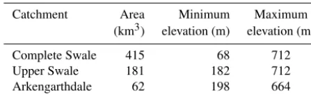
The basin studied is the River Swale in northern England. The mean basin relief is 357 m, ranging between 68 and 712 m with an average river gradient of 0.0064. The head-waters of the Swale are characterized by steep valleys and the geology is Carboniferous limestone and millstone grits (Bowes et al., 2003). Downstream, valleys are wider and less steep, with the underlying geology becoming Trias-sic mudstone and sandstones (Bowes et al., 2003). This basin has been extensively modelled in previous studies (Coulthard and Macklin, 2001; Coulthard and Van de Wiel, 2013; Coulthard et al., 2012b, 2013a), and a pre-calibrated version of the CAESAR-Lisflood model was readily avail-able. The basin was sub-divided to provide test subbasins of various sizes, giving three basin sizes – herein referred to as the complete Swale, the Upper Swale and the Arkengarthdale tributary (Fig. 1; Table 1).
2.3 Precipitation data and model configuration
Table 1.Basin areas and elevations for the three test basins used.
Catchment Area Minimum Maximum
(km3) elevation (m) elevation (m)
Complete Swale 415 68 712
Upper Swale 181 182 712
Arkengarthdale 62 198 664
with rainfall intensities in millimetres per hour. The maxi-mum available 10-year record was extracted from the period 2004–2014 for the 5 km cells lying over the Swale basin. The
0.25 h×5 km resolution were the finest-scale data available,
and to provide a range of different resolutions these data were resampled to the scales detailed below (Table 2). When ag-gregating to coarser spatial scales, the relative contribution of each 5 km cell was weighted, equal to its relative contri-bution to the basin. Therefore, with each spatial resolution the same volume rain input is applied at each daily time step. Note that this differs from some studies of the effect of spa-tial resolution, where some of the variation can be explained by producing rainfall records from a domain that exceeds the bounds of the basin. Here, only the spatial representation of the same rainfall record was examined.
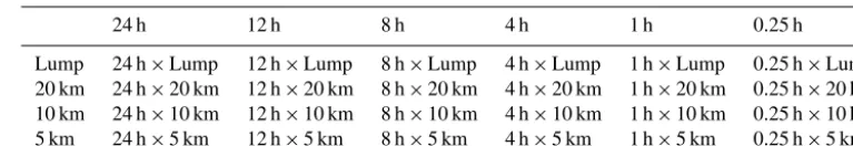
To study the absolute role of spatial and temporal precipi-tation data, a matrix of model runs was carried out as shown in Table 2. Spatially, rainfall was lumped into basin-average (henceforth “Lump”), 20, 10 and 5 km cells and temporally averaged into 24, 12, 8, 6, 4, 1 and 0.25 h time steps. This ma-trix of runs was applied to all three basins (complete Swale, Upper Swale and Arkengarthdale), though as the smallest basin (Arkengarthdale) is smaller than the 20 km resolution grid cell, it is run at 5 and 10 km and Lump spatial resolu-tions.
To investigate any longer-term impacts of precipitation resolution, two 1000-year simulations were carried out on the Upper Swale basin using the end members of our
driving data, the 24 h×Lump and 0.25 h×5 km resolution
data. Both simulations used the 10-year precipitation record looped 100 times. However, as this test would result in the same spatial patterns of rainfall being applied to the same area 100 times that could bias areas of erosion and deposi-tion to those receiving the most precipitadeposi-tion rather than be-ing a test of the spatial and temporal resolution. Therefore, to disrupt any spatial pattern legacies, two additional 1000-year simulations were carried out, where after every simu-lated 10 years, the locations of each rainfall pixel were ran-domly reassigned (called random 1 and random 2). Only two random simulations were carried out, due to long model run times and as these random runs gave very similar results. Re-sults from the two long-term simulations were then compared against both of these random simulations.
One aim of this research is to see whether any changes in sediment yields and erosion and deposition patterns due
to the spatial or temporal resolution of the precipitation could be accounted for by adjusting model parameters. To investigate this, three series of comparison runs were car-ried out, where a factor was added to the sediment trans-port model to allow erosion totals to be adjusted to match. This allowed us to normalize the sediment yields from the simulations being compared, with the aim of observ-ing any differences in spatial patterns of erosion and de-position in the DEMs. The following three sets of com-parisons of patterns of erosion and deposition were
car-ried out: for spatial resolution changes (0.25 h×Lump vs.
0.25 h×5 km), temporal-resolution changes (24 h×Lump
vs. 0.25 h×Lump), and spatial and temporal resolutions
(24 h×Lump vs. 0.25 h×5 km).
In order to adjust the sediment output, an additional term
or compensation factor C was added to the Wilcock and
Crowe (2003) sediment transport formula used here, as shown in Eq. (5) below (as fully described in Van De Wiel
et al., 2007). Here,qi is the sediment transport rate in square
metres per second,gis gravitational acceleration (m s−2),ρs
andρ are the density of sediment and water respectively,Fi
is the fractional volume of theith sediment in the top active
layer,U∗is the shear velocity (U∗=
τ/ρ0.5), andWi∗is a function that relates the fractional transport rate to the total transport rate.
qi=C
FiU∗3Wi∗ ((ρs−ρ)−1)g
(5)
For each of the three comparisons identified above (e.g.
24 h×Lump, 0.25 h×5 km and 0.25 h×Lump) runs were
carried out, varyingC from 1 to 2.5 in increments of 0.1,
resulting in an additional thirty 1000-year simulations. After this, the closest matching sediment yields over the 1000 years were used to compare differences in spatial patterns of ero-sion and deposition.
A final test was to determine whether changes in erosion and deposition were due to orographic effects. Previous re-search indicates a geomorphic sensitivity in the CAESAR model to rainfall magnitudes (Coulthard et al., 2012b), so it is therefore important to disentangle whether any increased erosion totals were due to the precipitation data resolution or orography. To test for this we carried out a series of
ad-ditional simulations using the 0.25 h×5 km data, where the
5 km rainfall grid cells were randomly redistributed or “jum-bled” to produce 20 different records. These jumbled data were then averaged to each of the temporal resolutions and the 30-year simulations were re-run.
Table 2.Matrix of runs using different temporal (x) and spatial (y) resolutions.
24 h 12 h 8 h 4 h 1 h 0.25 h
Lump 24 h×Lump 12 h×Lump 8 h×Lump 4 h×Lump 1 h×Lump 0.25 h×Lump 20 km 24 h×20 km 12 h×20 km 8 h×20 km 4 h×20 km 1 h×20 km 0.25 h×20 km 10 km 24 h×10 km 12 h×10 km 8 h×10 km 4 h×10 km 1 h×10 km 0.25 h×10 km 5 km 24 h×5 km 12 h×5 km 8 h×5 km 4 h×5 km 1 h×5 km 0.25 h×5 km
Table 3.CAESAR-Lisflood model parameters used.
CAESAR-Lisflood parameter Values
Grain sizes (m) 0.0005, 0.001, 0.002, 0.004, 0.008, 0.016, 0.032, 0.064, 0.128 Grain size proportions (total 1) 0.144, 0.022, 0.019, 0.029, 0.068, 0.146, 0.220, 0.231, 0.121 Sediment transport law Wilcock and Crowe (2003)
Max erode limit (m) 0.002 Active layer thickness (m) 0.01 Lateral erosion rate 0.0000005 Lateral edge smoothing passes 40
Metre value 0.01
Soil creep/diffusion value 0.0025 Slope failure threshold 45◦ Evaporation rate (m day−1) 0
Courant number 0.7
Mannings number 0.04
Table 4.Maximum rainfall intensities from the 10-year record for each resolution, taken from the domain for the complete Swale catchment.
using the 24 h×Lump rainfall. This “spinning up” process
removes sharp gradient changes in the DEM that may be a legacy of its generation and also allows the model to evolve a surface channel grain size distribution from the initial global distribution described in Table 3. Apart from rainfall param-eters and the basin DEM, all model paramparam-eters were kept constant, with one exception where the input–output
differ-ence allowed was set at 10 m3s−1 for the complete Swale,
5 m3s−1for the Upper Swale and 2.5 m3s−1for the
Arken-garthdale. This ensured that the model ran efficiently, with each value appropriate for the basin size and the hydrolog-ical regime. A list of CAESAR-Lisflood parameter values used in the simulations is shown in Table 3. The 1000-year simulations were carried out for the Upper Swale only, as the
longest run times here were 4 weeks compared to 8+weeks
for the whole Swale.
For all simulations, water and sediment outputs were sam-pled from the model at 0.25 h time steps and the DEM saved every 10 simulated years. From these data, mean annual out-put and values above the 95th percentile (representing peaks)
were calculated for both water (discharge rate m3s−1) and
sediment yield (m3). To allow better comparison between the
basin sizes, the above metrics were calculated as a percent-age deviation from the baseline, which was taken to be the
24 h×Lump resolution. To assess the impact of different
res-olutions on the modelled basin hydrology, outputs were com-pared to discharge data at Catterick Bridge using RMSE and Nash–Sutcliffe metrics for the 10-year record 2004–2014.
3 Results
3.1 Hydrology
ap-Table 5.The percentage deviations for each catchment of the mean annual hydrological outputs using different spatio-temporal resolu-tions.
Table 6.The percentage deviations for each catchment of the vol-ume of hydrological outputs above the 95th percentile using differ-ent spatio-temporal resolutions.
parent, with most differences linked to finer temporal reso-lutions. However, overall these changes are relatively minor (ca. 4 % for mean annual discharge and 5–10 % for peak dis-charges) especially when compared to the difference in max-imum rainfall intensity (Table 4).
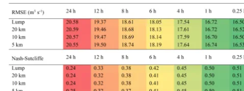
A full evaluation of hydrological performance could not be ascertained because the location of the nearest gauging sta-tion incorporates the contribusta-tion of a tributary outside of the modelled domain, though as this tributary was small in com-parison to the whole domain a relative comcom-parison could still be made. The relative comparisons showed that the change in resolution also influences the performance statistics for the hydrology with Table 7 showing an improvement in perfor-mance (RMSE and Nash–Sutcliffe) with finer temporal reso-lution, with only very small improvements due to finer spatial resolutions (RMSE only).
3.2 Sediment outputs
Tables 8 and 9 describe how with changing temporal and spa-tial resolution there is a clear trend of increasing sediment yields with finer spatial and temporal resolutions. Compared to basin hydrology, the results show that the sediment yield is notably more sensitive, with the greatest deviation being 118.1 % in the mean annual volumes, with the corresponding hydrological deviation being 2.8 %. Each basin shows a
sen-Table 7.Hydrological performance statistics from the Upper Swale catchment, comparing daily discharges from the CAESAR-Lisflood model and observed daily discharges recorded from Catterick Bridge. Red shading indicates the worst performance statistics and the green the best performance statistics.
Table 8.The percentage deviations for each catchment of the mean annual sediment yield outputs using different spatio-temporal reso-lutions.
sitivity to spatial resolutions, which increases with the basin size though differences are reduced between the 1 and 0.25 h temporal resolutions.
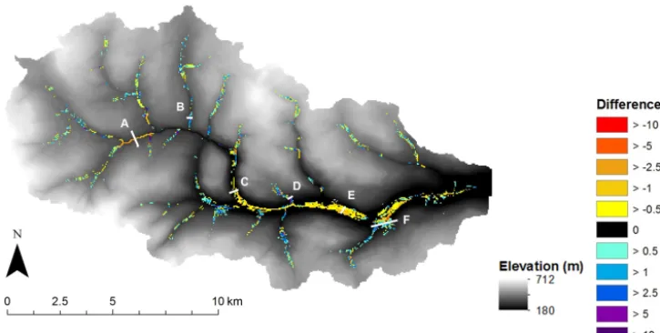
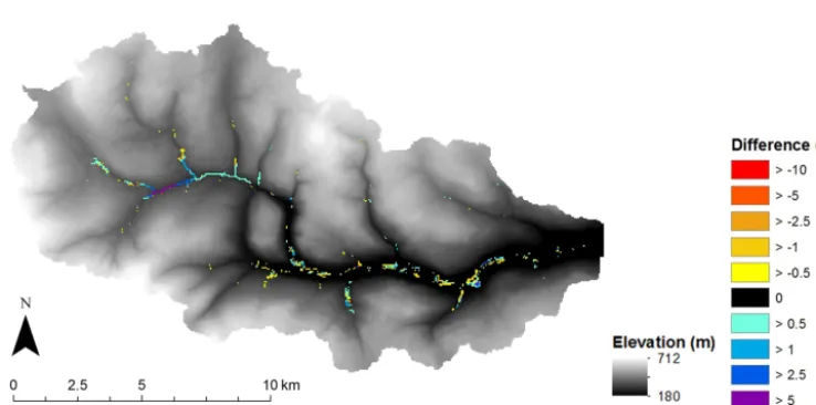
For the 1000-year simulations, there are differences in ero-sion and deposition patterns between the random 1 (with
0.25 h×5 km resolution data) and the 24 h×Lump
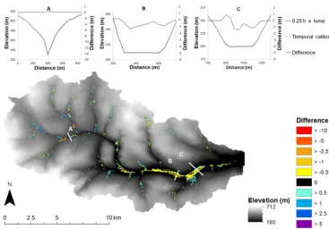
simula-tion (Fig. 2). Notably there is more erosion in all headwater and first-order streams and substantial amounts of deposition in the valley floors. The six cross sections (Fig. 3a to f) pro-vide more detail on morphological changes at these sites with a 3–5 m additional incision at cross section B and 6 m at cross section D, along with up to 3 m of deposition at cross sec-tions D and E. Interestingly, these are not restricted to single-channel threads; at E this occurs across some 350 m of val-ley floor. The results for the random 1 simulation were very similar to those for the random 2 simulation (not shown). However, there was a significant difference between random
1 and the 1000-year 0.25 h×5 km resolution simulation and
the random runs. These differences are a facet of repeating the 10-year rainfall sequence 100 times and are presented in Fig. 5, where the most notable difference is > 2.5 m in the val-ley floor to the western side of the basin along with smaller changes in the valley floor downstream.
For the 1000-year comparison runs, to account for the
simula-Figure 2.DEM of difference for the 1000-year Swale test. The differences shown are elevations from the 24 h×Lump simulation minus the elevations from the random 1 0.25 h×5 km. Cross sections (Fig. 3) are marked A–F. Yellows to reds indicate where the first (24 h×Lump) simulation has eroded more and deposited less than the second (random 1) simulation. Blues indicate more deposition and less erosion.
Table 9.The percentage deviations for each catchment of the vol-ume of sediment yield outputs above the 95th percentile using dif-ferent spatio-temporal resolutions.
tions gave sediment yields that were within 3 % of the
0.25 h×Lump simulation with a compensation factor of 2.0.
For spatial simulations, 0.25 h×Lump with a compensation
factor of 1.1 gave yields within 4 % of 0.25 h×5 km
simula-tions, and for spatial and temporal simulasimula-tions, 24 h×Lump
with a compensation factor of 2.2 was within 5 % of the
0.25 h×5 km simulation. Figures 6, 7 and 8 describe the
spa-tial patterns of the differences between the two final DEMs from these simulations. These show areas of greater differ-ence in the lower half of the basin for different temporal-resolution data, in the upper half of the basin for spatial res-olution data, and in both upper and lower halves for changes in spatial and temporal resolution. In each figure a series of cross sections are highlighted to illustrate vertical changes.
For the simulations to test the impact of orography, Fig. 9 shows there is a general, though not significant orographic relationship for rainfall intensity in the Swale. However, the results of the jumbled runs (Fig. 10) show that as the
tempo-Figure 3. Cross sections identified in tempo-Figure 2. 330 340 350 360 370 380
100 150 200 250 300
E lev a tio n ( m ) Distance (m) (a)
24 h × l ump Random 1 330 340 350 360 370 380
100 150 200 250 300
E lev a tio n ( m ) Distance (m) (b )
24 h × l ump Random 1 247 248 249 250 251 252 253 254 255
200 250 300 350 400
E lev a tio n ( m ) Distance (m) (c)
24 h × l ump Random 1 280 285 290 295 300 305 310
50 150 250
E lev a tio n ( m ) Distance (m) (d )
24 h × l ump Random 1 208 210 212 214 216 218 220
0 100 200 300 400
E lev a tio n ( m ) Distance (m) (e)
24 h × l ump Random 1 220 230 240 250 260 270 280
0 500 1000
E lev a tio n ( m ) Distance (m) (f)
24 h × l ump
Random 1
Figure 3.Cross sections identified in Fig. 2.
res-Figure 4.DEM of difference between 1000-year random runs 1 and 2.
Figure 5.DEM of difference (DOD) between 1000-year random 1 and the 0.25 h×5 km resolution simulation.
olution and not any orographic effects within the data that are responsible for the increased sediment yields described previously.
4 Discussion
4.1 The impact of precipitation spatial and temporal resolution on sediment yield and longer-term landscape evolution
Clearly, both the temporal and spatial resolution of precip-itation have an important effect on the amount of sediment coming from a basin and where it is eroded and deposited (Tables 8 and 9; Figs. 2 and 3). Finer-resolution (spatial and temporal) rainfall inputs can increase the local rainfall inten-sity over parts of the basin, whilst the overall rainfall vol-ume remains the same. This leads to a slight increase in the
Figure 6.DEM of difference for the adjusted temporal-resolution comparison. The differences shown are elevations from the 24 h×Lump (2.0 factor) simulation minus the elevations from the 0.25 h×Lump. Yellows to reds indicate where the first (24 h×Lump 2.0) simulation has eroded more and deposited less than the second (0.25 h×Lump) simulation. Blues indicate more deposition and less erosion.
Figure 8.DEM of difference for the adjusted temporal and spatial resolution comparison. The differences shown are elevations from the 24 h×Lump (2.2 factor) simulation minus the elevations from the 0.25 h×5 km. Yellows to reds indicate where the first (24 h×Lump 2.2) simulation has eroded more and deposited less than the second (0.25 h×5 km) simulation. Blues indicate more deposition and less erosion.
Figure 9. Relationship between the total rainfall and mean elevation for each 5 km pixel within the Complete Swale basin.
y = 7.5692x + 7966 R² = 0.4968
6000 8000 10 000 12 000 14 000 16 000
0 100 200 300 400 500 600
T o ta l r a in fa ll (m m )
Mean elevation (m)
-10 0 10 20 30 40 50 60 70
-7.5 -5 -2.5 0 2.5
Se di m en t Yie ld (% of 24 h our - Lum p ) 0.25 hour 1 hour 4 hour 6 hour 8 hour 12 hour 24 hour Linear (0.25 hour) Linear (1 hour) Linear (4 hour) Linear (6 hour) Linear (8 hour) Linear (12 hour) Linear (24 hour)
Figure 9.Relationship between the total rainfall and mean eleva-tion for each 5 km pixel within the complete Swale basin.
cross sections A and E). The disproportionate relationship between changes in hydrology and erosion and deposition is highly important in this context, as small changes in hy-drology (here local and temporal) can clearly have a signif-icant impact on basin sediment yield and local erosion and deposition patterns. This affirms the findings of Coulthard et al. (2012b), who noted the “geomorphic multiplier” effect between rain, runoff and sediment yield.
For existing and previous LEM studies, these results suggest that there may have been a systematic
under-Figure 9. Relationship between the total rainfall and mean elevation for each 5 km pixel within the Complete Swale basin.
y = 7.5692x + 7966 R² = 0.4968
6000 8000 10000 12000 14000 16000
0 100 200 300 400 500 600
T ot al Rain fall (m m )
Mean Elevation (m)
-20 -10 0 10 20 30 40 50 60 70
-7.5 -5 -2.5 0 2.5
S e d im en t yi el d ( % o f 2 4 h l u m p )
Hydrological output (% of 24 h lump)
0.25 h 1 h 4 h 6 h 8 h 12 h 24 h Linear (0.25 h) Linear (1 h) Linear (4 h) Linear (6 h) Linear (8 h) Linear (12 h) Linear (24 h)
× ×
Figure 10.The relationship between hydrological output and sed-iment yield from each temporal resolution, based on outputs of the 20 jumble ensembles of the Upper Swale catchment.
representation of basin-wide sediment yields by using lumped and coarse temporal-resolution climate/precipitation data. These is may not be of concern to many LEM studies, which are interested in exploring general relationships be-tween processes, drivers and subsequent landscape change. However, the spatial changes in erosion and deposition pat-terns generated by the different-resolution rainfall data will affect results and findings. Over the 1000 years we have sim-ulated in this study, the coarser-resolution data lead to more
incision/erosion in third-order and higher streams and less in first- and second-order streams. This has led to a change in the shape of the basin long profile and thus, when pro-jected over even longer timescales, will lead to changes in the shapes of predicted basins, landscapes and landforms. Resolving this is troublesome as for many existing models, especially those dealing with longer timescale simulations (e.g. > 10 000 years), incorporating high-resolution precipi-tation data is impractical. The data are simply not available, and generating synthetic rainfall is complex. Therefore, can these changes in erosion and deposition patterns (and sedi-ment yields) be compensated for via model adjustsedi-ment rather than calibration?
4.2 Adjusting to compensate for spatial and temporal rainfall resolution effects
In our final set of 1000-year comparison runs, erosion and deposition totals were adjusted so simulations with differ-ent spatial and temporal rainfall resolutions could be com-pared. Sediment yields could easily be matched; however, there were differences in erosion and deposition patterns pro-duced by different temporal (Fig. 6) and spatial resolutions (Fig. 7). This indicates that such adjustment (similar to that carried out by Willgoose and Riley, 1998) can be carried out but with some notable effects and possible limitations.
Adjusting for temporal changes in rainfall resolution led to good results in the upland, western side of the basin, with very few areas where there were differences in erosion and deposition patterns greater than 0.5 m (Fig. 6, cross section A). However, changes in the valley floor sections lower down are greater, with more erosion and less deposition generated by the adjusted 24 h resolution simulation (Fig. 6, cross sec-tions B and C). In the steeper upland areas a larger compen-sation factor (2.0) is required for the 24 h rainfall to gener-ate similar amounts of erosion as the more intense, flashier events from the 0.25 h data. As the 2.0 compensation factor is applied globally, in the lower parts of the basin where there is less difference in flow magnitudes generated by the 0.25 and 24 h runs, this leads to more erosion or less deposition.
Conversely, adjusting for spatial resolution leads to very small differences in the lower, eastern sections (Fig. 7, cross sections B and C) but major changes in the upland area with 8 m more erosion and less deposition from the adjusted Lump simulation in Fig. 7, cross section A. As for Fig. 2, by lump-ing local rainfall heterogeneity there are smaller flows in first- and second-order streams but greater flows in third-order ones – leading to the incision at cross section A. Here the incision at A is greater than values shown in Fig. 2 as the temporal resolution of the data is 0.25 h rather than 24 h. There are very few differences in the lower sections of the basin (Fig. 7, cross sections B and C) as for both simulations here the flows will be the sum of the total basin rainfall (as
rain cells are reassigned every 10 years in the 0.25 h×5 km
random simulation).
Adjusting for both (Fig. 8) best represents how most LEMs may be adjusted for using coarser spatial- and temporal-resolution data. This comparison required our largest com-pensation factor (2.2) and generated patterns that could be described as a merging of Figs. 6 and 7 – with more erosion and less deposition in cross sections A, B and C. As per the discussion for Fig. 2, the coarser-resolution data drives more erosion and less deposition in third-order streams and val-ley floor areas; if continued for more thousands of years, this would result in a considerably different long profile, which would change the morphometry of the basin.
There are further difficulties associated with adjusting models to compensate for different-resolution data. For
ex-ample, if we have a convective 4 h event of 6 mm h−1and a
synoptic 24 h event of 2 mm h−1, then adjusting erosion rates
for 24 h resolution data would scale erosion from the convec-tive storm down and the synoptic event up. This adjustment, however, would assume the same erosion–deposition rela-tionship between our synoptic and convective event, and in the context of climate change, it is highly likely that this will change. For example, climate changes may lead to more or less rainfall as well as greater or lesser rainfall durations and intensities. In other words, the relationship between mean annual erosion rates and mean annual rainfall is nonstation-ary, yet any calibrated adjustment or scaling factor is fixed to the properties of the period it was calibrated against. This could readily lead to “over-calibration”, a phenomenon noted by the hydrological community (Andréassian et al., 2012), where the parameters in hydrological models are adjusted too tightly based on too few observations. The issue of non-stationary calibration of parameters is also widely acknowl-edged in the hydrological modelling literature (for example, Beven, 2006) where the period simulated is far shorter, and therefore possibly less varied, than the longer timescales over which LEMs may operate.
In summary, the adjustment of model parameters can be used to compensate basin sediment yields for different-resolution rainfall data, but there is an impact on patterns of erosion and deposition within the basin. Using such adjust-ments is likely to be basin-specific and the correction will not be correct over changing climates. Calibration, the ad-justment of sediment yields to match field data, will likely encounter the same issues.
4.3 Are hydrological basin-wide metrics suitable for LEM/morphodynamic models?
predic-tion. Similar hydrographs of water and sediment at a basin exit may come from completely different parts – and leave a very different geomorphic signature. Here is an important distinction between the hydrology and geomorphology – as different hydrological responses will not necessarily leave any sort of hydrological record in the system. But geomor-phological changes in response to the hydrology will.
Largely, model metrics are driven by the aims of the model. For example, a hydrograph may be a very useful out-put for a basin hydrological model (to feed, for example, into a flood model), whereas for a morphodynamic model we are interested in the changes occurring throughout the basin, not just those reflected at the end. This is especially important for LEMs, where patterns of erosion and deposition feedback to control the shape of basins and landscape development – and this effect increases with the duration of model study or sim-ulation. This point is identified in recent work by Hancock et al. (2016), showing that using the SIBERIA model, over 10 000 years, different-shape landscapes can evolve yet gen-erate very similar sediment yields.
4.4 Limitations
It is important to consider that these findings are based on numerical simulations that contain many simplifications and assumptions. CAESAR-Lisflood is driven by a hydro-logical model where changes in land use are represented
through altering model parameters (m) leading to flashier or
more reduced hydrographs. This may prove to be a consid-erable sensitivity to precipitation temporal and spatial res-olution, and in these simulations we have deliberately used
a moderate value for an m of 0.01 – which in previous
CAESAR-Lisflood simulations has been used to represent natural scrubland. We would suggest that lower values for grassland (e.g. 0.005) would increase sensitivity and larger values for forest/woodland (0.02) would reduce sensitivity, though further simulations would be required to show this. Basin hydrology is a balance between precipitation, evapo-ration, infiltration and groundwater effects. These processes are all spatially and temporally variable, but we have quite deliberately only altered the rainfall to determine model sen-sitivity to just this parameter. Within CAESAR-Lisflood the
TOPMODEL mparameter is used to account for
evapora-tion, infiltration and groundwater effects and can also be changed spatially and temporally (Coulthard and Van De Wiel, 2016). Examining model sensitivity to both may be useful future research.
There may also be issues with the DEM resolution (here 50 m) and how that interacts with different spatial resolutions of rainfall inputs, with other researchers showing that grid res-olution in LEMs can have an impact (Hancock et al., 2016). Furthermore, there are uncertainties associated with the up-scaling of the precipitation data and the transfer of rain radar data to actual values. However, notwithstanding the above limitations, our results provide very useful insight into how
spatially and temporally changing precipitation can alter sim-ulated basin geomorphology and sediment yields.
5 Conclusions
Our findings show that simulated basin sediment yields and spatial patterns of erosion and deposition are sensitive to the spatial and temporal resolutions of precipitation data used to drive models. The impact of temporal changes is greater than that of spatial changes. Using finer-resolution data for both leads to significant increases in sediment
out-puts, with 0.25 h×5 km resolution data leading to a
dou-bling in basin sediment yields compared to the 24 h×Lump
data. These changes are due to finer-resolution data gen-erating increased erosion in upland and first-order streams with increased deposition and aggradation in valley floor areas. Further simulations indicated that the differences in total sediment yield could be removed with a compensa-tion/adjustment factor inserted in the sediment transport law. However, using such a factor resulted in notable differences in the topographies generated, especially in third-order and higher streams. Overall, the implications of these findings are that uncalibrated past and present LEMs using coarse spatial- and temporal-resolution precipitation drivers may be under-predicting basin sediment yields and under-predicting erosion in first-order streams but over-predicting erosion in third-order streams and valley floor areas. Calibrated LEMs may give correct sediment yields, but patterns of erosion and deposition will be different and the calibration may not be correct for changing climates. It is highly likely this will have significant impacts on the modelled basin profile and shape from long-timescale simulations. Our findings are placed in the context of LEMs – but it should be considered that such issues of rainfall spatial and temporal resolution may be highly important to soil erosion models and other basin-based sediment models that may be using coarser-resolution precipitation data.
Acknowledgements. The authors would like to thank the editors, the two reviewers and Declan Valters for their comments and suggestions, all of which contributed to greatly improving this paper. This work was funded by the NERC Flash Flooding from Intense Rainfall (FFIR) project, Susceptibility of Basins to Intense Rainfall and Flooding (SINATRA) NE/K008668/1.
Edited by: Gerard Govers
Reviewed by: two anonymous referees
References
Andréassian, V., Le Moine, N., Perrin, C., Ramos, M.-H., Oudin, L., Mathevet, T., Lerat, J., and Berthet, L.: All that glitters is not gold: the case of calibrating hydrological models, Hydrol. Process., 26, 2206–2210, doi:10.1002/hyp.9264, 2012.
Bates, P. D., Horritt, M. S., and Fewtrell, T. J.: A simple inertial formulation of the shallow water equations for efficient two-dimensional flood inundation modelling, J. Hydrol., 387, 33–45, doi:10.1016/j.jhydrol.2010.03.027, 2010.
Beven, K.: A manifesto for the equifinality thesis, J. Hydrol., 320, 18–36, doi:10.1016/j.jhydrol.2005.07.007, 2006.
Beven, K. and Hornberger, G.: Assessing the Effect of Spatial Pattern of Precipitation in Modeling Stream Flow Hydrographs1, Water Resour. Bull., 18, 823–829, doi:10.1111/j.1752-1688.1982.tb00078.x, 1982.
Beven, K. J. and Kirkby, M. J.: A physically based, vari-able contributing area model of basin hydrology/Un modèle à base physique de zone d’appel variable de l’hydrologie du bassin versant, Hydrol. Sci. Bull., 24, 43– 69, doi:10.1080/02626667909491834, 1979.
Bowes, M. J., House, W. A., and Hodgkinson, R. A.: Phosphorus dynamics along a river continuum, Sci. Total Environ., 313, 199– 212, doi:10.1016/S0048-9697(03)00260-2, 2003.
Bronstert, A. and Bárdossy, A.: Uncertainty of runoff mod-elling at the hillslope scale due to temporal variations of rain-fall intensity, Phys. Chem. Earth, Parts A/B/C, 28, 283–288, doi:10.1016/S1474-7065(03)00039-1, 2003.
Castelltort, S. and Van Den Driessche, J.: How plausible are high-frequency sediment supply-driven cycles in the stratigraphic record?, Sediment. Geol., 157, 3–13, doi:10.1016/S0037-0738(03)00066-6, 2003.
Coulthard, T. J. and Macklin, M. G.: How sensitive are river systems to climate and land-use changes? A model-based evaluation, J. Quaternary Sci., 16, 347–351, doi:10.1002/jqs.604, 2001. Coulthard, T. J. and Van De Wiel, M. J.: Quantifying fluvial non
linearity and finding self organized criticality? Insights from sim-ulations of river basin evolution, Geomorphology, 91, 216–235, doi:10.1016/j.geomorph.2007.04.011, 2007.
Coulthard, T. J. and Van de Wiel, M. J.: Climate, tectonics or mor-phology: what signals can we see in drainage basin sediment yields?, Earth Surf. Dynam., 1, 13–27, doi:10.5194/esurf-1-13-2013, 2013.
Coulthard, T. J. and Van De Wiel, M. J.: Modelling long term basin scale sediment connectivity, driven by spatial land use changes, Geomorphology, doi:10.1016/j.geomorph.2016.05.027, in press, 2016.
Coulthard, T. J., Kirkby, M. J., and Macklin, M. G.: Non-linearity and spatial resolution in a cellular automaton model of a small upland basin, Hydrol. Earth Syst. Sci., 2, 257–264, doi:10.5194/hess-2-257-1998, 1998.
Coulthard, T. J., Macklin, M. G., and Kirkby, M. J.: A cellular model of Holocene upland river basin and alluvial fan evolu-tion, Earth Surf. Proc. Land., 27, 269–288, doi:10.1002/esp.318, 2002.
Coulthard, T. J., Lewin, J., and Macklin, M. G.: Modelling differen-tial catchment response to environmental change, Geomorphol-ogy, 69, 222–241, doi:10.1016/j.geomorph.2005.01.008, 2005. Coulthard, T. J., Hancock, G. R., and Lowry, J. B. C.: Modelling
soil erosion with a downscaled landscape evolution model, Earth Surf. Proc. Land., 37, 1046–1055, doi:10.1002/esp.3226, 2012a.
Coulthard, T. J., Ramirez, J., Fowler, H. J., and Glenis, V.: Using the UKCP09 probabilistic scenarios to model the amplified im-pact of climate change on drainage basin sediment yield, Hy-drol. Earth Syst. Sci., 16, 4401–4416, doi:10.5194/hess-16-4401-2012, 2012b.
Coulthard, T. J., Neal, J. C., Bates, P. D., Ramirez, J., de Almeida, G. A. M., and Hancock, G. R.: Integrating the LISFLOOD-FP 2D hydrodynamic model with the CAESAR model: Implications for modelling landscape evolution, Earth Surf. Proc. Land., 38, 1897–1906, doi:10.1002/esp.3478, 2013a.
Coulthard, T. J., Ramirez, J. A., Barton, N., Rogerson, M., and Brücher, T.: Were rivers flowing across the Sahara during the last interglacial? Implications for human migration through Africa, PLoS One, 8, e74834, doi:10.1371/journal.pone.0074834, 2013b.
Einstein, H. A.: The bed-load function for sediment transport in open channel flows, in Technical Bulletin No. 1026, USDA Soil Conservation Service, vol. 1026, U.S. Department of Agri-culture, available at: http://books.google.com/books?hl=en&lr= &id=xIhtv2wpR9oC&pgis=1 (last access: 23 August 2012), p. 71, 1950.
Finnerty, B. D., Smith, M. B., Seo, D.-J., Koren, V., and Moglen, G. E.: Space-time scale sensitivity of the Sacramento model to radar-gage precipitation inputs, J. Hydrol., 203, 21–38, doi:10.1016/S0022-1694(97)00083-8, 1997.
Gabellani, S., Boni, G., Ferraris, L., von Hardenberg, J., and Provenzale, A.: Propagation of uncertainty from rainfall to runoff: A case study with a stochastic rain-fall generator, Adv. Water Resour., 30, 2061–2071, doi:10.1016/j.advwatres.2006.11.015, 2007.
Hancock, G. R. R., Coulthard, T. J. J., and Lowry, J. B. C. B. C.: Pre-dicting uncertainty in sediment transport and landscape evolution – the influence of initial surface conditions, Comput. Geosci., 90, 117–130, doi:10.1016/j.cageo.2015.08.014, 2016.
Hearman, A. J. and Hinz, C.: Sensitivity of point scale surface runoff predictions to rainfall resolution, Hydrol. Earth Syst. Sci., 11, 965–982, doi:10.5194/hess-11-965-2007, 2007.
Kouwen, N. and Garland, G.: Resolution considerations in using radar rainfall data for flood forecasting, Can. J. Civil. Eng., 16, 279–289, doi:10.1139/l89-053, 1989.
Krajewski, W. F., Lakshmi, V., Georgakakos, K. P., and Jain, S. C.: A Monte Carlo Study of rainfall sampling effect on a dis-tributed catchment model, Water Resour. Res., 27, 119–128, doi:10.1029/90wr01977, 1991.
Lague, D., Hovius, N. and Davy, P.: Discharge, discharge variabil-ity, and the bedrock channel profile, J. Geophys. Res.-Earth, 110, 1–17, doi:10.1029/2004JF000259, 2005.
Lobligeois, F., Andréassian, V., Perrin, C., Tabary, P., and Lou-magne, C.: When does higher spatial resolution rainfall in-formation improve streamflow simulation? An evaluation us-ing 3620 flood events, Hydrol. Earth Syst. Sci., 18, 575–594, doi:10.5194/hess-18-575-2014, 2014.
McMillan, H., Krueger, T., and Freer, J.: Benchmarking ob-servational uncertainties for hydrology: rainfall, river dis-charge and water quality, Hydrol. Process., 26, 4078–4111, doi:10.1002/hyp.9384, 2012.
82adec1f896af6169112d09cc1174499 (last access: 20 Septem-ber 2016), 2003.
Molnar, P., Anderson, R. S., Kier, G. and Rose, J.: Relationships among probability distributions of stream discharges in floods, climate, bed load transport, and river incision, J. Geophys. Res.-Earth, 111, 1–10, doi:10.1029/2005JF000310, 2006.
Nicótina, L., Alessi Celegon, E., Rinaldo, A., and Marani, M.: On the impact of rainfall patterns on the hydrologic response, Water Resour. Res., 44, 1–14, doi:10.1029/2007WR006654, 2008. Ogden, F. L. and Julien, P. Y.: Runoff model sensitivity to radar
rainfall resolution, J. Hydrol., 158, 1–18, doi:10.1016/0022-1694(94)90043-4, 1994.
Pessoa, M. L., Bras, R. L., and Williams, E. R.: Use of Weather Radar for Flood Forecasting in the Sieve River Basin: A Sensitiv-ity Analysis, J. Appl. Meteorol., 32, 462–475, doi:10.1175/1520-0450(1993)032<0462:uowrff> 2.0.co;2, 1993.
Segond, M. L., Wheater, H. S., and Onof, C.: The significance of spatial rainfall representation for flood runoff estimation: A nu-merical evaluation based on the Lee catchment, UK, J. Hydrol., 347, 116–131, doi:10.1016/j.jhydrol.2007.09.040, 2007. Simpson, G. and Castelltort, S.: Model shows that rivers transmit
high-frequency climate cycles to the sedimentary record, Geol-ogy, 40, 1131–1134, doi:10.1130/G33451.1, 2012.
Sólyom, P. B. and Tucker, G. E.: The importance of the catchment area-length relationship in governing non-steady state hydrol-ogy, optimal junction angles and drainage network pattern, Geo-morphology, 88, 84–108, doi:10.1016/j.geomorph.2006.10.014, 2007.
Tucker, G. E. and Bras, R. L.: A stochastic approach to modeling the role of rainfall variability in drainage basin evolution, Water Resour. Res., 36, 1953, doi:10.1029/2000WR900065, 2000. Tucker, G. E. and Hancock, G. R.: Modelling landscape evolution,
Earth Surf. Proc. Land., 35, 28–50, doi:10.1002/esp.1952, 2010.
Tustison, B., Harris, D., and Foufoula-Georgiou, E.: Scale issues in verification of precipitation forecasts, J. Geophys. Res.-Atmos., 106, 11775–11784, doi:10.1029/2001JD900066, 2001.
Wainwright, J. and Parsons, A. J.: The effect of temporal variations in rainfall on scale dependency in runoff coefficients, Water Re-sour. Res., 38, 7-1–7-10, doi:10.1029/2000WR000188, 2002. Welsh, K. E., Dearing, J. A., Chiverrell, R. C., and Coulthard,
T. J.: Testing a cellular modelling approach to simulating late-Holocene sediment and water transfer from catchment to lake in the French Alps since 1826, Holocene, 19, 785–798, doi:10.1177/0959683609105303, 2009.
Van De Wiel, M. J. and Coulthard, T. J.: Self-organized criticality in river basins: Challenging sedimentary records of environmental change, Geology, 38, 87–90, doi:10.1130/G30490.1, 2010. Van De Wiel, M. J., Coulthard, T. J., Macklin, M. G., and Lewin,
J.: Embedding reach-scale fluvial dynamics within the CAESAR cellular automaton landscape evolution model, Geomorphology, 90, 283–301, doi:10.1016/j.geomorph.2006.10.024, 2007. Wilcock, P. R. P. and Crowe, J. J. C.: Surface-based transport
model for mixed-size sediment, J. Hydraul. Eng., 129, 120–128, doi:10.1061/(ASCE)0733-9429(2003)129:2(120), 2003. Willgoose, G.: User Manual for Siberia (version 8:30), July, 115,
http://csdms.colorado.edu/w/images/SIBERIA_8.30_Manual. pdf (last access: 22 September 2016), 2005.
Willgoose, G. and Riley, S.: The long-term stability of engi-neered landforms of the Ranger Uranium Mine, Northern Ter-ritory, Australia: Application of a catchment evolution model, Earth Surf. Proc. Land., 23, 237–259, doi:10.1002/(SICI)1096-9837(199803)23:3<237::AID-ESP846>3.0.CO;2-X, 1998. Wilson, C. B., Valdes, J. B., and Rodriguez-Iturbe, I.: On the