Atmos. Meas. Tech., 5, 831–841, 2012 www.atmos-meas-tech.net/5/831/2012/ doi:10.5194/amt-5-831-2012
© Author(s) 2012. CC Attribution 3.0 License.
Atmospheric
Measurement
Techniques
How to average logarithmic retrievals?
B. Funke1and T. von Clarmann2
1Instituto de Astrof´ısica de Andaluc´ıa, CSIC, Granada, Spain
2Karlsruhe Institute of Technology, Institute for Meteorology and Climate Research, Karlsruhe, Germany
Correspondence to: B. Funke ([email protected])
Received: 18 November 2011 – Published in Atmos. Meas. Tech. Discuss.: 5 December 2011 Revised: 10 April 2012 – Accepted: 11 April 2012 – Published: 25 April 2012
Abstract. Calculation of mean trace gas contributions from profiles obtained by retrievals of the logarithm of the abun-dance rather than retrievals of the abunabun-dance itself are prone to biases. By means of a system simulator, biases of linear versus logarithmic averaging were evaluated for both maxi-mum likelihood and maximaxi-mum a priori retrievals, for various signal to noise ratios and atmospheric variabilities. These bi-ases can easily reach ten percent or more. As a rule of thumb we found for maximum likelihood retrievals that linear aver-aging better represents the true mean value in cases of large local natural variability and high signal to noise ratios, while for small local natural variability logarithmic averaging often is superior. In the case of maximum a posteriori retrievals, the mean is dominated by the a priori information used in the retrievals and the method of averaging is of minor con-cern. For larger natural variabilities, the appropriateness of the one or the other method of averaging depends on the par-ticular case because the various biasing mechanisms partly compensate in an unpredictable manner. This complication arises mainly because of the fact that in logarithmic retrievals the weight of the prior information depends on abundance of the gas itself. No simple rule was found on which kind of averaging is superior, and instead of suggesting simple recipes we cannot do much more than to create awareness of the traps related with averaging of mixing ratios obtained from logarithmic retrievals.
1 Introduction
Retrieval of mixing ratios or concentrations of atmospheric trace species from remote radiance or transmission measure-ments involves inverse modelling of radiative transfer. In or-der to avoid to retrieve negative thus unphysical mixing ratios
of trace species, to better cope with the large dynamical range of possible values, or to better reflect the assumed natural distribution of the species under assessment, often the log-arithm of the concentration is retrieved instead of the con-centration itself (e.g. von Clarmann et al., 2009; Funke et al., 2009; Papandrea et al., 2005; Bowman et al., 2006; Schneider et al., 2006; Urban et al., 2005). While negative concentra-tions certainly are unphysical, their removal by the logarith-mic retrieval may bias averages of retrieved concentrations high due to the asymmetric error propagation. In this paper we assess if it is appropriate to average results in the loga-rithmic domain in order to reduce these biases. This analysis is done by means of a system simulator which propagates signal and noise through an idealized retrieval and which is described in Sect. 2. In Sect. 3 we analyze related case stud-ies, and in Sect. 4 we give recommendations which kind of averaging is advisable in which context and critically discuss to which degree the conclusions of this study can be gen-eralized towards a wider range of applications beyond the idealized cases analyzed in this paper.
2 The system simulator
use a modeled distribution of atmospheric concentrations as reference ensemblex of concentrationsxn,n=1,. . . N, ex-pressed as volume mixing ratios (vmrs). The vmr histograms of these distributions were found to resemble a wide range of probability density functions, e.g. normal when the standard deviation is much smaller than the mean, log-normal when the standard deviation is large compared to the mean, or bi-modal when the averaged ensemble contains two “favorite” atmospheric conditions.
For each concentrationxn, the related measurement signal
ynis simulated as
yn=y0+kxn+n, (1)
wherey0is a constant background signal,kis the sensitivity dy/dx of the measurement system and n is the measure-ment error associated with thenth measurement. The latter is obtained from a pseudo-random number generator provid-ing normally distributed random numbers of zero expectation and variances2.
Without loss of generality, we sety0=0 andk=1. The measurement variance is then set tos2= ¯x2/r2, wherex¯ is the mean value of the concentrationsxn andr is a tunable average signal to noise ratio (SNR).
The simulated measurements yn are then propagated through an iterative retrieval simulator operating in the ln(vmr) domain. With
dyn d lnxn
=k dxn
d lnxn
=xn (2)
we have for iterative unconstrained maximum likelihood retrievals
lnxn,i+1=lnxn,i+xn,i−1(yn−xn,i) , (3) wherexi,nis the concentration retrieved in theith iteration from thenth simulated measurement. For positive signalsyn, Eq. (3) converges towardsxn,I=xn+n, whereI denotes the final iteration of sample n and n is the measurement error propagated into the x-space, as in the case of linear maximum likelihood retrievals.
For maximum a posteriori (optimal estimation) retrievals (Rodgers, 2000), we have
lnxn,i+1=lnxn,i +
xn,i
s2 (yn−xn,i)−σa−2(lnxn,i−lnxa)
σa−2+xn,i2 s−2
(4)
wherexa is the prior information onx with varianceσa2 in the logarithmic domain. Since biases caused by inappropriate prior information and variance are beyond the scope of this study, we make two further idealizing assumptions,
xa=exp "PN
n=1lnxn
N
#
(5)
and
σa2= PN
n=1(lnxn−lnxa)2
N , (6)
i.e. assuming that the a priori information and its variance are equal to the arithmetic mean and standard deviation, re-spectively, of the “true” distribution in the logarithmic do-main. This would be the optimum condition for a maxi-mum a posteriori retrieval, although difficult to achieve in real applications since the true state of the atmosphere is un-known and not necessarily represented by the climatological distribution.
As a variation of this scheme, we have also performed simulations with a constant a priori varianceσa2=ln 2, cor-responding to a 100 % variance in the linear space. This is motivated by the lack of reliable information on climatolog-ical variances in real applications. A 100 % variance is thus often assumed in optimal estimation schemes applied to re-mote sensing data. The rationale for choosing this value is to reduce the a priori content of the results while guaranteeing reasonable and stable retrievals. In the following, we refer to this ad hoc variant of optimal estimation as “modified” maximum a posteriori approach.
Convergence of the iterative retrieval scheme is reached when the absolute difference of lnxn,i+1 and lnxn,i is smaller than 0.001σx, i.e. a fraction of the estimated retrieval noise error in the logarithmic retrieval space, which can be expressed usingk=1 by
σx=
s xn,i
x2n,i+s2σ−2 a
, (7)
with σa−2=0 for maximum likelihood retrievals, σa−2= 1/(ln 2)for modified maximum a posteriori retrievals, and
σa−2inferred from the actual variability of the true state in the logarithmic domain for Bayesian maximum a posteriori retrievals.
B. Funke and T. von Clarmann: How to average logarithmic retrievals 833
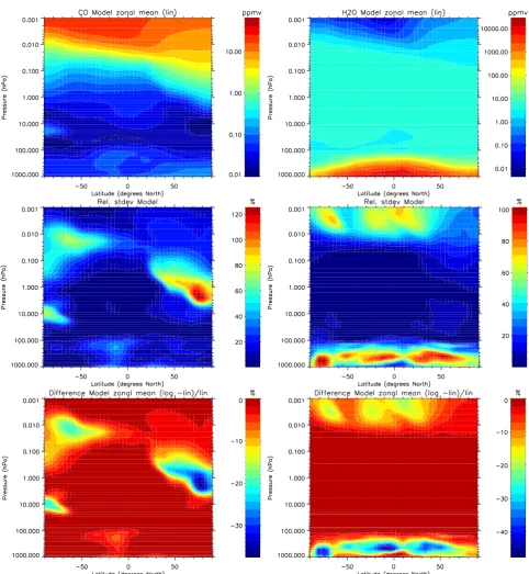
Fig. 1. Model zonal mean distributions of zonal mean vmrs (top), standard deviations (middle), and differences between linear and
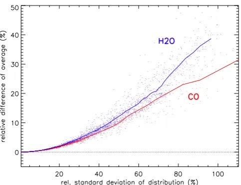
Fig. 2. Differences of linearly and logarithmically averaged zonal
means (relative to linearly averaged zonal means) versus standard deviation of the distributions for CO (red) and H2O (blue). Data points represent single latitude/altitude boxes.
The assessment of averaging procedures is then based on the comparison ofN−1PNn=1xn,I toN−1PNn=1xn and
N−1PNn=1lnxn,I toN−1PNn=1lnxn, respectively. Compar-ison of like with like certainly is idealistic, because in prac-tice climatological data are often compared among each other without questioning how the climatologies have been gener-ated. Nevertheless, we think that comparison of logarithmic averages of logarithmic retrievals with linear averages of the true state would not be fair.
It is evident that averages of maximum a posteriori re-trievals depend on the a priori information. A more rigorous approach is thus to compare to averages of
˜
xn=exp [Anln(xn)+(1−An)ln(xa)], (8) with the averaging kernel
An=
xn,I2 xn,I2 +s2σ−2
a
. (9)
˜
xn is the retrieval response to the “true” state xn (i.e. the retrieval result for=0, i.e. no measurement noise consid-ered). Note that 1−Andescribes also the a priori contribution to the solutionxn,I which, contrary to the case of linear re-trievals, depends on the solution itself. This approach is com-monly used in point-to-point comparisons of remotely sensed data with model results or independent measurements. How-ever, in many averaging applications (i.e. comparisons of trace gas climatologies), averaging kernels of individual en-semble members are not available. For this reason, we com-pare to averages of bothx˜nandxnin the case of maximum a posteriori retrievals.
While averaging of maximum a posteriori retrievals with-out re-adjustment of the content of a constant priori in-formation is questionable because the optimal mean is not
identical to the mean of optimal estimates (Rodgers, 2000, Chap. 10.4.1), and because prior knowledge of a single at-mospheric state is less reliable than priori knowledge on the mean atmospheric state, we ignore the re-adjustment of the a priori content to produce an optimal average, because this is rarely done in practice and beyond the scope of this paper.
3 Case studies
The case studies are organized in a way that first uncon-strained maximum likelihood retrievals and then standard and modified maximum a posteriori retrievals are discussed. For each of these retrieval schemes we perform simulations for different SNRs covering values from 0.5 to 10.
In order to provide realistic examples, the ensemblesxn represent zonal distributions of CO and H2O taken from WACCM model simulations described in Jackman et al. (2008) for the period of November 2003 in a vertical range from 1000–0.001 hPa with global latitudinal coverage. For each altitude-latitude gridpoint of the model (gridwidth 4.5◦ in latitude, and 55 pressure gridpoints between 103 and 10−3hPa), we get a distribution composed of about 10 000 different zonal and temporal model values for each species. Concentrations of CO and H2O are retrieved in the ln(vmr) space in many atmospheric remote sensing applications (e.g. von Clarmann et al., 2009; Funke et al., 2009; Schneider et al., 2006; Deeter et al., 2007). The global distribution of the corresponding averages (i.e. zonal means) is shown in Fig. 1 (top).
Highest standard deviationsσm of the modeled distribu-tions are found where spatial gradients are strongest, i.e. in regions of transport barriers, vertical transport, etc. In the case of CO, this occurs in the polar regions in the mid-stratosphere and is related to vertical transport by the merid-ional circulation. H2O variability is highest in the UTLS (see Fig. 1, middle). These standard deviations represent the local natural variability of the atmospheric state, as opposed to any scatter being caused by measurement noise.
The magnitudes of differences of linear and logarithmi-cally averaged zonal means correlate spatially with the stan-dard deviation of the distributions for both CO and H2O (Fig. 1, bottom). This correlation is quite compact (see Fig. 2). The differences between linear and logarithmic aver-aging are somewhat more pronounced for H2O than for CO. For a local natural variability of 100 % in terms of standard deviation, the differences reach 40 % for H2O but only 30 % for CO.
3.1 Maximum likelihood retrievals
B. Funke and T. von Clarmann: How to average logarithmic retrievals 835
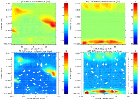
Fig. 3. Zonal mean differences of retrieved and “true” distributions (relative to the latter) for CO (left) and H2O (right). Top: linear averages, bottom: logarithmic averages. Results are shown for maximum likelihood ln(vmr)-retrieval simulations with a signal to noise ratio of 2. White regions in the lower panels reflect unreasonable results (“zero” averages, see text for further explanations).
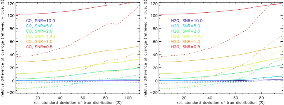
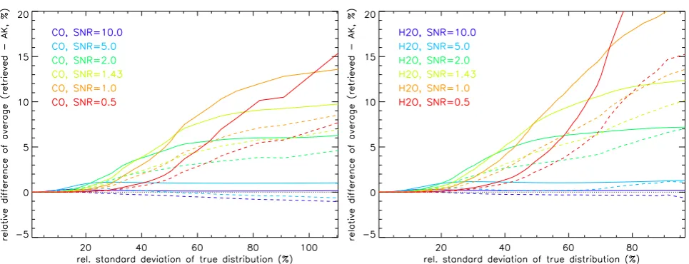
Fig. 4. Differences of retrieved and “true” zonal means (relative to the latter) versus local natural variability in terms of standard deviation
Fig. 5. Differences of retrieved and “true” zonal means (relative to the latter) versus local natural variaility in terms of standard deviation
for the CO (left) and H2O (right). Solid: linear averages, dashed: logarithmic averages. Results are shown for maximum likelihood ln(vmr)-retrieval simulations with signal to noise ratios of 10 (dark blue), 5 (light blue), 2 (dark green), 1.43 (light green), 1.0 (orange), and 0.5 (red).
signals, the logarithmic maximum likelihood retrieval yields the same result as the retrieval in the linear domain. How-ever, the rejection of unconverged logarithmic retrievals with a negative signal from the averages leads to positive bias compared to averaged results retrieved in the linear domain.
As a consequence, linear averages of logarithmic retrievals are biased high compared to the corresponding averages of the “true” distribution. For a constant SNR, this bias is cor-related with the dispersion of the “true” ensemble. Assuming a SNR of 2, the bias between the retrieved and the true zonal mean distributions of CO and H2O varies from 2 % to 25 %, being highest in regions with most pronounced atmospheric variability (see Fig. 3, upper panels).
In the case of logarithmic averaging, this behavior is partly compensated by the asymmetric mapping of the normal-distributed noise into the ln(vmr) parameter space, introduc-ing a negative bias compared to the correspondintroduc-ing averages of the “true” distributions. This negative bias dominates for low atmospheric variability. Figure 3 (lower panels) shows this behavior for a SNR of 2. Here, the overall bias between retrieved and true zonal mean distributions of CO and H2O varies from−15 % to 30 % in dependence of the “true” dis-tributions’ dispersion.
Interestingly, logarithmically averaged retrievals of some particular latitude/altitude boxes become virtually zero. This random-like behavior is introduced by single retrievals of signals being infinitesimally close to zero, leading to high negative values in the ln(vmr) space. The occurrence of such artifacts is ruled by the probability density of such small sig-nals which, in turn, is linked to the variance of the measure-ment noise. For high SNR, this probability density is small, because the relevant interval of signals is located on the tail of the Gaussian distribution. It is also small for low SNR,
because due to the broader probability distribution function most negative signal values are so negative that the retrieval does not reach convergence and related results are discarded, and only very few measurements hit the small interval where the measurements are negative to cause problems but their absolute values are small enough to still allow convergence. Most frequent occurrences of this peculiarity are found for intermediate SNRs of around 2.
Figure 4 shows the relative differences between retrieved and “true” averages as function of the relative standard de-viation of “true” distribution σm for a SNR of 2, summa-rizing the behavior discussed above. The correlation of dif-ferences and the local natural variability is quite compact. Therefore, in the following we restrict our analysis to its average dependence (indicated by solid lines in Fig. 4).
It is interesting to notice that, in the case of H2O distri-butions, the dependence onσmis more pronounced for loga-rithmic than for linear averages, while this is not the case for CO. This is most likely related to differences in the shapes of the PDFs of both species in regions with high local natural variability.
Figure 5 summarizes the results for maximum likelihood retrievals for a variety of SNRs. In general, linear averag-ing is superior in the case of high SNR and large local nat-ural variability, while logarithmic averaging is superior in the case of small SNR and small natural variability, although exceptions exist.
B. Funke and T. von Clarmann: How to average logarithmic retrievals 837
pronounced low bias of logarithmic averages was introduced due to the increased contribution of very small values ofxn,I. The latter depends then strongly on the choice of the maxi-mum number of iterations or on the choice of the fake value, respectively. In our case (maximum number of iterations of 20), the inclusion of these retrieval results would introduce a low bias of logarithmic averages of up to 70 % for low SNR, completely disabling its meaningful interpretation.
3.2 Maximum a posteriori retrievals
The same kind of analysis also has been performed for max-imum a posteriori retrievals. Comparisons of the linear and logarithmic averages with the “true” averages as a function of natural variability are shown in Fig. 6 for various signal to noise ratios. In the case of low local natural variability – and thus also low a priori variance – the differences are small because the content of a priori information in the retrieval is large. As already mentioned in Sect. 2, averaging of re-trievals containing a constant prior information does not pro-duce an optimal average, since the prior information is sys-tematically overrepresented in the mean. On the other hand, the prior information characterizes the mean state of the at-mosphere better than an actual state. The problem of the need of re-adjustment of the weight of the priori information in the mean, however, is beyond the scope of this study.
For intermediate local natural variability and a priori vari-ance, linear averages of logarithmically retrieved mixing ra-tios are biased low. This is, because the a priori state of the atmosphere is calculated by logarithmic averaging of the true distribution. This low bias is not more than the bias between the logarithmic and linear averages of the “true” distribution, which is, via the content of priori information in the retrieval, propagated to the averages of the retrievals. Results for less ideal a priori information may be different. In the case of large local natural variability along with large a priori vari-ance, the bias of the linear average turns high, similar to the case of maximum likelihood retrievals but with a consider-ably smaller amplitude (less than 5 % even for low SNRs). The positive bias of maximum a posteriori retrieval averages, however, is not related to the rejection of unconverged re-trievals of negative signals (convergence is in our simplified one-dimensional retrieval always achieved due to the con-straint), but to the dependence of the a priori contribution to the retrieval solution on the solution itself (see Sect. 2). That is, retrievals of low signals (either due to low values ofxn or negative values ofn) have a higher a priori contribution than those of high signals, resulting in a high bias. The turn-ing point, i.e. where the high bias due to asymmetric a priori mapping starts to overcompensate the low bias introduced byxaitself, depends strongly on the SNR. For SNRs greater than 5, differences start to increase already at standard devi-ations below 20 %, while for SNRs lower than 1 the turning point is located at standard deviations greater than 50 %.
Logarithmic averages of logarithmic maximum a posteri-ori retrievals are generally higher than the logarithmic aver-ages of the “true” distribution for intermediate to high val-ues ofσm(i.e. when there is a substantial contribution of the measurement to the retrieval solution). Contrarily to the lin-ear averaging case, no negative bias due to the a priori con-tribution is introduced since, in our idealized case, the prior information is identical the the “true” logarithmic average. Logarithmic averaging performs apparently worse compared to linear averaging for high values ofσm. This, however, is related to the compensation effect of the a priori in the linear averaging (see discussion above) and hence depends strongly on the choice of the a priori.
In addition, we have also compared the linear and log-arithmic averages to the averaged linear retrieval response to the “true” distributionxn, the latter obtained by applying the averaging kernelsAn(Rodgers, 2000) toxnaccording to Eq. (8) (see Fig. 7). In first order, these comparisons show the isolated effect of the asymmetric mapping of noise in the constrained retrieval, that is, the influence of the a pri-ori information on the difference between the retrieved and the “true” mean, is removed. Now, the bias between linear averages of the retrieval results and the linear retrieval re-sponse to the “true” distribution is generally positive. This high bias is increased compared to Fig. 6 since the compen-sation effect of the a priori contribution is removed. For loga-rithmic averages, these differences are smaller. The generally better performance of logarithmic averages is related to the compensation of the positive bias due to the dependence of the a priori contribution onxn,I by the negative bias caused by asymmetric mapping of normal-distributed noise in the ln(vmr) space. The latter dominates for high SNRs, giving raise to a negative overall bias of logarithmic averages for SNRs greater than 5 in Fig. 7.
In summary, except for high SNRs (>5), logarithmic aver-aging of logarithmic maximum a posteriori retrievals is rec-ommended in validation exercises or point-to-point model-data comparisons whenever averaging kernels related to in-dividual measurements are applied to the corresponding data to be compared.
3.3 Modified a posteriori retrievals
Since in practical applications of the optimal estimation re-trieval scheme often ad hoc choices of a priori variances are made, we also have studied averaging of logarithmic re-trievals where the a priori standard deviation was set to 100 % (see Fig. 8). For high value ofσm, the behavior is similar to the classical maximum a posteriori retrievals (Fig. 7). For lower values ofσm, however, the measurement contribution to the retrieval solution is much higher than in the classical maximum a posteriori case and differences of retrieved and “true” averages are increased.
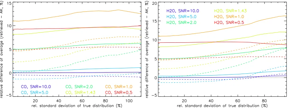
Fig. 6. Differences of retrieved and “true” zonal means (relative to the latter) versus local natural variability in terms of standard deviation
for the CO (left) and H2O (right). Solid: linear averages, dashed: logarithmic averages. Results are shown for maximum a posteriori ln(vmr)-retrieval simulations with SNRs of 10 (dark blue), 5 (light blue), 2 (dark green), 1.43 (light green), 1.0 (orange), and 0.5 (red). Note that the a priori contribution to the retrievals is greater than 50 % for standard deviations below 10 %, 20 %, 50 %, 70 %, 100 %, and 200 %, respectively.
Fig. 7. Differences between the mean values and the mean “true” atmospheric state after application of the averaging kernel to the latter for
B. Funke and T. von Clarmann: How to average logarithmic retrievals 839
Fig. 8. Differences of retrieved and “true” zonal means (relative to the latter) versus local natural variability in terms of standard deviation
for the CO (left) and H2O (right). Solid: linear averages, dashed: logarithmic averages. Simulations are performed with a modified maximum a posteriori ln(vmr)-retrieval simulations using a fixed constraint corresponding to climatological variance of 100 %. Results for signal to noise ratios of 10 (dark blue), 5 (light blue), 2 (dark green), 1.43 (light green), 1.0 (orange), and 0.5 (red) are shown. The resulting a priori contributions are 1 %, 3.8 %, 20 %, 33 %, 50 %, and 80 %, respectively.
Fig. 9. Differences of retrieved and linear retrieval response (i.e. averaging kernels applied to the “true” profiles) zonal means (relative to
distribution xn (see Fig. 9) shows that the use of a con-stant a priori variance removes the dependence of the biases onσm and they remain approximately constant. Again, bet-ter performance is achieved with logarithmic averaging for SNR<5 due to the compensation of the positive bias due to the dependence of the a priori contribution on xn,I by the negative bias caused by asymmetric mapping of normal-distributed noise in the ln(vmr) space. For higher SNRs, how-ever, linear averaging yields smaller biases.
4 Conclusions
Ideally, the average of concentration shall be mass-conservative in a sense that the average concentration times the airmass equals the total amount of the target gas in the air-mass. This can only be achieved with linear averaging. Both linear and logarithmic averaging of logarithmic retrievals can lead to biases of several ten percent, which are typically larger for larger local atmospheric variability. Biases caused by the impossibility of logarithmic retrievals of mapping neg-ative measured signals into the atmospheric state space can be remedied by neither of the averaging schemes.
Usually, for maximum likelihood retrievals linear averag-ing better represents the true mean value in cases of large local natural variability and high signal to noise ratios, while for small local natural variability logarithmic averaging of-ten is superior. For maximum a posteriori retrievals, the de-pendence of the weight of the priori information on the state value itself causes an unpredictable interaction between the effect of the constraint on the retrieval and the characteristics of the averaging procedure. Since in logarithmic retrievals the prior information is ideally chosen as the expectation value of the logarithm of the atmospheric state variable, log-arithmic averaging of results better reproduces the logarith-mic average of the true atmospheric state in cases when the retrieval is dominated by the prior information. For higher atmospheric variability, which in a truly Bayesian maximum a posteriori retrieval goes along with a lesser weight of prior information, the bias of the average is composed of the super-position of the effects of multiple biasing processes of posi-tive and negaposi-tive sign. The assumption that the prior informa-tion is identical with the true local mean of the atmospheric state is certainly an ideal case and more realistic cases where the a priori information differs from the true mean state of the atmosphere may lead to even different results but could not be assessed here.
Further, these investigations refer to an ideal world where logarithmic averages of logarithmic retrievals are compared to logarithmic averages of the true atmospheric state values. In the real world, however, the user of climatologies may not ask about the procedure how a climatology has been gener-ated and may unintentionally compare a climatology based on logarithmic averages of logarithmic retrievals from one instrument with linear averages of linear retrievals of another
instrument, which adds an additional bias of up to 40 % (see Fig. 2).
In summary, averaging of logarithmically retrieved abun-dances of atmospheric species contains a lot of traps which cannot be avoided by application of a simple recipe. Partic-ularly, biasing can never be systematically avoided by using a superior averaging scheme. At best, limitation of damage can be aimed at. While logarithmic averaging in some cases indeed performs better than linear averaging, particularly in some cases of Bayesian or modified maximum a priori re-trievals, related biases are by no means fully compensated.
Although our simulations have been carried out for an one-dimensional retrieval problem under the idealized assump-tion of locally linear radiative transport, the conclusions of this study can be generalized in a qualitative manner to more realistic retrieval problems. For example, multi-dimensional profile retrievals, typically performed in remote sensing ap-plications, would suffer the same problems as described here with the added complexity of correlations between different profile points. These correlations are typically introduced by instrumental and/or geometrical limitations in vertically re-solving the profiles, i.e. the line of sight of a remote sounder travels through multiple atmospheric layers. Thus a single measurement error cannot be assigned to a single profile point but to positively or negatively correlated errors at vari-ous altitudes. Inclusion of constraints (e.g. maximum a pos-teriori retrievals) further contributes to these correlations.In a similar way, our results are, in a qualitative sense, also valid for multi-species retrievals. Quantitative results for such ap-plications, however, depend on the particular case anyway.
The inclusion of non-linear radiative transport would not alter the presented results for unconstrained maximum like-lihood retrievals, however, results for maximum a posteriori retrieval averages might differ due to an amplification (or re-duction) of the positive bias related to the dependence of the a priori contribution to the retrieval solution on the solution itself. The latter effect, as described in Sect. 3.2, is already caused by the “artificial” non-linearity introduced by the re-trieval of ln(vmr). Additional non-linearity related to radia-tive transfer leads only to its modification. In consequence, we also expect biases related to the dependence of the a priori contribution to the retrieval solution on the solution itself in the case of averaging linear maximum a posteriori retrievals whenever non-linear radiative transfer occurs or, if the ob-served signal depends on additional quantities (e.g. tempera-ture in the case of emission measurements) being correlated to the retrieval quantity.
Acknowledgements. The authors like to thank the Toronto SPARC
B. Funke and T. von Clarmann: How to average logarithmic retrievals 841
providing WACCM model results. BF was supported by by the Spanish MICINN under project AYA2008-03498/ESP and project 200950I081 of CSIC.
Edited by: P. Eriksson
References
Bowman, K. W., Rodgers, C. D., Kulawik, S. S., Worden, J., Sarkissian, E., Osterman, G., Steck, T., Lou, M., Eldering, A., Shephard, M., Worden, H., Lampel, M., Clough, S., Brown, P., Rinsland, C., Gunson, M., and Beer, R.: Tropospheric Emis-sion Spectrometer: Retrieval Method and Error Analysis, IEEE T. Geosci. Remote, 44, 1297–1307, 2006.
Deeter, M. N., Edwards, D. P., and Gille, J. C.: Retrievals of carbon monoxide profiles from MOPITT observations using lognormal a priori statistics, J. Geophys. Res., 112, D11311, doi:10.1029/2006JD007999, 2007.
Funke, B., L´opez-Puertas, M., Garc´ıa-Comas, M., Stiller, G. P., von Clarmann, T., H¨opfner, M., Glatthor, N., Grabowski, U., Kell-mann, S., and Linden, A.: Carbon monoxide distributions from the upper troposphere to the mesosphere inferred from 4.7 µm non-local thermal equilibrium emissions measured by MIPAS on Envisat, Atmos. Chem. Phys., 9, 2387–2411, doi:10.5194/acp-9-2387-2009, 2009.
Jackman, C. H., Marsh, D. R., Vitt, F. M., Garcia, R. R., Fleming, E. L., Labow, G. J., Randall, C. E., L´opez-Puertas, M., Funke, B., von Clarmann, T., and Stiller, G. P.: Short- and medium-term atmospheric constituent effects of very large solar proton events, Atmos. Chem. Phys., 8, 765–785, doi:10.5194/acp-8-765-2008, 2008.
Papandrea, E., Dudhia, A., Grainger, R. G., Vancassel, X., and Chipperfield, M. P.: Retrieval of global hydrogen peroxide (H2O2) profiles using ENVISAT–MIPAS, Geophys. Res. Lett., 32, L14809, doi:10.1029/2005GL022870, 2005.
Rodgers, C. D.: Inverse Methods for Atmospheric Sounding: The-ory and Practice, Vol. 2 of Series on Atmospheric, Oceanic and Planetary Physics, edited by: Taylor, F. W., World Scientific Pub-lishing Co. Pte. Ltd, Singapore, 2000.
Schneider, M., Hase, F., and Blumenstock, T.: Ground-based re-mote sensing of HDO/H2O ratio profiles: introduction and vali-dation of an innovative retrieval approach, Atmos. Chem. Phys., 6, 4705–4722, doi:10.5194/acp-6-4705-2006, 2006.
Urban, J., Lauti´e, N., Flochmo¨en, E. L., Jim´enez, C., Eriksson, P., de La No¨e, J., Dupuy, E., Ekstr¨om, M., El Amraoui, L., Frisk, U., Murtagh, D., Olberg, M., and Ricaud, P.: Odin/SMR limb observations of stratospheric trace gases: Level 2 processing of ClO, N2O, HNO3, and O3, J. Geophys. Res., 110, D14307, doi:10.1029/2004JD005741, 2005.