PHOCUS radiometer

(1)

Atmos. Meas. Tech., 5, 1359–1373, 2012 www.atmos-meas-tech.net/5/1359/2012/ doi:10.5194/amt-5-1359-2012

Atmospheric

Measurement

Techniques

PHOCUS radiometer

O. Nystr¨om1, D. Murtagh2, and V. Belitsky1

1_{Group for Advanced Receiver Development, Department of Earth and Space Sciences, Chalmers University of Technology,} Gothenburg, Sweden

2_{Global Environmental Measurements and Modelling, Department of Earth and Space Sciences,} Chalmers University of Technology, Gothenburg, Sweden

Correspondence to: O. Nystr¨om ([email protected])

Received: 5 December 2011 – Published in Atmos. Meas. Tech. Discuss.: 10 January 2012 Revised: 8 May 2012 – Accepted: 16 May 2012 – Published: 15 June 2012

Abstract. PHOCUS – Particles, Hydrogen and Oxygen Chemistry in the Upper Summer Mesosphere is a Swedish sounding rocket experiment, launched in July 2011, with the main goal of investigating the upper atmosphere in the al-titude range 50–110 km. This paper describes the SondRad instrument in the PHOCUS payload, a radiometer compris-ing two frequency channels (183 GHz and 557 GHz) aimed at exploring the water vapour concentration distribution in connection with the appearance of noctilucent (night shin-ing) clouds. The design of the radiometer system has been done in a collaboration between Omnisys Instruments AB and the Group for Advanced Receiver Development (GARD) at Chalmers University of Technology where Omnisys was responsible for the overall design, implementation, and veri-fication of the radiometers and backend, whereas GARD was responsible for the radiometer optics and calibration systems. The SondRad instrument covers the water absorption lines at 183 GHz and 557 GHz. The 183 GHz channel is a side-looking radiometer, while the 557 GHz radiometer is placed along the rocket axis looking in the forward direction. Both channels employ sub-harmonically pumped Schottky mixers and Fast Fourier Transform Spectrometers (FFTS) backends with 67 kHz resolution.

The radiometers include novel calibration systems specif-ically adjusted for use with each frequency channel. The 183 GHz channel employs a continuous wave CW pilot sig-nal calibrating the entire receiving chain, while the interme-diate frequency chain (the IF-chain) of the 557 GHz chan-nel is calibrated by injecting a signal from a reference noise source through a directional coupler.

The instrument collected complete spectra for both the 183 GHz and the 557 GHz with 300 Hz data rate for the

183 GHz channel and 10 Hz data rate for the 557 GHz chan-nel for about 60 s reaching the apogee of the flight trajectory and 100 s after that. With lossless data compression using variable resolution over the spectrum, the data set was re-duced to 2×12 MByte.

The first results indicate that the instrument successfully performed measurements of the mesospheric water profile as planned. However, the temperature environment for the instruments showed more extreme behaviour than expected and accounted for. Consequently, the results of the calibra-tion and the final data reduccalibra-tion will need careful treatment. Further, simulations through finite element method (FEM), modelling and direct measurements of the simulated thermal environment and its impact on the instrument performance are described, as well as suggestions for improvements in the design for future flights.

1 Introduction

The polar summer mesosphere is an area of intense research, as reflected by the large number of workshops and confer-ence sessions dedicated to the processes occurring there and by the launch in 2007 of NASA’s AIM satellite (National Aeronautics and Space Administration, 2012). Phenomena such as noctilucent clouds are regarded as an important test bench for our understanding of interactions in the middle at-mosphere and, in the long run, for climate variability in this region.

Noctilucent clouds (NLC) and polar mesosphere summer echoes (PMSE) are two phenomena related to ice particles in the polar summer mesopause region (Thomas, 1991; Rapp

(2)

1360 O. Nystr¨om et al.: PHOCUS radiometer and L¨ubken, 2004). Existing just at the edge of feasibility,

mesospheric ice clouds are expected to be extremely sen-sitive to changes in middle atmospheric conditions. Conse-quently, it has been argued that even small long-term changes of mesospheric water vapour (e.g. due to anthropogenic methane emissions or changes in lower atmospheric circu-lation patterns) or mesospheric temperatures (e.g. due to an-thropogenic carbon dioxide emissions) could lead to promi-nent long-term changes of the observed properties of meso-spheric ice clouds (Thomas et al., 1989). The question of whether such long-term changes are already evident in the experimental record has been debated (Thomas et al., 2003; Zahn, 2003). In addition, the occurrence of mesospheric ice particles has also been discussed in connection with satel-lite launcher exhaust (Stevens et al., 2003, 2005), the ob-served differences between the Arctic and Antarctic meso-sphere (Hervig and Siskind, 2005) and the coupling between the Northern and Southern Hemispheres as observed in the middle atmosphere (Becker and Fritts, 2006). Observations of NLC are an important tool for studies of all these inter-actions. However, in order to draw robust conclusions from such observations, we need a similarly robust understanding of the relevant physical and chemical processes that govern the properties of mesospheric ice clouds (Rapp and Thomas, 2006).

The properties of mesospheric particle layers and their re-lationship to various phenomena are among the most chal-lenging questions in current middle atmospheric research. Important topics concern the relationship between meteoric smoke and ice, ice particle nucleation and evolution, and the possible influence of these particle species on gas-phase chemistry. To study these questions the PHOCUS (Parti-cles, Hydrogen and Oxygen Chemistry in the Upper Summer Mesosphere) rocket project was devised. This paper concerns only the water vapour instrument that was designed to allow quasi in-situ measurements as part of a larger package cov-ering meteoric smoke, the light scattcov-ering properties of the NLC particles, and chemical composition (Gumbel, 2007).

The specific task of the water vapour experiment is to de-termine to what extent water vapour is redistributed in alti-tude by the forming, sedimentation and subsequent sublima-tion of the NLC particles. The LIMA model has suggested that there could be a narrow layer of water vapour just below the NLC layer with a considerable mixing ratio. This has not so far been clearly detected by satellite instruments.

1.1 Requirements

The most important requirement is to obtain significantly better vertical resolution than the satellite measurements (5– 10 km) on the order of 1 km, in addition to being a near lo-cal measurement. A rocket-born instrument can fulfil these requirement providing that the signal-to-noise ratio is suf-ficiently high that short integration times can be used. Wa-ter vapour measurements from a rocket vehicle have been

made previously using an optical technique by Khaplanov et al. (1996). Such a method is however not possible to use dur-ing the sunlit conditions prevaildur-ing in the summer mesopause region. Croskey (Croskey et al., 1993) first suggested using passive microwave measurements, but the technology at the time would have required cryogenic temperatures and accu-rate control of the rocket attitude to obtain the desired signal-to-noise performance. Improved technology allowed us to avoid the extra complexity and expense of altitude control at the expense of reduced observation time with maximum signal.

1.2 Rocket flight specifics

The specific rocket vehicle chosen for the PHOCUS payload was a Nike-improved Orion combination subjecting the pay-load to considerable shock and vibration. In flight the rocket rotates at a rate of 4 rev s−1_{and travels at more than 1 km s}−1 through the height region of interest. These conditions re-quire a robust instrument and short integration times.

2 The instrument 2.1 Technical description

SondRad comprises two radiometers covering the water ab-sorption lines at 183.31 GHz and 556.936 GHz. The 183 GHz receiver is side-looking and is placed in the middle section of the rocket (Fig. 1). The 557 GHz receiver, pointing parallel to the rocket axis, is placed approximately two meters above, in the nose cone section. Both radiometers employ sub-harmonically pumped Schottky mixers, where the 183 GHz mixer is provided by RPG (Radiometric Physics GmbH, 2011) and the 557 GHz mixer is provided by VDI (Virginia Diodes Inc., 2011). The local oscillator(LO) sources for both radiometers employ active multiplier chains at 85 GHz and 91 GHz. The LOs were developed by Omnisys Instruments AB (Omnisys Instruments AB, 2011). The active 85 GHz multiplier pumps the 183 GHz mixer directly, whereas the 91 GHz chain is followed by a power amplifier with x3 multi-plier stage that sub-harmonically pumps the 557 GHz mixer. The FFT-spectrometer backend, provided by Omnisys Instru-ments AB, processes a 275 MHz band with 4096 channels (Ekebrand, 2011).

(3)

O. Nystr¨om et al.: PHOCUS radiometer 1361

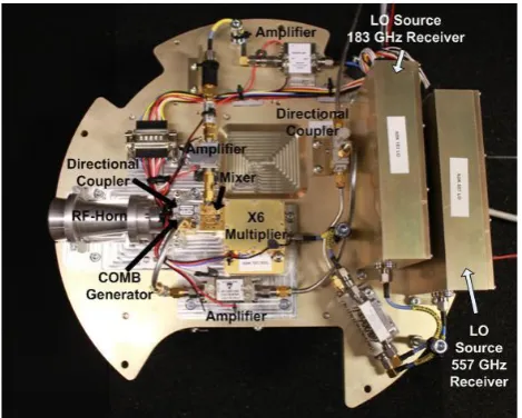
Figure 1. Pictures of the 557 GHz and the 183 GHz radiometers taken during the rocket assembly at Esrange, Kiruna, and their respective placement on the rocket. All lengths are in mm.

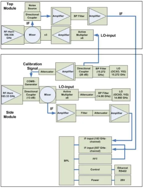
Figure 2. Layout of the top and side modules. The backend is located in the side module.

The observation period started at 40 km altitude for the 183 GHz radiometer and at nose cone ejection (approx. 60

km), for the 557 GHz radiometer. The observation period continues until approximately 100 s into the return trajectory.

During the observation time the instrument collected data with 300 Hz sampling rate for the 183 GHz receiver and 10

Hz for the 557 GHz receiver. For the 183 GHz radiometer, channel 183.310 GHz ±19.3 MHz was recorded from the

FFT backend data and in addition 182.264 GHz ±0.5 MHz, for the calibration signal. For the 557 GHz radiometer, the

channel 556.936 GHz ±19.3 MHz was recorded of the FFT backend data. The reason for limiting the spectral width is

to reduce the amount of data stored. Initially the data are stored locally in SDRAM, with limited capacity, and are

dumped to non-volatile data storage at the apogee, as well as after the return to an observation stop altitude. A further

step to reduce the amount of data is to vary the spectral bandwidth of the channels by keeping a high resolution, 67 kHz,

at the centre of the band and decrease the resolution by combining channels towards the band edges. By doing this, the

number of channels is reduced from 576 to 184. With lossless data compression using the variable resolution over the

spectrum, the recorded data set is reduced to approximately 12 MByte/100s observation. As mentioned above, the task

of building the backend, and housekeeping computing system for data handling was done by Omnisys Instruments AB.

2.2.

Measurement Accuracy and Calibration

A typical application for a radiometer in atmospheric or radio astronomical observation is to detect very weak

signals, buried in noise. If the system noise is completely uncorrelated, i.e. white noise, signal integration over

time will reduce the noise according to the radiometric equation (Rohlfs and Wilson 2000):

√

(1)

where

T

system

is the total system noise (

T

antenna

+

T

receiver ),

B

is the detection bandwidth,

τ

is the integration time,

and σ is the resulting standard deviation. In reality, the noise in a radiometer is a combination of white noise, the

DC (Direct Current) drift, and 1/f noise. The DC drift and 1/f noise limit the possibility of reducing the noise by

integration and an optimum integration time can be calculated by the Allan variance (Allan 1966). This means

that further integration will not improve the signal-to-noise ratio. Apart from the noise-originated instability of

the receiver, the gain of the receiver varies over time. This can, for instance, vary if the physical temperature of

the receiver changes and it implies that a calibration of the receiver is needed in order to be able to compensate

for the gain drift over the entire observation period. The time periods between calibration sequences should be

well within the characteristic time of the gain instability.

The most common calibration technique for radiometers is the use of a Dicke-switch (Dicke 1946), where the

reference signals are radiation from a black body at two different and specific, accurately known, temperatures,

PHot/PCold. The received power can be calculated according to Planck’s black body radiation law in the

Rayleigh-Fig. 1. Pictures of the 557 GHz and the 183 GHz radiometers taken

during the rocket assembly at Esrange, Kiruna, and their respective placement on the rocket. All lengths are in mm.

The observation period started at 40 km altitude for the 183 GHz radiometer and at nose cone ejection (ap-prox. 60 km) for the 557 GHz radiometer. The observation period continues until approximately 100 s into the return tra-jectory. During the observation time, the instrument collected data with 300 Hz sampling rate for the 183 GHz receiver and 10 Hz for the 557 GHz receiver. For the 183 GHz radiome-ter, channel 183.310 GHz±19.3 MHz was recorded from the FFT backend data and in addition 182.264 GHz±0.5 MHz, for the calibration signal. For the 557 GHz radiometer, the channel 556.936 GHz±19.3 MHz was recorded from the FFT backend data. The reason for limiting the spectral width is to reduce the amount of data stored. Initially, the data are stored locally in SDRAM, with limited capacity, and are dumped to non-volatile data storage at the apogee, as well as after the return to an observation stop altitude. A fur-ther step to reduce the amount of data is to vary the spec-tral bandwidth of the channels by keeping a high resolution, 67 kHz, at the centre of the band and decrease the resolu-tion by combining channels towards the band edges. By do-ing this, the number of channels is reduced from 576 to 184. With lossless data compression using the variable resolution

Figure 1. Pictures of the 557 GHz and the 183 GHz radiometers taken during the rocket assembly at Esrange, Kiruna, and their respective placement on the rocket. All lengths are in mm.

Figure 2. Layout of the top and side modules. The backend is located in the side module.

The observation period started at 40 km altitude for the 183 GHz radiometer and at nose cone ejection (approx. 60

km), for the 557 GHz radiometer. The observation period continues until approximately 100 s into the return trajectory.

During the observation time the instrument collected data with 300 Hz sampling rate for the 183 GHz receiver and 10

Hz for the 557 GHz receiver. For the 183 GHz radiometer, channel 183.310 GHz ±19.3 MHz was recorded from the

FFT backend data and in addition 182.264 GHz ±0.5 MHz, for the calibration signal. For the 557 GHz radiometer, the

channel 556.936 GHz ±19.3 MHz was recorded of the FFT backend data. The reason for limiting the spectral width is

to reduce the amount of data stored. Initially the data are stored locally in SDRAM, with limited capacity, and are

dumped to non-volatile data storage at the apogee, as well as after the return to an observation stop altitude. A further

step to reduce the amount of data is to vary the spectral bandwidth of the channels by keeping a high resolution, 67 kHz,

at the centre of the band and decrease the resolution by combining channels towards the band edges. By doing this, the

number of channels is reduced from 576 to 184. With lossless data compression using the variable resolution over the

spectrum, the recorded data set is reduced to approximately 12 MByte/100s observation. As mentioned above, the task

of building the backend, and housekeeping computing system for data handling was done by Omnisys Instruments AB.

2.2.

Measurement Accuracy and Calibration

A typical application for a radiometer in atmospheric or radio astronomical observation is to detect very weak

signals, buried in noise. If the system noise is completely uncorrelated, i.e. white noise, signal integration over

time will reduce the noise according to the radiometric equation (Rohlfs and Wilson 2000):

√

(1)

where

T

system

is the total system noise (

T

antenna

+

T

receiver

),

B

is the detection bandwidth,

τ

is the integration time,

and σ is the resulting standard deviation. In reality, the noise in a radiometer is a combination of white noise, the

DC (Direct Current) drift, and 1/f noise. The DC drift and 1/f noise limit the possibility of reducing the noise by

integration and an optimum integration time can be calculated by the Allan variance (Allan 1966). This means

that further integration will not improve the signal-to-noise ratio. Apart from the noise-originated instability of

the receiver, the gain of the receiver varies over time. This can, for instance, vary if the physical temperature of

the receiver changes and it implies that a calibration of the receiver is needed in order to be able to compensate

for the gain drift over the entire observation period. The time periods between calibration sequences should be

well within the characteristic time of the gain instability.

The most common calibration technique for radiometers is the use of a Dicke-switch (Dicke 1946), where the

reference signals are radiation from a black body at two different and specific, accurately known, temperatures,

P

Hot

/P

Cold

. The received power can be calculated according to Planck’s black body radiation law in the

Rayleigh-Fig. 2. Layout of the top and side modules. The backend is located

in the side module.

over the spectrum, the recorded data set is reduced to approx-imately 0.12 MByte s−1 observation. As mentioned above, the tasks of building the backend and housekeeping the com-puting system for data handling were done by Omnisys In-struments AB.

2.2 Measurement accuracy and calibration

A typical application for a radiometer in atmospheric or ra-dio astronomical observation is to detect very weak signals, buried in noise. If the system noise is completely uncorlated, i.e. white noise, signal integration over time will re-duce the noise according to the radiometric equation (Rohlfs and Wilson, 2000):

σ=T√System

Bτ (1)

whereTsystemis the total system noise (Tantenna+Treceiver),B is the detection bandwidth,τ is the integration time, andσ

is the resulting standard deviation. In reality, the noise in a radiometer is a combination of white noise, the DC (Direct Current) drift, and 1/f noise. The DC drift and 1/f noise limit the possibility of reducing the noise by integration, and an optimum integration time can be calculated by the Allan vari-ance (Allan, 1966). This means that further integration will

(4)

1362 O. Nystr¨om et al.: PHOCUS radiometer

Jeans limit (Rohlfs and Wilson 2000), and, assuming a perfectly matched single-mode waveguide, the received

power can be calculated as

(2)

where

k

B is the Boltzmann’s constant,

B

is the detection bandwidth, and

T

is the brightness temperature of the

black body. The receiver noise temperature is then calculated according to a well-known relation

(3)

where Y is the ratio P

Hot

/P

Cold

, i.e. the IF output power of the radiometer when exposed to the different loads.

This technique calibrates the entire receiver chain (optics, mixer, and Low Noise Amplifiers (LNAs)) and is

usually implemented by employing a opto-mechanical switch, e.g

.

, a chopper wheel or a mechanical switch

placed in the receiver input beam. Another common problem of the standard Dicke-switch calibration technique

is that no measurements can be performed during the calibration cycle, hence precious observation time has to

be sacrificed.

However, due to a very harsh environment on board of the rocket, in terms of acceleration, shock, and

vibration, as well as space constraints and extremely short observing time, a calibration system without any

moving parts, a fully electronic calibration system, is the only option for PHOCUS. For example, a signal from

a broadband calibrated noise source, instead of the hot load, could be injected through a directional coupler

between the Radio Frequency horn (RF-horn) and the mixer as in (Rose, Czekala et al. 2009), but unfortunately

at 183 GHz and 557 GHz such noise sources are not commercially available.

2.3.

The 183 GHz RF channel calibration system

The driver for the 183 GHz calibration system on the PHOCUS rocket was to consider the above mentioned

criteria, e.g. no moving parts and the space constraints. To achieve this, a calibration system with a stable pilot

signal injected through a directional coupler (Meyer and Kruger 1998) (-13dB coupling) between the RF-horn

antenna and the mixer was introduced. The pilot signal is placed 40 MHz away from the 183.31 GHz water

absorption line, the target for the observation, and thus allows continuous calibration without any loss of

observation time. With this calibration technique it is assumed that all receiver back-end channels experience

the same gain variations over the observation time. The pilot signal is generated from the LO source for the 557

GHz radiometer, which has a base frequency of 15.727 GHz. The reference signal is extracted from the LO

through a 20 dB directional coupler, amplified and fed to a harmonic mixer generating the pilot signal at

183.264 GHz (12

th

harmonic). The block diagram and layout of the radiometer with its calibration system can be

seen in Figure 3. The amplifier operates in saturation in order to keep the amplitude of the generated output

calibration signal insensitive to small fluctuations in the reference signal supplied.

Figure 3.Picture of the 183 GHz side module containing the radiometer, calibration system, and LOs for the 183 GHz and 557 GHz receivers. The backend is located on the back side of the radiometer base plate.

Right before the launch, the receiver noise temperature is measured by standard Y-factor technique in order to

obtain an absolute temperature reference. This is done by placing a hot (ambient temperature) and cold (LN2)

loads outside the rocket, at the radiometer signal window. During this calibration, the level of the pilot signal

Fig. 3. Picture of the 183 GHz side module containing the

radiome-ter, calibration system, and LOs for the 183 GHz and 557 GHz re-ceivers. The backend is located on the back side of the radiometer base plate.

not improve the signal-to-noise ratio. Apart from the noise-originated instability of the receiver, the gain of the receiver varies over time. This can, for instance, vary if the physi-cal temperature of the receiver changes, and it implies that a calibration of the receiver is needed in order to be able to compensate for the gain drift over the entire observation pe-riod. The time periods between calibration sequences should be well within the characteristic time of the gain instability.

The most common calibration technique for radiometers is the use of a Dicke-switch (Dicke, 1946), where the reference signals are radiation from a black body at two different and specific, accurately known, temperatures,PHot/PCold. The re-ceived power can be calculated according to Planck’s black body radiation law in the Rayleigh-Jeans limit (Rohlfs and Wilson, 2000), and, assuming a perfectly matched single-mode waveguide, the received power can be calculated as

P =kBBT (2)

where kB is the Boltzmann’s constant, B is the detection bandwidth, andT is the brightness temperature of the black body. The receiver noise temperature is then calculated ac-cording to a well-known relation:

Te=

THot−Y·TCold

Y−1 (3)

whereY is the ratioPHot/PCold, i.e. the IF output power of the radiometer when exposed to the different loads. This tech-nique calibrates the entire receiver chain (optics, mixer, and low-noise amplifiers, LNAs) and is usually implemented by employing a opto-mechanical switch (e.g. a chopper wheel or

referenced to the noise floor (ratio should be the same for hot- and cold loads) is recorded. During the flight, any drift of the gain in the receiver chain will result in a change in the pilot signal level relative to the baseline noise level.

2.4. The 557 GHz IF Channel Calibration System

The 557 GHz radiometer calibration utilizes a different technique. This calibration system is also fully electronic, for the same reasons as pointed out in the previous section. The much higher frequency makes it more difficult and expensive to generate signals that could be used as a pilot signal while, most importantly, introducing a directional coupler with its associated loss in front of the mixer would substantially increase the system noise. Following these considerations, the 557 GHz radiometer calibration is done by injecting broadband noise from a calibrated noise source, (Wireless Telecom Group), through a directional coupler between the mixer output and the first IF Amplifier (LNA), Figure 4. This scheme limits calibration of the 557 GHz receiver channel to the gain to the IF and back-end parts, the parts probably mostly affected by changing the ambient temperature.

Figure 4. Picture of the 557 GHz radiometer with the horn, noise source, coupler, and LNAs. The mixer and LO-multiplier is located on the other back side.

Since any measurements during the calibration would not be feasible, in contrast to the calibration system for the 183.31 GHz radiometer, the calibration is performed before the rocket reaches the altitude where the measurements should start. A second calibration is performed at the trajectory apogee, and the third calibration sequence is done once the rocket has reached an altitude below the altitude of interest. The drift in the receiver gain is measured between the calibration periods by measuring the difference between the baseline (independent on the load temperature) and the level with the calibration noise source is switched on. A decrease in the receiver gain would result in a smaller difference between the on/off calibration signal cases.

2.5. Horn design

The specifications of the far-field distribution for the 183 GHz and the 557 GHz radiometers required the beam width Full Width Half Maximum (FWHM) < 5° with side lobe level < -20 dB. A typical optical design for such a narrow beam would be a combination of a horn and additional focusing elements, e.g. off-axis mirrors or a lens. However, as a consequence of a very limited space available inside the rocket, an optical layout with a single larger sized horn was chosen, since it provides the most compact alternative and reduces the complexity of placement and alignment of additional optical elements. A narrow beam requires large dimensions of the horn; consequently the challenge is to obtain a large aperture while minimizing the length of the horn. Because of relatively narrow RF band required (183±0.02 GHz and 557±0.02 GHz), we have chosen a smooth-wall conical horn. This type of horn is known to employ multi-mode field propagation inside the horn. In the literature, several horn types and horn profiles are presented in order to control the mode conversion and to reduce the length (Olver, et al. 1994), (Mahmoud 1983), (Watson, Rudge et al. 1980), (James 1984), (Potter 1963), and (Pickett, Hardy et al. 1984)). The profiled horn shows very good performance for moderately compact sizes and FWHM of the order of 10° or wider. However, as a narrower beam is required the side lobes tend to increase rapidly compared to a longer, linearly tapered, horn. Since the relative bandwidth of operation is less than 5 %, a linearly tapered Picket horn (Pickett, Hardy et al. 1984), with a flared step, was selected for the design. In (Kittara, Jiralucksanawong et al. 2007), the choice of a flared step is reported to be superior over the

Fig. 4. Picture of the 557 GHz radiometer with the horn, noise

source, coupler, and LNAs. The mixer and LO-multiplier are lo-cated on the other back side.

grooved step. The Pickett-Potter horn gives a moderately compact design with good performance over approximately 15% bandwidth and has the advantage over, for instance, the corrugated horn, of simpler geometry and hence quicker production time. If necessary, bandwidth up to 30% can be achieved by adding more subsections in the horn as reported in (Yassin 2007). In the Potter horn, higher order modes are excited in the horn throat region by either a step discontinuity or a flared section (see Figure 5). The idea behind the Potter horn is to excite, besides the dominant TE11 mode, the higher order TM11 mode. In the conventional Potter horn

design, the step discontinuity of the single-mode circular waveguide provides balanced transformation of approximately 16 % of the dominant TE11 mode into the TM11 mode. This technique is referred to as the

“dual-mode conical horn” and has the characteristic of side lobe suppression and symmetric beam profiles (Potter 1963). The original design, by P. D. Potter, has been further developed in order to create a more compact layout by removing the phasing section of the horn and use instead the length of the flared section to obtain the appropriate relative phase between the modes (Pickett, Hardy et al. 1984).

In the horn design, presented here, the modal matching technique is used (Olver, et al. 1994). This algorithm provides calculation of the modal conversion throughout the horn and the resulting modal content at the horn aperture. As pointed out in (Kittara, Jiralucksanawong et al. 2007), other higher order modes apart from the TM11 mode will exist in the horn and excitation of, e.g., the TE12 mode at specific relative amplitude and phase

at the horn aperture could help improve the bandwidth performance. In the present horn design, we try to employ, besides the TE11, TM11, and TE12 mode, other higher order modes. For this purpose a mode matching

software was used in conjunction with a Matlab (Matlab 2011) optimization routine, which finds the optimum mode content at the aperture for the desired far-field distribution. The optimization function uses a modified version of the built in optimization routine with bound constraints on the variables, fminsearchbnd (D’Errico 2005). The function is based on the Nelder-Mead simplex search method (Lagarias and al. 1997).In the design, the goals are specified as i. desired beam width, ii. low side lobe levels and circularity, and iii. return loss below -30 dB. The optimization variables are shown in Figure 5, where h1 and α defines the step, and β and L the horn

conical section to obtain the desired modal phases at the horn aperture. The mode matching software used assumes that the discontinuity is excited only by modes of theTE1n and TM1n type, and due to symmetry of the

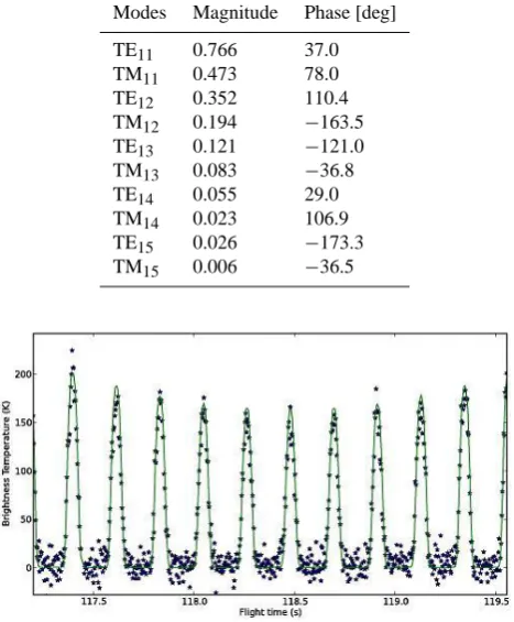
junction only modes of the TE1n and TM1n may be excited. In Table 2, the amplitude and phase of the first five

TE1n and TM1n are shown.

Figure 5. Horn profile of the horns with a flared step, defined by α and h1, generating higher order modes.

The final design was verified with Physical Optics (PO) software, MODAL, developed by NUIM (Gradziel 2011), which showed excellent agreement to the measured data, Figure 6.

The 183 GHz horn for SondRad was made out of aluminium alloy by machining with a computer controlled lathe. It was measured using Agilent PNA 8364B (Agilent Technologies Inc.) with frequency extension modules (OML Inc.). The far-field pattern of the horn was calculated via a Fourier transform of the near-filed scan and is shown in Figure 7 and Figure 8 with a FWHM of 4.7° and side lobe levels less than -40 dB.

Fig. 5. Horn profile of the horns with a flared step, defined byαand h1, generating higher order modes.

a mechanical switch placed in the receiver input beam). An-other common problem of the standard Dicke-switch calibra-tion technique is that no measurements can be performed dur-ing the calibration cycle; hence, precious observation time has to be sacrificed.

However, due to a very harsh environment on board of the rocket, in terms of acceleration, shock, and vibration, as well as space constraints and extremely short observing time, a calibration system without any moving parts, a fully elec-tronic calibration system, is the only option for PHOCUS. For example, a signal from a broadband calibrated noise source, instead of the hot load, could be injected through a directional coupler between the radio frequency horn (RF-horn) and the mixer as in Rose et al. (2009), but unfortu-nately at 183 GHz and 557 GHz such noise sources are not commercially available.

(5)

O. Nystr¨om et al.: PHOCUS radiometer 1363

Figure 6. Comparisons of Fourier transform of the near-filed scan data at 183.31 GHz to PO-simulations.

Figure 7. Measured far-field pattern of the horn at 183.31 GHz.

Figure 8. Contour plot of the far-field pattern of the measured horn at 183.31 GHz.

The 557 GHz horn is an exact scaled version of the 183 GHz horn but no measurements were performed because of the absence of suitable equipment at this frequency. The 557 GHz horn was produced by Radiometric Physics GmbH (Radiometric Physics Gmbh) by electroforming and the horn performance is expected to be the same as for the 183 GHz horn relying on exact scaling effect. Pictures of the two horns are presented in Figure 9.

Figure 9. Picture of the 183 GHz horn (top) and the 557 GHz horn (bottom). Fig. 6. Comparisons of Fourier transform of the near-filed scan data

at 183.31 GHz to PO-simulations.

loss of observation time. With this calibration technique, it is assumed that all receiver back-end channels experience the same gain variations over the observation time. The pi-lot signal is generated from the LO source for the 557 GHz radiometer, which has a base frequency of 15.727 GHz. The reference signal is extracted from the LO through a 20 dB directional coupler, amplified and fed into a harmonic mixer generating the pilot signal at 183.264 GHz (12th harmonic). The block diagram and layout of the radiometer with its cal-ibration system can be seen in Fig. 3. The amplifier operates in saturation in order to keep the amplitude of the generated output calibration signal insensitive to small fluctuations in the reference signal supplied.

Right before the launch, the receiver noise temperature is measured by standardY-factor technique in order to obtain an absolute temperature reference. This is done by placing hot (ambient temperature) and cold (LN2) loads outside the rocket, at the radiometer signal window. During this calibra-tion, the level of the pilot signal referenced to the noise floor (ratio should be the same for hot- and cold loads) is recorded. During the flight, any drift of the gain in the receiver chain will result in a change in the pilot signal level relative to the baseline noise level.

2.4 The 557 GHz IF channel calibration system

The 557 GHz radiometer calibration utilizes a different tech-nique. This calibration system is also fully electronic, for the same reasons as pointed out in the previous section. The much higher frequency makes it more difficult and expensive to generate signals that could be used as a pilot signal, while, most importantly, introducing a directional coupler with its associated loss in front of the mixer would substantially

Figure 6. Comparisons of Fourier transform of the near-filed scan data at 183.31 GHz to PO-simulations.

Figure 9. Picture of the 183 GHz horn (top) and the 557 GHz horn (bottom).

Fig. 7. Measured far-field pattern of the horn at 183.31 GHz.

increase the system noise. Following these considerations, the 557 GHz radiometer calibration is done by injecting broadband noise from a calibrated noise source, (Wireless Telecom Group, 2011), through a directional coupler be-tween the mixer output and the first IF amplifier (LNA) (Fig. 4). This scheme limits calibration of the 557 GHz re-ceiver channel to the gain to the IF and back-end parts, the parts probably mostly affected by changing the ambient temperature.

Since any measurements during the calibration would not be feasible, in contrast to the calibration system for the 183.31 GHz radiometer, the calibration is performed be-fore the rocket reaches the altitude where the measurements should start. A second calibration is performed at the trajec-tory apogee, and the third calibration sequence is done once the rocket has reached an altitude below the altitude of in-terest. The drift in the receiver gain is measured between the calibration periods by measuring the difference between the baseline (independent on the load temperature) and the level with the calibration noise source switched on. A decrease in the receiver gain would result in a smaller difference between the on/off calibration signal cases.

2.5 Horn design

The specifications of the far-field distribution for the 183 GHz and the 557 GHz radiometers required the beam width full width half maximum (FWHM)<5◦with side-lobe level<−20 dB. A typical optical design for such a narrow beam would be a combination of a horn and additional fo-cusing elements, e.g. off-axis mirrors or a lens. However, as a consequence of a very limited space available inside the rocket, an optical layout with a single larger sized horn was chosen, since it provides the most compact alternative and

(6)

1364 O. Nystr¨om et al.: PHOCUS radiometer

The 557 GHz horn is an exact scaled version of the 183 GHz horn but no measurements were performed

because of the absence of suitable equipment at this frequency. The 557 GHz horn was produced by

Radiometric Physics GmbH (Radiometric Physics Gmbh) by electroforming and the horn performance is

expected to be the same as for the 183 GHz horn relying on exact scaling effect. Pictures of the two horns are

presented in Figure 9.

Figure 9. Picture of the 183 GHz horn (top) and the 557 GHz horn (bottom).

Fig. 8. Contour plot of the far-field pattern of the measured horn at

183.31 GHz.

reduces the complexity of placement and alignment of addi-tional optical elements. A narrow beam requires large dimen-sions of the horn; consequently, the challenge is to obtain a large aperture while minimizing the length of the horn. Be-cause of relatively narrow RF band required (183±0.02 GHz and 557±0.02 GHz), we have chosen a smooth-wall coni-cal horn. This type of horn is known to employ multi-mode field propagation inside the horn. In the literature, several horn types and horn profiles are presented in order to con-trol the mode conversion and to reduce the length (Olver et al., 1994; Mahmoud, 1983; Watson et al., 1980; James, 1984; Potter, 1963; Pickett et al., 1984). The profiled horn shows very good performance for moderately compact sizes and FWHM of the order of 10◦or wider. However, as a narrower beam is required, the side lobes tend to increase rapidly com-pared to a longer, linearly tapered, horn. Since the relative bandwidth of operation is less than 5 %, a linearly tapered Picket horn (Pickett et al., 1984), with a flared step, was se-lected for the design. In Kittara et al. (2007), the choice of a flared step is reported to be superior over the grooved step. The Pickett-Potter horn gives a moderately compact design with good performance over approximately 15 % bandwidth and has the advantage over, for instance, the corrugated horn of simpler geometry and hence quicker production time. If necessary, bandwidth up to 30 % can be achieved by adding more subsections in the horn, as reported in Yassin (2007). In the Potter horn, higher order modes are excited in the horn throat region by either a step discontinuity or a flared section (see Fig. 5). The idea behind the Potter horn is to excite, be-sides the dominant TE11mode, the higher order TM11mode.

Figure 7. Measured far-field pattern of the horn at 183.31 GHz.

Figure 9. Picture of the 183 GHz horn (top) and the 557 GHz horn (bottom). _{Fig. 9. Picture of the 183 GHz horn (top) and the 557 GHz horn}

(bottom).

In the conventional Potter horn design, the step discontinu-ity of the single-mode circular waveguide provides balanced transformation of approximately 16 % of the dominant TE11 mode into the TM11 mode. This technique is referred to as the “dual-mode conical horn” and has the characteristic of side-lobe suppression and symmetric beam profiles (Potter, 1963). The original design, by P. D. Potter, has been further developed in order to create a more compact layout by re-moving the phasing section of the horn and use instead the length of the flared section to obtain the appropriate relative phase between the modes (Pickett et al., 1984).

(7)

O. Nystr¨om et al.: PHOCUS radiometer 1365

3.

Laboratory Measurements

3.1.

Laboratory Measurements of the 183 GHZ Calibration System

The receiver temperature and the pilot signal measurements performed in the laboratory are presented in

Figure 10 and Figure 11. The mean value and standard deviation are plotted together with the noise temperature,

where the mean is calculated for the central channels where the resolution is the highest, 67 kHz. At the band

edges, the channels are combined in order to reduce the data storage. The data in Figure 10 and Figure 11 are

integrated over 10 seconds and the calibration accuracy (repeatability) is estimated to less than 2 % and is

calculated as

( ) ( )

(4)

( )

(5)

Figure 10. Laboratory measurements of the 183 GHz receiver noise temperature.

Figure 11.Pilot signal with liquid nitrogen and room temperature

loads.

During the observation period the measurement rate is 300 Hz, resulting in an integration time of 3.3 ms per

spectrum. In order to determine if the required integration time for the observation is allowed by the actual

stability of the receiver, its output was measured and the Allan variance was calculated. Notice that the

integration time in order to obtain a stable pilot signal is independent of the integration time used for the

observation data, which might be shorter in order to dissect the mesosphere and obtain the desired altitude

profile. The observations will typically be in blocks of 0.1 s, i.e

.,

integration over 30 spectra. The Allan variance

of the 183 GHz radiometer is shown in Figure 12 for both the observation channels and the channel where the

pilot signal is located. Longer measurements are needed in order to find the integration limit, but the internal

memory in the backend has limited capacity and the measurements over time periods >150 seconds are not

possible due to the limited data storage capacity. During the flight, measurement time will be less than 100

seconds, where after the data is stored on an SD-card and an USB-memory, and the internal memory is cleared

and a new measurement session can take place.

Figure 12. Allan variance for the 183 GHz receiver (left) and the Allan variance for the receiver channel containing the pilot signal. Fig. 10. Laboratory measurements of the 183 GHz receiver noise

temperature.

modal phases at the horn aperture. The mode matching soft-ware used assumes that the discontinuity is excited only by modes of the TE1n and TM1n type, and, due to symmetry of the junction, only modes of the TE1n and TM1n may be excited. In Table 2, the amplitude and phase of the first five TE1nand TM1nare shown.

The final design was verified with physical optics (PO) software, MODAL, developed by NUIM (Gradziel, 2011), which showed excellent agreement to the measured data (Fig. 6).

The 183 GHz horn for SondRad was made out of alu-minium alloy by machining with a computer-controlled lathe. It was measured using Agilent PNA 8364B (Agilent Technologies Inc., 2011) with frequency extension modules (OML Inc., 2011). The far-field pattern of the horn was cal-culated via a Fourier transform of the near-filed scan and is shown in Figs. 7 and 8 with a FWHM of 4.7◦and side-lobe levels less than−40 dB.

The 557 GHz horn is an exact scaled version of the 183 GHz horn, but no measurements were performed be-cause of the absence of suitable equipment at this frequency. The 557 GHz horn was produced by Radiometric Physics GmbH (Radiometric Physics GmbH, 2011) by electroform-ing, and the horn performance is expected to be the same as for the 183 GHz horn relying on exact scaling effect. Pictures of the two horns are presented in Fig. 9.

3 Laboratory measurements

3.1 Laboratory measurements of the 183 GHz calibration system

The receiver temperature and the pilot signal measurements performed in the laboratory are presented in Figs. 10 and 11. The mean value and standard deviation are plotted to-gether with the noise temperature, where the mean is cal-culated for the central channels where the resolution is the highest, 67 kHz. At the band edges, the channels are com-bined in order to reduce the data storage. The data in Figs. 10

3.

Laboratory Measurements

3.1.

Laboratory Measurements of the 183 GHZ Calibration System

The receiver temperature and the pilot signal measurements performed in the laboratory are presented in

Figure 10 and Figure 11. The mean value and standard deviation are plotted together with the noise temperature,

where the mean is calculated for the central channels where the resolution is the highest, 67 kHz. At the band

edges, the channels are combined in order to reduce the data storage. The data in Figure 10 and Figure 11 are

integrated over 10 seconds and the calibration accuracy (repeatability) is estimated to less than 2 % and is

calculated as

( ) ( )

(4)

( )

(5)

Figure 10. Laboratory measurements of the 183 GHz receiver noise temperature.

loads.

During the observation period the measurement rate is 300 Hz, resulting in an integration time of 3.3 ms per

spectrum. In order to determine if the required integration time for the observation is allowed by the actual

stability of the receiver, its output was measured and the Allan variance was calculated. Notice that the

integration time in order to obtain a stable pilot signal is independent of the integration time used for the

observation data, which might be shorter in order to dissect the mesosphere and obtain the desired altitude

profile. The observations will typically be in blocks of 0.1 s, i.e

.,

integration over 30 spectra. The Allan variance

of the 183 GHz radiometer is shown in Figure 12 for both the observation channels and the channel where the

pilot signal is located. Longer measurements are needed in order to find the integration limit, but the internal

memory in the backend has limited capacity and the measurements over time periods >150 seconds are not

possible due to the limited data storage capacity. During the flight, measurement time will be less than 100

seconds, where after the data is stored on an SD-card and an USB-memory, and the internal memory is cleared

and a new measurement session can take place.

Figure 12. Allan variance for the 183 GHz receiver (left) and the Allan variance for the receiver channel containing the pilot signal. Fig. 11. Pilot signal with liquid nitrogen and room temperature

loads.

and 11 are integrated over 10 s, and the calibration accuracy (repeatability) is estimated to be less than 2 % and is calcu-lated as

1=(Peak Hot−Baseline Hot)

−(Peak Cold−Baseline Cold) (4)

Uncertainty(%)= 1

Peak−Baseline×100 (5)

During the observation period, the measurement rate is 300 Hz, resulting in an integration time of 3.3 ms per spec-trum. In order to determine if the required integration time for the observation is allowed by the actual stability of the receiver, its output was measured and the Allan variance was calculated. Notice that the integration time in order to ob-tain a stable pilot signal is independent of the integration time used for the observation data, which might be shorter in order to dissect the mesosphere and obtain the desired al-titude profile. The observations will typically be in blocks of 0.1 s, i.e. integration over 30 spectra. The Allan variance of the 183 GHz radiometer is shown in Fig. 12 for both the observation channels and the channel where the pilot signal is located. Longer measurements are needed in order to find the integration limit, but the internal memory in the backend has limited capacity, and the measurements over time periods

>150 s are not possible due to the limited data storage ca-pacity. During the flight, measurement time will be less than 100 s, and after the data are stored on an SD-card and USB-memory and the internal USB-memory is cleared, a new measure-ment session can take place.

3.2 Laboratory measurements of the 557 GHz calibration system

The stability for the 557 GHz receiver was measured by sam-pling the output signal, and the Allan variance time was cal-culated in order to obtain the optimum integration time. Fig-ure 13 shows the Allan variance plots for the receiver without and with the calibration noise source switched on.

(8)

1366 O. Nystr¨om et al.: PHOCUS radiometer 3. Laboratory Measurements

3.1. Laboratory Measurements of the 183 GHZ Calibration System

The receiver temperature and the pilot signal measurements performed in the laboratory are presented in Figure 10 and Figure 11. The mean value and standard deviation are plotted together with the noise temperature, where the mean is calculated for the central channels where the resolution is the highest, 67 kHz. At the band edges, the channels are combined in order to reduce the data storage. The data in Figure 10 and Figure 11 are integrated over 10 seconds and the calibration accuracy (repeatability) is estimated to less than 2 % and is calculated as

( ) ( ) (4)

( )

(5)

Figure 10. Laboratory measurements of the 183 GHz receiver noise temperature.

loads.

During the observation period the measurement rate is 300 Hz, resulting in an integration time of 3.3 ms per spectrum. In order to determine if the required integration time for the observation is allowed by the actual stability of the receiver, its output was measured and the Allan variance was calculated. Notice that the integration time in order to obtain a stable pilot signal is independent of the integration time used for the observation data, which might be shorter in order to dissect the mesosphere and obtain the desired altitude profile. The observations will typically be in blocks of 0.1 s, i.e., integration over 30 spectra. The Allan variance of the 183 GHz radiometer is shown in Figure 12 for both the observation channels and the channel where the pilot signal is located. Longer measurements are needed in order to find the integration limit, but the internal memory in the backend has limited capacity and the measurements over time periods >150 seconds are not possible due to the limited data storage capacity. During the flight, measurement time will be less than 100 seconds, where after the data is stored on an SD-card and an USB-memory, and the internal memory is cleared and a new measurement session can take place.

Figure 12. Allan variance for the 183 GHz receiver (left) and the Allan variance for the receiver channel containing the pilot signal.

Fig. 12. Allan variance for the 183 GHz receiver (left) and the Allan variance for the receiver channel containing the pilot signal.

3.2. Laboratory Measurements of the 557 GHZ Calibration System

The stability for the 557 GHz receiver was measured by sampling the output signal and the Allan variance time was calculated in order to obtain the optimum integration time. Figure 13 shows the Allan variance plots for the receiver without and with the calibration noise source switched on.

Figure 13. Allan variance plots (77K load) with the noise source off (left) and the noise source on (right).

It can be seen in Figure 13 that the Allan variance plot agrees very well with the radiometric equation, (1), i.e.,

the white noise component prevail over 1/f noise for the represented time scale. The total flight period, one way, of approximately 60-100 seconds (nose cone ejection - apogee) is well within the measured Allan variance. During flight, calibration with an integration time of approximately 5 seconds was used for this radiometer, which is well within the feasible integration time with the source on.

Figure 14. Laboratory measurements of the receiver temperature with fan cooling (left) and without cooling (right).

The receiver temperature is also dependent on the physical temperature surrounding the instrument; hence the receiver temperature might differ from the laboratory measurements, where a fan was used for cooling. Figure 14 shows two different laboratory measurements, with and without fan cooling (fan directed towards the back end). It can be seen that the receiver noise temperature has increased by 179.9 K (mean value) when the receiver physical temperature is increased by 2.4 °C for the 557GHz frontend and 15.7 °C for the back end. The mean value, standard deviation, and uncertainty of the factor measurement are plotted. The uncertainty in the Y-factor measurement is estimated by the use of the radiometer equation. With a system temperature of 4200 K, a bandwidth of 67 kHz, and the integration time of 10 seconds, this gives a standard deviation of 5.13K. This accuracy leads to an uncertainty in the cold measurement of 6.41% and 1.71% at 300K. A total uncertainty in the Y-factor of 8.1% results in an uncertainty of 340.5K in the receiver noise temperature.

Figure 15 shows the measured temperature for 80K and 300K, and with the noise signal switched on. This figure illustrates well the concept of the calibration method where the difference in level between the baseline with and without the noise source should be the same independent on the antenna temperature. If the system gain varies, this difference will vary as well, i.e., a drop in the system gain would result in a decrease in the difference of the levels (source on/off).

Fig. 13. Allan variance plots (77 K load) with the noise source off (left) and the noise source on (right).

It can be seen in Fig. 13 that the Allan variance plot agrees very well with the radiometric equation, Eq. (1), i.e. the white noise component prevails over 1/f noise for the represented time scale. The total flight period (one way) of approximately 60–100 s (nose cone ejection – apogee) is well within the measured Allan variance. During flight, calibration with an integration time of approximately 5 s was used for this ra-diometer, which is well within the feasible integration time with the source on.

The receiver temperature is also dependent on the phys-ical temperature surrounding the instrument; hence the re-ceiver temperature might differ from the laboratory measure-ments, where a fan was used for cooling. Figure 14 shows two different laboratory measurements, with and without fan cooling (fan directed towards the back end). It can be seen that the receiver noise temperature has increased by 179.9 K (mean value) when the receiver physical temperature is in-creased by 2.4◦C for the 557 GHz front end and 15.7◦C for the back end. The mean value, standard deviation, and un-certainty of theY-factor measurement are plotted. The un-certainty in the Y-factor measurement is estimated by the use of the radiometer equation. With a system temperature of 4200 K, a bandwidth of 67 kHz, and the integration time of 10 seconds, this gives a standard deviation of 5.13 K. This accuracy leads to an uncertainty in the cold measurement of 6.41 % and 1.71 % at 300 K. A total uncertainty in the Y -factor of 8.1 % results in an uncertainty of 340.5 K in the receiver noise temperature.

Figure 15 shows the measured temperature for 80K and 300 K, and with the noise signal switched on. This figure il-lustrates well the concept of the calibration method, where the difference in level between the baseline with and without the noise source should be the same independent on the an-tenna temperature. If the system gain varies, this difference will vary as well, i.e. a drop in the system gain would result in a decrease in the difference of the levels (source on/off).

In Fig. 16, the calibration error, i.e. the uncertainty of the temperature levels relative to the baseline, is plotted for the two measurements with different physical, stable, physical operating temperatures. This is the difference between the calibration level and the baseline level, as the load tempera-ture is changed from 80 K to 300 K calculated as

err=((300 K+Noise ON)−(300 Kload))

−((80 Kload+Noise ON)−(80 Kload)) , (6) and it can be seen that the standard deviations of the calibra-tion, over the central channels, are approximately the same in the two measurements: 11.3 K and 13.7 K (7 K over all channels).

(9)

O. Nystr¨om et al.: PHOCUS radiometer 1367 3.2. Laboratory Measurements of the 557 GHZ Calibration System

The stability for the 557 GHz receiver was measured by sampling the output signal and the Allan variance time was calculated in order to obtain the optimum integration time. Figure 13 shows the Allan variance plots for the receiver without and with the calibration noise source switched on.

Figure 13. Allan variance plots (77K load) with the noise source off (left) and the noise source on (right).

It can be seen in Figure 13 that the Allan variance plot agrees very well with the radiometric equation, (1), i.e.,

the white noise component prevail over 1/f noise for the represented time scale. The total flight period, one way, of approximately 60-100 seconds (nose cone ejection - apogee) is well within the measured Allan variance. During flight, calibration with an integration time of approximately 5 seconds was used for this radiometer, which is well within the feasible integration time with the source on.

Figure 14. Laboratory measurements of the receiver temperature with fan cooling (left) and without cooling (right).

The receiver temperature is also dependent on the physical temperature surrounding the instrument; hence the receiver temperature might differ from the laboratory measurements, where a fan was used for cooling. Figure 14 shows two different laboratory measurements, with and without fan cooling (fan directed towards the back end). It can be seen that the receiver noise temperature has increased by 179.9 K (mean value) when the receiver physical temperature is increased by 2.4 °C for the 557GHz frontend and 15.7 °C for the back end. The mean value, standard deviation, and uncertainty of the factor measurement are plotted. The uncertainty in the Y-factor measurement is estimated by the use of the radiometer equation. With a system temperature of 4200 K, a bandwidth of 67 kHz, and the integration time of 10 seconds, this gives a standard deviation of 5.13K. This accuracy leads to an uncertainty in the cold measurement of 6.41% and 1.71% at 300K. A total uncertainty in the Y-factor of 8.1% results in an uncertainty of 340.5K in the receiver noise temperature.

Figure 15 shows the measured temperature for 80K and 300K, and with the noise signal switched on. This figure illustrates well the concept of the calibration method where the difference in level between the baseline with and without the noise source should be the same independent on the antenna temperature. If the system gain varies, this difference will vary as well, i.e., a drop in the system gain would result in a decrease in the difference of the levels (source on/off).

Fig. 14. Laboratory measurements of the receiver temperature with fan cooling (left) and without cooling (right).

Figure 15. Measured temperature (in the load coordinate system) for 80K and 300K and with the noise signal switched on.

In Figure 16, the calibration error, i.e., the uncertainty of the temperature levels relative to the baseline is plotted for the two measurements with different physical, and stable, physical operating temperatures. This is the difference between the calibration level and the baseline level as the load temperature is changed from 80K to 300K calculated as

(( ) ( ))

(( ) ( )) (6)

and it can be seen that the standard deviation of the calibration, over the central channels, are approximately the same in the two measurements, 11.3 K and 13.7 K (7 K over all channels).

Figure 16. Calibration uncertainty of the receiver calibration for two different physical tempertures of the receiver. The calibration uncertainty remains unaffected for a increase in receiver noise temperture of 136K. The central channels with 67 kHz bandwidth is considered in the calculations.

The standard deviation of 12 K can be compared to the fluctuations between channels in two consecutive measurements performed with an 80K load, Figure 17. The level of fluctuations between channels is less in this case, with a standard deviation 7.9 K (4.2 K over all channels) compared to 12 K (7 K) with the noise source. The higher fluctuation in the calibration is expected since the system noise temperature (Treceiver+Tantenna) is

significantly higher (1300 K) with the noise source switched on. The standard deviation is slightly higher than calculated theoretical values based on the radiometric equation, resulting in a standard deviation of 5 K for the measurements of the 80K load (Tsystem=4100K) and 6.6 K for the measurements with the noise source switched

on (Tsystem=5400K). Prior to the rocket lift-off, a liquid cooling system is engaged and attached to the backend

base plate in order to avoid the temperature rising if the countdown is put on hold for a long time.

Fig. 15. Measured temperature (in the load coordinate system) for

80 K and 300 K and with the noise signal switched on.

with the noise source switched on. The standard deviation is slightly higher than calculated theoretical values based on the radiometric equation, resulting in a standard deviation of 5 K for the measurements of the 80 K load (Tsystem= 4100 K) and 6.6 K for the measurements with the noise source switched on (Tsystem= 5400 K). Prior to the rocket lift-off, a liquid cooling system is engaged and attached to the backend base plate in order to avoid the temperature rising, if the count-down is put on hold for a long time.

Absolute receiver noise temperature measurement prior to flight will not be possible due to the rocket nose cone place-ment, but the calibration procedure for gain variations is in-dependent on the physical temperature of the instrument and the antenna load; hence, a reference for the gain variations is obtained by switching on/off the calibrated noise source. In Fig. 18, the calculated receiver noise temperature for the two measurements with different physical temperatures of the re-ceiver is plotted. Included in the plot is also the corrected curve of measurement no. 2, i.e. the measurement at a higher physical temperature calibrated with respect to measurement no. 1. The calibration procedure is performed by calculation of the ratios of the radiometer counts between the antenna signal and with the calibrated noise source switched on for both measurements:

11=

Calibration 1 (Counts (Load))

Calibration 1 (Counts (Load + Noise Source)) (7)

12=

Calibration 2 (Counts (Load))

Calibration 2 (Counts (Load + Noise Source)) (8) TheY-factor is then corrected by the difference in the ra-tios as

Yfactor corrected=Yfactor+(11−12). (9) The residual difference after calibrating the spectra is

<50 K, which results in a calibration uncertainty<1.25 %, assuming 4000 K receiver noise temperature.

4 Discussion on flight results and post-flight calibration

The laboratory results presented in the previous sections were performed at temperatures in the range 25–35◦_{C. At}

each measurement session, the physical temperature of the instrument was stable (<±0.05◦_{C). The calibration system}

was designed based on the assumption that the instrument temperature would be reasonably stable during the short ob-servation period, for which laboratory measurements of the calibration system have indicated reliable performance. Fig-ures 19 and 20 show laboratory measurements of the radio-metric counts and temperature over 100 s together with a lin-ear fit of the data. The temperature and the pilot signal ampli-tude remain constant with self-heating of the instrument and an engaged table fan for temperature stabilization.

However, we observed that the instrument temperature increased significantly after the launch, with the tempera-ture changing from 16 to 28◦C over the observation period. That makes the assumption of stable physical temperature obviously not valid. The extreme increase in the tempera-ture, 12◦_{C over less than 4 min (!), was not expected, since}

the same increase in temperature during laboratory measure-ments takes almost 1.5 h. The exact cause of the temperature rise is not clear, but the major difference between laboratory measurements and the flight sequence is the lack of cooling through convection at high altitudes. A rise in temperature of the rocket structure was expected but should not exceed 70– 80◦C, and there are only a few attachment points between

(10)

1368 O. Nystr¨om et al.: PHOCUS radiometer

Figure 15. Measured temperature (in the load coordinate system) for 80K and 300K and with the noise signal switched on.

In Figure 16, the calibration error, i.e., the uncertainty of the temperature levels relative to the baseline is plotted for the two measurements with different physical, and stable, physical operating temperatures. This is the difference between the calibration level and the baseline level as the load temperature is changed from 80K to 300K calculated as

(( ) ( ))

(( ) ( )) (6)

and it can be seen that the standard deviation of the calibration, over the central channels, are approximately the same in the two measurements, 11.3 K and 13.7 K (7 K over all channels).

Figure 16. Calibration uncertainty of the receiver calibration for two different physical tempertures of the receiver. The calibration uncertainty remains unaffected for a increase in receiver noise temperture of 136K. The central channels with 67 kHz bandwidth is considered in the calculations.

The standard deviation of 12 K can be compared to the fluctuations between channels in two consecutive measurements performed with an 80K load, Figure 17. The level of fluctuations between channels is less in this case, with a standard deviation 7.9 K (4.2 K over all channels) compared to 12 K (7 K) with the noise source. The higher fluctuation in the calibration is expected since the system noise temperature (Treceiver+Tantenna) is significantly higher (1300 K) with the noise source switched on. The standard deviation is slightly higher than calculated theoretical values based on the radiometric equation, resulting in a standard deviation of 5 K for the measurements of the 80K load (Tsystem=4100K) and 6.6 K for the measurements with the noise source switched on (Tsystem=5400K). Prior to the rocket lift-off, a liquid cooling system is engaged and attached to the backend base plate in order to avoid the temperature rising if the countdown is put on hold for a long time.

Fig. 16. Calibration uncertainty of the receiver calibration for two different physical temperature of the receiver. The calibration uncertainty

remains unaffected for a increase in receiver noise temperature of 136 K. The central channels with 67 kHz bandwidth is considered in the calculations.

Figure 17. To consecutive 10 seconds measurements performed with a load temperature of 77K. The standard deviation over the central channels is 7.9 K, compared to 12 K with the noise source switched on.

Absolute receiver noise temperature measurement prior to flight will not be possible due to the rocket nose

cone placement, but the calibration procedure for gain variations is independent on the physical temperature of

the instrument and the antenna load, hence a reference for the gain variations is obtained by switching on/off the

calibrated noise source. In Figure

18

, the calculated receiver noise temperature for the two measurements with

different physical temperatures of the receiver is plotted. Included in the plot is also the corrected curve of

measurement nr 2, i.e

.,

the measurement at a higher physical temperature calibrated with respect to

measurement nr 1. The calibration procedure is performed by calculation of the ratios of the radiometer counts

between the antenna signal and with the calibrated noise source switched on for both measurements

( ( ))

(7)

( ( ))

(8)

The Y-factor is then corrected by the difference in the ratios as

(

)

(9)

The residual difference after calibrating the spectra is < 50 K which results in a calibration uncertainty < 1.25 %,

assuming 4000 K receiver noise temperature.

Figure 18. Measured receiver noise temperature for two measurements with different physical temperatures of the receiver and the calibrated curve. The calibrated curve shows a residual offset of 46.23 K which indicates a calibration error of 1.16%.

4.

Discussion on Flight Results and Post-Flight Calibration

The laboratory results presented in the previous sections were performed at temperatures in the range

25-Fig. 17. Two consecutive 10 s measurements performed with a load

temperature of 77 K: the standard deviation over the central chan-nels is 7.9 K, compared to 12 K with the noise source switched on.

Figure 17. To consecutive 10 seconds measurements performed with a load temperature of 77K. The standard deviation over the central channels is 7.9 K, compared to 12 K with the noise source switched on.

Absolute receiver noise temperature measurement prior to flight will not be possible due to the rocket nose

cone placement, but the calibration procedure for gain variations is independent on the physical temperature of

the instrument and the antenna load, hence a reference for the gain variations is obtained by switching on/off the

calibrated noise source. In Figure

18

, the calculated receiver noise temperature for the two measurements with

different physical temperatures of the receiver is plotted. Included in the plot is also the corrected curve of

measurement nr 2, i.e

.,

the measurement at a higher physical temperature calibrated with respect to

measurement nr 1. The calibration procedure is performed by calculat