International Journal of Industrial Engineering Computations 6 (2015) 457–468
Contents lists available at GrowingScience
International Journal of Industrial Engineering Computations
homepage: www.GrowingScience.com/ijiec
A Markov chain analysis of the effectiveness of drum-buffer-rope material flow
management in job shop environment
Masoud Rabbani* and Fahimeh Tanhaie
School of Industrial Engineering, College of Engineering, University of Tehran, Tehran, Iran
C H R O N I C L E A B S T R A C T
Article history: Received May 1 2015 Received in Revised Format May 10 2015
Accepted June 10 2015 Available online June 14 2015
The theory of constraints is an approach for production planning and control, which emphasizes on the constraints in the system to increase throughput. The theory of constraints is often referred to as Drum-Buffer-Rope developed originally by Goldratt. Drum-Buffer-Rope uses the drum or constraint to create a schedule based on the finite capacity of the first bottleneck. Because of complexity of the job shop environment, Drum-Buffer-Rope material flow management has very little attention to job shop environment. The objective of this paper is to apply the Drum-Buffer-Rope technique in the job shop environment using a Markov chain analysis to compare traditional method with Drum-Buffer-Rope. Four measurement parameters were considered and the result showed the advantage of Drum-Buffer-Rope approach compared with traditional one.
© 2015 Growing Science Ltd. All rights reserved
Keywords:
Theory of constraints Drum-Buffer-Rope Traditional method Markov chain
1. Introduction
The theory of constraints (TOC) is a management methodology developed by Goldratt in the mid-1980s (Goldratt & Fox, 1986). Every system must have at least one constraint and if this condition were not true, a real system could make unlimited profit. So a constraint is anything that prevents a system from achieving higher performance (Goldratt, 1988). The existence of constraints represents opportunities for improvement. Because constraints determine the performance of a system, a slow elevation of the system’s constraints will improve its performance so TOC views constraints as positive. In the early 1990s, Goldratt (1990) improved TOC by an effective management philosophy on improvement based on identifying the constraints to increase throughput. TOC’s approach is based on a five step process:
Identify the system constraint(s) Exploit the constraint(s)
Subordinate all other decision Elevate the constraint
Do not let inertia become the system constraint
The TOC is often referred to as Drum-Buffer-Rope (DBR) developed originally by Goldratt in the 1980s (Goldratt & Fox, 1986). DBR uses the protective capacity to eliminate the time delays to guarantee the bottleneck resource stays on schedule and customer orders are shipped on time (Chakravorty & Atwater, 2005). DBR uses the drum or constraint to create a schedule based on the finite capacity of the first bottleneck, buffer which protects the drum scheduling from variation. The rope is a communication device that connects the capacity constrained resource (CCR) to the material release point and controls the arrival of raw material to the production system (Schragenheim & Ronen, 1990). Rope generates the timely release of just the right materials into the system at just the right time (Wu et al., 1994).
This paper is begun with a description of DBR scheduling logic and a literature review that has related to this study is discussed in section 2. Then proposed approach is explained in section 3 .In section 4 and 5 a Markov chain analysis is applied to compare traditional method with Drum-Buffer-Rope. Finally, the conclusions and future development are showed in section 6.
2. Literature review
TOC normally has two major components. First, it focuses on the five steps of on-going improvement, the DBR scheduling, and the buffer management information system. The second component of TOC is an approach for solving complex problems called the thinking process (Rahman, 1998). Ray et al. (2008) proposed an integrated model by combining Laplace criterion and TOC into a single evaluation model in a multiproduct constraint resource environment. Pegels and Watrous (2005) applied the TOC to a bottleneck operation in a manufacturing plant and eliminated the constraint that prevented productivity at the plant. Bozzone (2002) introduced the theory of delays and claimed that this name is better than TOC because all constraints create delays but not all delays are caused by constraints. Rand (2000) explored the relationship between the ideas developed in the third novel, critical chain, by Goldratt (Goldratt, 1997) and the PERT/CPM approach. He showed the application of the theory of constraints on how management deal with human behaviour in constructing and managing the project network.
Many of papers compared the TOC flow management with material requirement planning (MRP) and just in time (JIT). For example Gupta and Snyder (2009) compared TOC (i) with MRP, (ii) with JIT, and (iii) with both MRP and JIT together and concluded that TOC compete effectively against MRP and JIT. Sale and Inman (2003) compared the performance of companies under TOC and JIT approach. They indicated that the greatest performance and improvement accrued under TOC approach. Choragi et al. (2008) compared seven different production control systems in a flow shop environment. The result showed that no single production control system was best under all conditions and it depended not only on the type of manufacturing strategy but also on the values of the input parameters.
protective capacity and production times. In DBR, any job that is not processed at the system’s first bottleneck is referred as a free good. Since free goods are not processed at the system’s first bottleneck, very little attention has been given to these jobs in DBR (Chakravorty & Verhoeven, 1996). Chakravorty and Atwater (2005) found that the performance of DBR is very sensitive to changes in the level of free goods release into the operation and claimed that schedulers of job shop environment using DBR need to be known of how orders of these items are scheduled.
Schragenheim and Dettmer (2000) introduced simplified drum buffer rope (S-DBR). SDBR is based on the same concept as traditional DBR. The only different is that in S_DBR the market demand is the major system constraint. Lee et al. (2010) examined two conditions that handled with SDBR solutions. They considered following characteristics and solved an example: (1) capacity constraint resource (CCR) is not always located in the middle of the routing. (2) Multiple CCRs can exist rather than the assumption of just one CCR. Chang and Huang (2013) provided a simple effective way to determine due dates and release dates of orders and jobs. They claimed that managers could easily use the proposed model to effectively manage their orders to meet customers’ requirements.
3. The proposed approach
After reviewing the literature on TOC and DBR material flow management, following results were determined: because of complexity of the job shop environment, DBR material flow management has very little attention to job shop environment. For example, Chacravorty (2001) applied the DBR technique in the job shop environment, which more focused on the buffer size and the released mechanism to the shop. Most of the authors did their researches and also their examples on the flow shop environment while many real production lines are job shop, so it is essential to schedule job shop environment by DBR method. Many different methods were applied to solve the authors proposed models in TOC and DBR approaches. Although Radovilsky (1998) formulated a single-server queue in calculating the optimal size of the time buffer in TOC and Miltenburg (1997) compared JIT, MRP and TOC by using of the Markov model. We could not find a paper of the DBR technique in the job shop environment by queuing theory. So this paper applies queuing theory and particularly Markov chain in the job shop environment and doing a Markov chain analysis to compare traditional method with DBR. In the proposed work the following assumptions were considered:
(1) This paper applies DBR material flow management in the job shop environment. Job shops are the systems that handle jobs production. Jobs typically move on to different machines and machines are aggregated in shops by different skills and technological processes.
(2) This paper uses Markov chain to study the effectiveness of DBR material flow management in job shop environment. The term ‘Markov chain’ refers to the set of states, S =
{
s s1, 2,,sr}
.The process begins in one states and moves successively from one state to another. Each move is called a step. If the chain is currently in state si, then it moves to state sj at the next step with aprobability pij, and this probability does not depend on the before state (Grinstead et al., 1997).
(3) Throughput, shortage, work-in-process and cycle time of each Job are the model measurement parameters. Throughput was defined as the rate the system generates money through sales, or the selling price minus total variable costs (Gupta, 2003). Shortage is a situation where demand for a product exceeds the available supply. Work-in-process are a company's partially finished goods waiting for completion and eventual sale or the value of these items. These items are waiting for further processing in a queue or a buffer storage. Cycle time is the period required to complete a job, or task from start to finish.
3.1.A job shop production system
Consider a production line of two work stations and one inventory buffer. There are two Jobs in this system. Assume Job one enters at Station 1 and when its operation is completed moves to an inventory buffer and waits until can enter to Station 2. At Station 2 another operation is completed and finally product one leaves the production line. Job two enters at Station 2 and when its operation is completed leaves the production line (Fig. 1).
Job two
First buffer
Job one
Fig. 1. A job shop production system.
Station 1 and 2 can be idle or busy under defined conditions: Station 1 is idle when there is no job one to release to the Station 1 or when the inventory buffer is full (blocked) and is busy when Job one is released and at the same time the inventory buffer is not full. Station 2 is idle when there is no Job two to release or when the inventory buffer is empty (starved) and is busy when Job two is released or when there is at least one inventory in the buffer. A Markov chain model is developed to analyse the production line. Station 1 is either idle (I) or busy on Job one (B1). Station 2 is idle (I), busy on Job one (B1) or busy on Job two (B2). We define the inventory in the buffer and at Station 2 as a total inventory that can be
{
0,1, 2,,IMax}
. Each state of the Markov chain when Imax=4 (three inventory in the buffer and one at Station 2) is showed by the (S1, I, S2) where S1 = {I, B1}, I={ 0, 1, 2, 3,4} and S2 = {I, B1, B2}. So 3*5*2=30 states can produced in this Markov chain but with attention to model definition some of them are impossible. In the proposed production line, Markov model consists of sixteen possible states as are shown in (Table 1):Table 1
Possible states
States number States S1 = {I, B1} I={ 0, 1, 2, 3,4} S2 = {I, B1, B2}
1 (I,0,I) I 0 I
2 (B1,0,I) B1 0 I
3 (B1,3,B1) B1 3 B1
4 (I,3,B1) I 3 B1
5 (B1,3,B2) B1 3 B2
6 (I,4,B2) I 4 B2
7 (B1,1,B1) B1 1 B1
8 (I,1,B1) I 1 B1
9 (B1,1,B2) B1 1 B2
10 (I,1,B2) I 1 B2
11 (I,4,B1) I 4 B1
12 (I,3,B2) I 3 B2
13 (B1,2,B2) B1 2 B2
14 (I,2,B2) I 2 B2
15 (B1,2,B1) B1 2 B1
16 (I,2,B1) I 2 B1
Other fourteen states are not possible for this model. For example (B1, 0, B1) is not possible because when there is no inventory, Station 2 cannot be busy, (B1, 4, B2) is not possible because when buffer inventory is full (three inventory in buffer and one in Station 2), Station 1 cannot be busy or (B1, 3, I)
is not possible because when there is at least one inventory in the buffer, Station 2 cannot be idle and so on.
• In each transition the states of Markov model will change if following condition occurs. • Station 1 completes the operation of Job one with the probability of α.
• Station 2 completes the operation of Job one with the probability of β1. • Station 2 completes the operation of Job two with the probability of β2. • Job one releases to the production line with the probability of γ.
• Job two releases to the production line with the probability of λ.
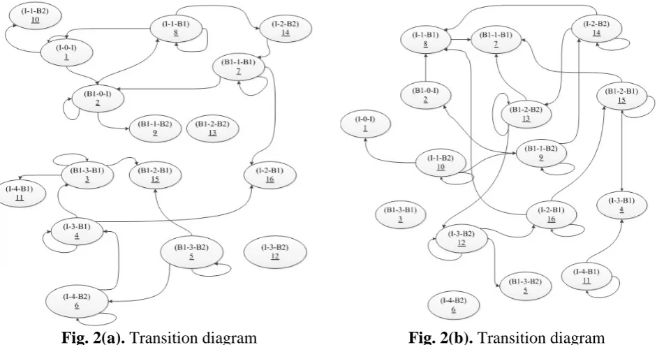
The transition diagram for the model of considered production system is shown in Fig. 2 (part a and b). To improve the readability of the transition diagram, it has been divided to two part that each part shows some transition arc of the system.
Fig. 2(a). Transition diagram Fig. 2(b). Transition diagram
In the following transition probability matrix all states and their probabilities are shown .The summation of each row must be one.
Transition Probability Matrix
States 1 2 3 4 5 6 7 8 9 10 11 12 13 14 15 16
1 1-γ- λ γ 0 0 0 0 0 0 0 λ 0 0 0 0 0 0
2 0 1-α–λ 0 0 0 0 0 α λ 0 0 0 0 0 0 0
3 0 0 1-α-β1 0 0 0 0 0 0 0 α 0 0 0 β1 0
4 0 0 γ 1-γ-β1 0 0 0 0 0 0 0 0 0 0 0 β1
5 0 0 0 0 1-α-β2 α 0 0 0 0 0 0 0 0 β2 0
6 0 0 0 β2 1- β2 0 0 0 0 0 0 0 0 0 0
7 0 β1 0 0 0 0 1- β1- α 0 0 0 0 0 0 0 0 α
8 β1 0 0 0 0 0 Γ 1- β1- γ 0 0 0 0 0 0 0 0
9 0 β2 0 0 0 0 0 0 1- β2- α 0 0 0 0 α 0 0
10 β2 0 0 0 0 0 0 0 Γ 1- β2- γ 0 0 0 0 0 0
11 0 0 0 β1 0 0 0 0 0 0 1-β1 0 0 0 0 0
12 0 0 0 0 γ 0 0 0 0 0 0 1- β2- γ 0 0 0 β2
13 0 0 0 0 0 0 β 2 0 0 0 0 α 1- β2- α 0 0 0
14 0 0 0 0 0 0 0 β 2 0 0 0 0 γ 1- β2- γ 0 0
15 0 0 0 α 0 0 β1 0 0 0 0 0 0 0 1- β1- α 0
16 0 0 0 0 0 0 0 β1 0 0 0 0 0 0 γ 1- β1- γ
The matrix were filled based on the states and their probabilities. For example we explained one state as follows:
It goes to state three (B1, 3, B1), if another Job one releases to system (with the probability of γ).
It remains in its state (I, 3, B1), if another Job one does not releases to and Station 2 still is working on Job one. So, all conditions occur with the probability of (1-β1-γ).
It goes to state sixteen (I, 2, B1), if Station 2 completes the operation on Job one (with the probability of β1, Imax = 2).
In the next section, we will calculate the transition probability with the assumed input of the job shop system and apply the DBR material flow management with a Markov chain analysis to compare traditional method with DBR.
4. Traditional approach to handling the production system
The predefined probability (α, β1, β2, γ, λ) are calculated in (Table 2). See Miltenburg (1997). For
calculation of probabilities some assumption are considered:
(1) Planning period is 1000 hours.
(2) In production plan 240 units of Job one and 140 units of Job two are produced. (3) Production time at Station 1 for Job one is four hours for each unit.
(4) Production time at Station 2 for Job one is six hours for each unit. (5) Production time at Station 2 for Job two is four hours for each unit.
The following occurrences are expected to happen during an arbitrary length period (for example a period of 100 hours).
Table 2
Transition probability.
Event Frequency Probability
Station 1 completes the operation of Job one(α) 100/4=25 25/235=0.106
Station 2 completes the operation of Job one(β1) (100/10)×(6/10)=6 6/235=0.025
Station 2 completes the operation of Job two(β2) (100/10)×(4/10)=4 4/235=0.017
Job one releases to the production line(γ) 100 100/235=0.0.425
Job two releases to the production line(λ) 100 100/235=0.0.425
Total=235 total≈1
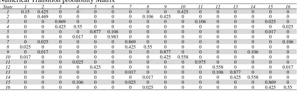
Now, we can calculate the numerical transition probability matrix base on the attained probability.
Numerical Transition probability Matrix
State 1 2 3 4 5 6 7 8 9 10 11 12 13 14 15 16
1 0.15 0.425 0 0 0 0 0 0 0 0.425 0 0 0 0 0 0
2 0 0.469 0 0 0 0 0 0.106 0.425 0 0 0 0 0 0 0
3 0 0 0.869 0 0 0 0 0 0 0 0.106 0 0 0 0.025 0
4 0 0 0.425 0.55 0 0 0 0 0 0 0 0 0 0 0 0.025
5 0 0 0 0 0.877 0.106 0 0 0 0 0 0 0 0 0.017 0
6 0 0 0 0.017 0 0.983 0 0 0 0 0 0 0 0 0 0
7 0 0.025 0 0 0 0 0.869 0 0 0 0 0 0 0 0 0.106
8 0.025 0 0 0 0 0 0.425 0.55 0 0 0 0 0 0 0 0
9 0 0.017 0 0 0 0 0 0 0.877 0 0 0 0 0.106 0 0
10 0.017 0 0 0 0 0 0 0 0.425 0.558 0 0 0 0 0 0
11 0 0 0 0.025 0 0 0 0 0 0 0.975 0 0 0 0 0
12 0 0 0 0 0.425 0 0 0 0 0 0 0.558 0 0 0 0.017
13 0 0 0 0 0 0 0.017 0 0 0 0 0.106 0.877 0 0 0
14 0 0 0 0 0 0 0 0.017 0 0 0 0 0.425 0.558 0 0
15 0 0 0 0.106 0 0 0.025 0 0 0 0 0 0 0 0.869 0
16 0 0 0 0 0 0 0 0.025 0 0 0 0 0 0 0.425 0.55
This matrix is called P and each cell of it is pij(transition probability from state i to state j). We define
some notation and then calculate them for our Markov chain as follows. See Miltenburg (1997).
{ }
πjΠ = ,
1 n
j i ij
i
p
π π
=
=
∑
× ,1
1
n
j j
π
=
=
∑
(1)Π = [0.000014 0.0006 0.1653 0.0509 0.0015 0.0096 0.0112 0.0005 0.0021 0.000013 0.7005 0.0004 0.0018 0.0005 0.0495 0.0055]
{ }
ijZ = z , Fundamental matrix. We need only the diagonal entries, so we write it here.
{ }
(
)
1ij
Z = z = − +I P A − (2)
Zjj = [1.2123 2.3019 5.6453 1.9548 8.0452 57.5257 10.0337 2.5039 9.4424 2.3125
5.4840 2.2443 8.2654 2.3236 9.4581 2.8195]
I = Unit matrix. B=
{ }
bj = The limiting variance for the number that the Markov chain is in each state;(
2 1)
j j jj j
b =π z − −π (3)
B = [0.000019 0.0022 1.6735 0.1456 0.0222 1.0995 0.2134 0.0019 0.0383 0.000048 6.4919 0.0015 0.0276 0.0019 0.8848 0.0254]
Before calculating the distribution of the number of units that are produced for each job we determine three sets from the Markov chain as follows:
Set 1 = the states of Markov chain that Job one is at Station 1 (number of states: 2, 3, 5, 7, 9, 13, and 15). Set 2 = the states of Markov chain that Job one is at Station 2 (number of states: 3, 4, 7, 8, 11, 15, and 16). Set 3 = the states of Markov chain that Job two is at Station 2 (number of states: 5, 6, 9, 10, 12, 13, and 14). The number of units that are produced in a period of transition (for Job one and two) has a normal distribution (mean is
∑
πj∈set RT and variance is 2j
b ∈set RT
∑
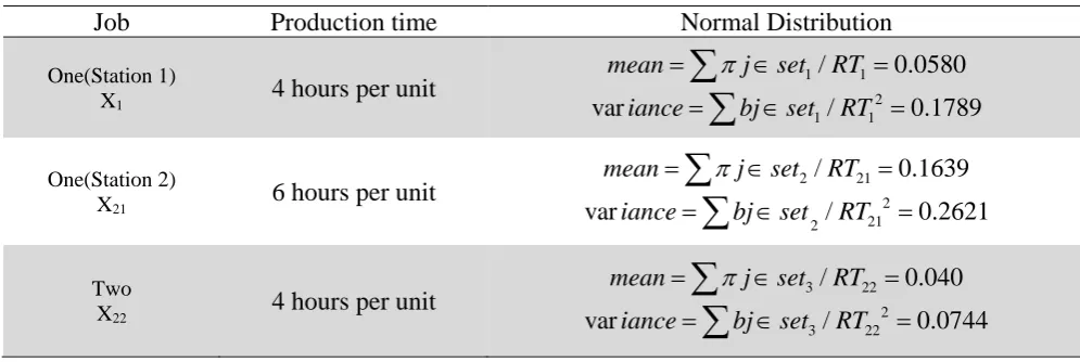
, here RT is the Production time at each Station on each Job) and is calculated in (Table 3). See Kemeny and Snell (1960) and Miltenburg (1997).Table 3
Production time distribution
Job Production time Normal Distribution
One(Station 1)
X1 4 hours per unit
1/ 1 0.0580
mean=
∑
πj∈set RT =2
1 1
variance=
∑
bj∈set /RT =0.1789One(Station 2)
X21 6 hours per unit
2/ 21 0.1639
mean=
∑
πj∈set RT =2 21 2
variance=
∑
bj∈set /RT =0.2621Two
X22 4 hours per unit
3/ 22 0.040
mean=
∑
π j∈set RT =2 3 22
variance=
∑
bj∈set /RT =0.07444.1Throughput
The number of units of Job one produced over the production planning period has following mean and variance:
The 95% interval estimate is = 163.9±1.96×16.18 = (140.2782, 195.6128)
The number of units of Job two that produced over the production planning period has following mean and variance:
Mean = 1000×mean of the number of units that are produced for Job two = 1000×0.040 = 40
Variance = 1000× variance of the number of units that are produced for Job two = 1000× 0.0744 = 74.4 The 95% interval estimate is = 40±1.96×8.62 = (23.1, 56.89)
4.2Shortage
Shortage is a situation where demand for a product exceeds the available output.
21 21 21
( ) ( ) ( ) _
pp
E shortage pp x f x dx pp production plan
−∞
=
∫
− = (4)After some steps we have:
( ) ( ) ( ( )z z ( ))
E shortage =σ Throughput × f s +sF ≤ s (5)
while
( ( )) ( )
s= pp−E Throughput σ Throughput (6)
z
f and Fz= unit normal distribution (See Miltenburg, 1997).
For Job one: 240 163.9 4.703 16.18
s= − =
( ) 16.18 ( z(4.703) 4.703 z (4.703)) 76.09
E shortage = × f + F ≤ =
For Job two: 140 40 11.6 8.62
s= − =
( ) 8.62 ( z(11.6) 11.6 z (11.6)) 100.76
E shortage = × f + F ≤ =
4.3 Work-in-process
Work-in-process are items that are waiting for further processing in a queue or a buffer inventory. To calculation the mean and variance of the Work-in-process, first we have to consider the inventory in the production line in each state:
State 1=0, State 2=0, State 3=3, State 4=3, State 5=3, State 6=4, State 7=1, State 8=1, State 9=1, State 10=1, State 11=4, State 12=3, State 13=2, State 14=2, State 15=2 and State 16=2.
16
1
3.623 j j
j
Mean I π
=
=
∑
= (7)16
2
1
( j ( )) j 0.43
j
Variance I E I π
=
=
∑
− = (8)4.4 Cycle time
Cycle time is the period required to complete a job from start to finish. In the proposed production system cycle time is the time at Station 1 adding to the time at Station 2 for Job one and is the time at Station 2 for Job two.
1 21
Jobone =(1 E X( )) (( ( ) 1)+ E I − E X( ))=33.244hours (9)
22
1 ( ) 25
two hours
5. DBR approach to handling the production system
DBR uses the drum or constraint to create a schedule based on the bottleneck. In the proposed production line Station 2 is the bottleneck of the system (its production time is larger than Station 1). Buffer which protects the constraint and the rope is a communication device that connects the constraint to the first Station. So, we use the buffer management to improve the measurement parameters (Fig. 3).
Rope
Fig. 3. A job shop production system with DBR management.
When the inventory in the production system deceases to one or zero and Station 2 is in the starvation danger, production time in Station 1 reduces the production time to 2.5 hours. When the inventory in the production system is more than one and Station 1 is in the danger to be blocked, production time in Station 2 reduces the production time to 5 hours for Job one and to 3 hours for Job two. So, again the Markov chain parameters and its calculation is shown in (Table 4).
Table 4
Transition Probability
Event Frequency I=0,1 (Probability) Frequency I=2,3,4 (Probability)
α 100/2.5=40 (40/250=0.16) 100/4=25 (25/238=0.105)
β1 (100/10)×(6/10)=6 (6/250=0.024) (100/8)×(5/8)≈8 (8/238=0.034)
β2 (100/10)×(4/10)=4 (4/250=0.016) (100/8)×(3/8)≈5 (5/238=0.021)
γ 100 (100/250=0.4) 100 (100/238=0.42)
λ 100 (100/250=0.4) 100 (100/238=0.42)
Now, we can calculate the numerical transition probability matrix based on the attained probability and the inventory in their states.
Numerical transition probability matrix
State 1 2 3 4 5 6 7 8 9 10 11 12 13 14 15 16
1 0.2 0.4 0 0 0 0 0 0 0 0.4 0 0 0 0 0 0
2 0 0.44 0 0 0 0 0 0.16 0.4 0 0 0 0 0 0 0
3 0 0 0.861 0 0 0 0 0 0 0 0.105 0 0 0 0.034 0
4 0 0 0.42 0.546 0 0 0 0 0 0 0 0 0 0 0 0.034
5 0 0 0 0 0.874 0.105 0 0 0 0 0 0 0 0 0.021 0
6 0 0 0 0.021 0 0.979 0 0 0 0 0 0 0 0 0 0
7 0 0.024 0 0 0 0 0.816 0 0 0 0 0 0 0 0 0.16
8 0.024 0 0 0 0 0 0.4 0.576 0 0 0 0 0 0 0 0
9 0 0.016 0 0 0 0 0 0 0.824 0 0 0 0 0.16 0 0
10 0.016 0 0 0 0 0 0 0 0.4 0.584 0 0 0 0 0 0
11 0 0 0 0.034 0 0 0 0 0 0 0.966 0 0 0 0 0
12 0 0 0 0 0.42 0 0 0 0 0 0 0.559 0 0 0 0.021
13 0 0 0 0 0 0 0.021 0 0 0 0 0.105 0.874 0 0 0
14 0 0 0 0 0 0 0 0.021 0 0 0 0 0.42 0.559 0 0
15 0 0 0 0.105 0 0 0.034 0 0 0 0 0 0 0 0.861 0
16 0 0 0 0 0 0 0 0.034 0 0 0 0 0 0 0.42 0.546
We calculate all predefined matrix to can compare them with each other.
1 1
, 1
ij
n n
j i j
i j
p
π π π
= =
=
∑
∑
=Π = [0.00004 0.0009 0.1960 0.0648 0.0023 0.01665 0.0187 0.0013 0.0021 0.000004 0.5975 0.0006 0.0027 0.0008 0.0836 0.0115]
{ }
(
)
1ij
Z = z = I− +P A − , Fundamental matrix. We need only the diagonal entries, so we write it here.
Station 1 Station 2
Zjj = [1.2921 2.0585 4.8873 1.8372 7.8175 46.0817 7.5439 2.7246 6.1967 2.4575
6.7840 2.2403 7.9854 2.3044 8.9619 2.9805]
I = Unit matrix.B=
{ }
bj =The limiting variance for the number that the Markov chain is in each state;(
2 1)
j j jj j
b =π z − −π
B = [0.0001 0.0028 1.6814 0.1691 0.0337 1.5176 0.2631 0.0058 0.0239 0.0002 7.1523 0.0021 0.0404 0.0029 1.4078 0.0569]
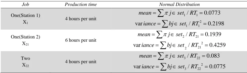
The number of units that are produced in a period of transition (for Job one and two) has a normal distribution (mean is
∑
πj∈set RT and variance is∑
bj∈set RT2, here RT is the weighted mean of production time base on the probability of amount of inventory) and is calculated in (Table 5).RT1 = 2.5×(probability that inventory is 0 or 1) +4×(probability that inventory is 2, 3 or 4) = 3.9635
RT21 = 6×(probability that inventory is 0 or 1) +5×(probability that inventory is 2, 3 or 4) = 5.0207
RT22 = 4×(probability that inventory is 0 or 1) +3×(probability that inventory is 2, 3 or 4) = 3.0217
Table 5
Production time distribution
Job Production time Normal Distribution
One(Station 1) X1
4 hours per unit 1 1
/ 0.0773
mean=
∑
πj∈set RT =2
1 1
variance=
∑
bj∈set /RT =0.2198One(Station 2) X21
6 hours per unit
2/ 21 0.1939
mean=
∑
πj∈set RT =2 21 2
variance=
∑
bj∈set /RT =0.4259Two X22
4 hours per unit
3/ 22 0.083
mean=
∑
π j∈set RT =2 3 22
variance=
∑
bj∈set /RT =0.07755.1. Throughput
Mean = 1000×mean of the number of units that are produced for Job one = 1000×0.1939=193.9 unit Variance = 1000× variance of the number of units that are produced for Job one = 1000× 0.2198 = 219.8 The 95% interval estimate is = 193.9 ±1.96×14.82 = (164.85, 222.94)
The number of units of Job two that produced over the production planning period has following mean and variance:
Mean = 1000×mean of the number of units that are produced for Job two = 1000×0. 083 = 83
Variance = 1000×variance of the number of units that are produced for Job two = 1000×0.0775 = 77.5 The 95% interval estimate is 83±1.96×8.803 = (65.74, 100.25)
5.2. Shortage
22 22 22
( ) ( ) ( ) _
pp
E shortage pp x f x dx pp production plan
−∞
=
∫
− =After some steps we have (E shortage)=σ(Throughput) (× f sz( )+sFz ≤( )),s while
( ( )) ( ) ,
For Job two s=(140 83) 8.803− =6.475 E shortage( )=8.803 (× fz(6.47) 6.47+ Fz ≤(6.47))=85.57
5.3.Work in process
16 16
2
1 1
3.467 ( ( )) 0.59
j j j j
j j
Mean I π Variance I E I π
= =
=
∑
= =∑
− =5.4.Cycle time
In the proposed production system cycle time is the time at Station 1 adding to the time at Station two for Job one and is the time at Station 2 for Job two.
1 21
(1 ( )) (( ( ) 1) ( )) 25.718
one hours
Job = E X + E I − E X = and Jobtwo =1 E X( 22) 12.048= hours
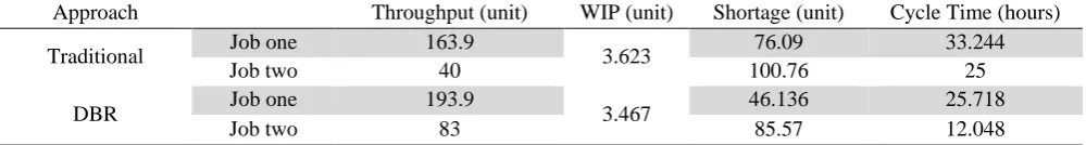
5.5.Comparison
The results are summarized in (Table 6). This table compares traditional and DBR approach to management of simple job shop production system. Some measurement parameters were considered.
Table 6
Comparison of two approaches.
Approach Throughput (unit) WIP (unit) Shortage (unit) Cycle Time (hours)
Traditional Job one 163.9 3.623 76.09 33.244
Job two 40 100.76 25
DBR Job one 193.9 3.467 46.136 25.718
Job two 83 85.57 12.048
It is clear that improvement by DBR is on all measurement parameters. While applying traditional approach is an easy approach to manage the production system, but in competition condition it cannot be a good approach. In competition environment, DBR gives the best competitive advantage.
6. Conclusions and future development
DBR develops production schedule by applying the first three steps in the TOC process. Many of papers did their researches and also their examples on DBR in the flow shop environment and scheduling job shop environment by DBR method is ignored, while many real production lines are job shop. This report applied the DBR technique in the job shop environment and used a Markov chain analysis to compare traditional method with DBR. Four measurement parameters were considered and the result showed the advantage of DBR approach in comparison to traditional approach. The present work showed the Markov chain analysis in handling first constraint resource by DBR technique. So, there is a scope for further research to extend a Markov chain analysis in a multiple constraint resources environment.
Acknowledgments
The authors would like to thank the anonymous reviewers of this paper for their thought-provoking and insightful comments and corrections.
References
Babu, T. R., Rao, K. S. P., & Maheshwaran, C. U. (2007). Application of TOC embedded ILP for increasing throughput of production lines. The International Journal of Advanced Manufacturing Technology, 33 (7-8), 812-818.
Betterton, C. E., & Cox, J. F. (2009). Espoused drum-buffer-rope flow control in serial lines: A comparative study of simulation models. International Journal of Production Economics, 117(1), 66-79.
Bozzone, V. (2002). The Theory of Delays, A Tool For Improving Performance And Profitability: In Job
Chakravorty, S. S. (2001). An evaluation of the DBR control mechanism in a job shop environment. Omega, 29(4), 335-342.
Chakravorty, S. S., & Atwater, J. B. (2005). The impact of free goods on the performance of drum-buffer-rope scheduling systems. International Journal of Production Economics, 95(3), 347-357.
Chakravorty, S. S., & Verhoeven, P. R. (1996). Learning the theory of constraints with a simulation game. Simulation & Gaming, 27(2), 223-237.
Chakravorty, S. S., & Verhoeven, P. R. (1996). Learning the theory of constraints with a simulation game. Simulation & Gaming, 27(2), 223-237.
Cheraghi, S. H., Dadashzadeh, M., & Soppin, M. (2011). Comparative analysis of production control systems through simulation. Journal of Business & Economics Research (JBER), 6(5), 87-104.
Georgiadis, P., & Politou, A. (2013). Dynamic Drum-Buffer-Rope approach for production planning and control in capacitated flow-shop manufacturing systems. Computers & Industrial Engineering, 65(4), 689-703.
Goldratt, E. (1997). Critical chain. Great Barrington, MA: North River Press.
Goldratt, E. (1988). Computerized shop floor scheduling. International Journal of Production Research,
26(3), 443-455.
Goldratt, E. (1990). What is this thing called theory of constraints and how should it be implemented?. Croton-on-Hudson, N.Y.: North River Press.
Goldratt, E., & Fox, R. (1986). The race. Croton-on-Hudson, NY: North River Press.
Grinstead, C., Snell, J., & Snell, J. (1997). Introduction to probability. Providence, RI: American Mathematical Society.
Gupta, M. (2003). Constraints management--recent advances and practices. International Journal of
Production Research, 41(4), 647-659.
Gupta, M., & Snyder, D. (2009). Comparing TOC with MRP and JIT: a literature review. International
Journal of Production Research, 47(13), 3705-3739.
Kemeny, J., & Snell, J. (1960). Finite markov chains. Princeton, N.J.: Van Nostrand.
Lee, J., Chang, J., Tsai, C., & Li, R. (2010). Research on enhancement of TOC Simplified Drum-Buffer-Rope system using novel generic procedures. Expert Systems with Applications, 37(5), 3747-3754.
Miltenburg, J. (1997). Comparing JIT, MRP and TOC, and embedding TOC into MRP. International Journal
of Production Research, 35(4), 1147-1169.
Pegels, C., & Watrous, C. (2005). Application of the theory of constraints to a bottleneck operation in a manufacturing plant. Journal of Manufacturing Technology Management, 16(3), 302-311.
Radovilsky, Z. (1998). A quantitative approach to estimate the size of the time buffer in the theory of constraints. International Journal of Production Economics, 55(2), 113-119.
Rahman, S. (1998). Theory of constraints. International Journal of Operations & Production Management,
18(4), 336-355.
Rand, G. (2000). Critical chain: the theory of constraints applied to project management. International
Journal of Project Management, 18(3), 173-177.
Ray, A., Sarkar, B., & Sanyal, S. (2010). The TOC-Based algorithm for solving multiple constraint resources.
IEEE Transactions on Engineering Management, 57(2), 301-309.
Ray, A., Sarkar, B., & Sanyal, S. (2008). An improved theory of constraints. International Journal of
Accounting & Information Management, 16(2), 155-165.
Sale, M., & Inman, R. (2003). Survey-based comparison of performance and change in performance of firms using traditional manufacturing, JIT and TOC. International Journal of Production Research, 41(4), 829-844.
Schragenheim, E., & Boaz, R. (1990). The Drum-Buffer-Rope shop floor control. Production and Inventory
Management Journal, 31(3), 18-23.
Schragenheim, E. and Dettmer, H. (2000). Manufacturing at warp speed. Boca Raton, FL: St. Lucie Press. Steele, D., Philipoom, P., Malhotra, M., & Fry, T. (2005). Comparisons between drum–buffer–rope and
material requirements planning: a case study. International Journal of Production Research, 43(15), 3181-3208.