Impact of an observational time window on coupled data assimilation: simulation with a simple climate model

https://doi.org/10.5194/npg-24-681-2017 © Author(s) 2017. This work is distributed under the Creative Commons Attribution 3.0 License.

Impact of an observational time window on coupled data

assimilation: simulation with a simple climate model

Yuxin Zhao1, Xiong Deng1,2, Shaoqing Zhang3, Zhengyu Liu4,5, Chang Liu1,2, Gabriel Vecchi6, Guijun Han7, and Xinrong Wu7

1_{College of Automation, Harbin Engineering University, Harbin, 150001, China} 2_{GFDL-Wisconsin Joint Visiting Program, Princeton, NJ 08540, USA}

3_{Physical Oceanography Laboratory/CIMST, Ocean University of China and Qingdao National Laboratory for Marine}

Science and Technology, Qingdao, 266100, China

4_{Atmospheric Science Program, Department of Geography, Ohio State University, Columbus, OH 43210, USA}

5_{Laboratory for Climate and Ocean-Atmosphere Studies (LaCOAS), Department of Atmospheric and Oceanic Sciences,}

School of Physics, Peking University, Beijing, 100871, China

6_{Atmospheric and Oceanic Program, Princeton University, Princeton, NJ 08540, USA} 7_{National Marine Data and Information Service, Tianjin, 300171, China}

Correspondence to:Shaoqing Zhang ([email protected])

Received: 14 November 2016 – Discussion started: 13 January 2017

Revised: 21 April 2017 – Accepted: 21 September 2017 – Published: 17 November 2017

Abstract. Climate signals are the results of interactions of multiple timescale media such as the atmosphere and ocean in the coupled earth system. Coupled data assimilation (CDA) pursues balanced and coherent climate analysis and prediction initialization by incorporating observations from multiple media into a coupled model. In practice, an ob-servational time window (OTW) is usually used to collect measured data for an assimilation cycle to increase obser-vational samples that are sequentially assimilated with their original error scales. Given different timescales of charac-teristic variability in different media, what are the optimal OTWs for the coupled media so that climate signals can be most accurately recovered by CDA? With a simple coupled model that simulates typical scale interactions in the climate system and “twin” CDA experiments, we address this issue here. Results show that in each coupled medium, an opti-mal OTW can provide maxiopti-mal observational information that best fits the characteristic variability of the medium dur-ing the data blenddur-ing process. Maintaindur-ing correct scale in-teractions, the resulting CDA improves the analysis of cli-mate signals greatly. These simple model results provide a guideline for when the real observations are assimilated into a coupled general circulation model for improving climate analysis and prediction initialization by accurately

recover-ing important characteristic variability such as sub-diurnal in the atmosphere and diurnal in the ocean.

1 Introduction

usu-682 Y. Zhao et al.: Impact of an observational time window

ally different. When the observed data included in one or more components of the coupled system framework are as-similated, the observational information will be able to be transferred among different media through the coupled dy-namics so that all media gain consistent and coherent adjust-ments. Such an assimilation procedure is called coupled data assimilation (CDA), which can sustain the nature of multi-ple timescale interactions during climate estimation and pre-diction initialization (e.g., Zhang et al., 2007; Sugiura et al., 2008; Singleton, 2011), thus producing better climate analy-sis and prediction initialization and therefore improving the coupled models’ predictability (Yang et al., 2013). Zhang et al. (2007) developed the first CDA system in a fully coupled general circulation model, version 2 of the Geophysical Fluid Dynamics Laboratory Coupled Model (GFDL CM2). The National Centres for Environmental Prediction (NCEP) also started using coupled models to generate first-guess forecasts for their Climate Forecast System Reanalysis (CFSR, Saha et al., 2010). Despite the enormous benefits and demand for CDA, it remains both theoretically and technically challeng-ing to implement strong CDA in fully coupled models, in-cluding the estimation of the coupled model error covariance matrix and the huge computational costs (e.g., Han et al., 2013; Lu et al., 2015; Liu et al., 2016).

During the coupled data assimilation process, an obser-vational time window (OTW) is usually used to collect measured data in each medium for an assimilation cycle (e.g., Pires et al., 1996; Hunt et al., 2004; Houtekamer and Mitchell, 2005; Laroche et al., 2007) to increase observa-tional samples. As in Hunt et al. (2004), we expand the EnKF to include a time window in which the observations are treated as the exact assimilation times, even though their times are different in the window. That is, we just assume that all the collected data sample the “truth” variation at the assimilation time and will be sequentially assimilated with their original error scales. Thus the OTW is applied in a three-dimensional data assimilation fashion rather than a four-dimensional one. Apparently, while a large OTW pro-vides more observational samples at the assimilation time, the assimilation process blends more data from different times and may distort the variability being retrieved. Given the fact that climate signals are the results of interactions of multiple timescale media, correct variability retrieved for each medium so that correct scale interaction is maintained in CDA is particularly important for climate analysis and prediction initialization. In this study we attempt to answer the following two questions. (1) What is the impact of vary-ing OTWs for each coupled component within the coupled model framework on the quality of CDA? (2) Based on this impact, does an optimal OTW exist so that assimilation fit-ting has maximum observational information but minimum variability distortion?

With a simple conceptual coupled climate model and a se-quential implementation of the ensemble Kalman filter, this study first analyses the characteristic variability timescale of

each coupled medium and identifies the corresponding opti-mal OTW. Then the impact of an optiopti-mal OTW on the qual-ity of CDA and its linkage with the corresponding timescale of characteristic variability are investigated. The simple cou-pled model consists of three typical components, including the synoptic atmosphere (Lorenz, 1963) and the seasonal– interannual slab upper ocean (Zhang et al., 2012) coupling with the decadal deep ocean (Zhang, 2011a, b). Although the simple conceptual coupled model does not share the similar complex physics with a coupled general circulation model (CGCM), it does reasonably simulate the typical interactions between multiple timescale components in the coupled cli-mate system (see Zhang et al., 2013). The simple coupled model helps us understand the essence of the problem by revealing the relationship between the optimal OTWs and corresponding timescales of characteristic variability as well as their impact on CDA. The low-cost nature of the simple model also provides convenience for a large number of CDA experiments with different OTWs in optimal OTW detec-tion. The ensemble Kalman filter (e.g., Evensen, 1994, 2007; Whitaker and Hamill, 2002; Anderson, 2001, 2003) used in this study is the ensemble adjustment Kalman filter (EAKF, e.g., Anderson, 2001, 2003; Zhang and Anderson, 2003). Us-ing the EAKF with the simple coupled model, we first estab-lish a twin experiment framework. Within such a framework, the degree to which the state estimation based on a certain OTW recovers the truth is an assessment of the influence of the OTW on the quality of CDA. In such a way, the optimal OTW of each medium is detected and the impact of optimal OTWs on CDA is evaluated. We also discuss the influence of model bias on an optimal OTW through biased twin experi-ment setting.

This paper is organized as follows. Section 2 briefly de-scribes the simple conceptual coupled model, the ensem-ble adjustment Kalman filter, as well as the twin experiment framework including perfect and biased settings. Also with a simplest case, we first show the influence of OTWs on assim-ilation quality and its linkage with the timescale of character-istic variability in this section. Then Sect. 3 presents results on detection of the optimal OTWs for different media and the impact of optimal OTWs on CDA. The influence of realistic assimilation scenarios on optimal OTWs is discussed in Sect. 4. Finally, a summary and discussions are given in Sect. 5.

2 Methodology 2.1 The model

sim-ple model is based on Lorenz’s three-variable chaotic model (Lorenz, 1963) that couples with a slab upper ocean (Zhang et al., 2012) and a simple pycnocline predictive model (Gnanadesikan, 1999). Although very simple with low com-putational cost, in terms of multi-scale interaction inducing low-frequency climate signals, this model shares a funda-mental character with a CGCM, and it is very suitable for addressing the problem that is concerned here. And for the readers’ convenience, here we simply review some key as-pects of this conceptual coupled model. With all quantities being given in non-dimensional units, the governing equa-tions are

˙

X1= −σ X1+σ X2,

˙

X2= −X1X3+(1+C1ω) kX1−X2,

˙

X3=X1X2−bX3,

Omω˙=C2X2+C3η+C4ωη−Odω+Sm

+Sscos 2π t /Spd,

0η˙=C5ω+C6ωη−Odη, (1)

where X1, X2, and X3 represent the atmospheric model

states, while ωandη denote those for the upper and deep ocean, respectively. A dot above the variable denotes the time tendency. The atmosphere model states are the high-frequency variables, while the slab oceanic variable ω is of a lower frequency. To sustain the chaotic nature of the atmosphere in reality, the standard values of the parameters included in the atmospheric component (σ, k, and b) are set as 9.95, 28, and 8/3, respectively. In the equation ofω, the parameters Od andOm denote the damping coefficient

and heat capacity of the upper slab ocean, respectively. Due to the lower frequency of ω than that of the model states in the atmospheric components, the timescale of the upper slab ocean variable must be much slower than that of the atmospheric model states. Thus the damping rate parameter

(Od)should be much smaller than the heat capacity, namely, OdOm. Here following Lorenz’s idea (Lorenz, 1963),

the atmospheric timescale is defined as the typical time by which the atmosphere goes through an attractive lob as 1 non-dimensional time unit (TU)∼O(1). We set the param-eters (Om, Od)as (10,1), which show that the slab oceanic

variable’s timescale is ∼O(10), i.e., 10 times that of the atmospheric model states. While the Sm+Sscos 2πt/Spd

represents the external forcing, the parameter Spd denoting

the model seasonal cycle is set as 10 to make sure that the period of the external forcing is comparable with the upper slab ocean variables’ timescale. In this simple coupled model, the seasonal cycle is set as 10 TUs and thus a model year (decade) equals 10 (100) TUs. The parameters Ss

and Sm, denoting the magnitudes of the external forcing’s

seasonal cycle and annual mean, are insensitive to the coupled model and set as (1,10). The coefficients C1 and C2in the equations ofX2andωare used to implement the

coupling between the fast atmosphere model states and the

upper slab oceanic variable and are set as (0.1,1), whereC1

denotes the upper slab oceanic forcing on the atmosphere while C2 denotes the atmosphere forcing on the ocean. In

addition,C3andC4represent the deep oceanic forcing and

the nonlinear interaction between the upper and deep ocean. In order to make sure that the atmospheric forcing plays a dominant role in the upper slab ocean, the magnitudes of

C3 and C4 should be lower than that of C2 and both set

as 0.01. As in Zhang (2011a), the deep ocean model state variableη, denoting the anomaly of pycnocline depth in the deep ocean, is derived from the two-term balance model of the zonal-time mean pycnocline (Gnanadesikan, 1999). Within the equation ofη, the parameter 0is kept constant and the ratio of0andOddenotes the deep ocean variable’s

timescale. The timescale of the deep ocean variable is longer than that of the slab ocean, defined by the relative magnitude of 0 to Od (0 is set as 100). Similar to the

equation ofω, the coefficients C5 andC6denote the linear

slab oceanic forcing and the nonlinear interaction between the upper and deep ocean. Also, to guarantee that the linear interaction is dominant and the nonlinear interaction is weaker than that in the deep ocean model,C5andC6are set

as (1, 0.001). In summary, in this study the standard values of the parameters included in this simple coupled model

(σ, k, b, C1, C2, Od, Om, Sm, Ss, Spd, 0, C3, C4, C5, C6) are

set as (9.95, 28, 8/3, 0.1, 1, 1, 10, 10, 1, 10, 100, 0.01, 0.01, 1, 0.001; e.g., Zhang, 2011a, b; Zhang et al., 2012; Han et al., 2013, 2014).

Following the study of Han et al. (2014), the fourth-order Runge–Kutta time-differencing scheme is used in this pa-per to resolve this simple coupled model, and the time step equals 0.01 TU (1 TU=100 time steps).

Zhang (2011b) illustrated that, given the model parame-ters described above, the constructed simple coupled model can effectively simulate a fundamental feature of the real-world climate system in which different timescales inter-act with each other to develop climate signals. That is, the synoptic to decadal timescale signals are produced by the interactions between the transient atmosphere attractor, the slow slab ocean, and the even slower deep ocean (see Zhang, 2011a; Han et al., 2014). Again, although the simple cou-pled model does not have complex physics and cannot con-sider the issue of impact of localization and imbalance as in a CGCM, it can help us investigate the fundamental issue we want to address here more directly and clearly.

2.2 Ensemble coupled data assimilation

684 Y. Zhao et al.: Impact of an observational time window

the Kalman filter (Kalman, 1960; Kalman and Bucy, 1961) called the ensemble adjustment Kalman filter (EAKF, An-derson, 2001, 2003; Zhang and AnAn-derson, 2003; Zhang et al., 2007), which is a sequential implementation of the ensemble Kalman filter under an “adjustment” idea, is used to imple-ment the CDA scheme. The assumption of independence of observational error allows the EAKF to sequentially assimi-late observations into corresponding model states (Zhang and Anderson, 2003; Zhang et al., 2007). While the sequential implementation provides much computation convenience for data assimilation, the EAKF maintains as much of the non-linearity of background flows as possible (Anderson, 2001, 2003; Zhang and Anderson, 2003).

Based on the two-step implementation of the EAKF scheme (Anderson, 2001, 2003), the observational increment at an observation location is first computed. The observation is denoted asY at timet (simplyY instead ofYt)which has

the observation valueYoand standard deviationσ_yo(assumed to be Gaussian). Firstly, the reshaping of the model ensemble at the observation location,1Y0, is formulated as

1Yi0=

1Y_ip

q

1+r_k2

and rk=

σ_k,kp

σ_k,ko , (2)

whereirepresents the ensemble index andkdenotes the ob-servation index. σ_k,ko andσ_k,kp are the standard deviation of observation error and its prior estimated ensemble standard deviation, respectively, while rk is the corresponding ratio.

Ifrk >1 , the ensemble spread is largely reduced by the

ob-servation; otherwise, the ensemble remains close to the prior. The shift of the ensemble mean induced by the observation is computed by

¯

YU= Y

p

1+r_k2+

Yo

1+r_k−2. (3)

We can see that if the prior estimated ensemble standard de-viation is greater than that of the observation error, the en-semble mean shifts toward the observation value; otherwise, the ensemble mean remains close to the prior model ensem-ble meanYp. Then the observational increment induced by the observation valueYofor theit hensemble member at the

kt hobservation location is computed as

1Y_k,io =YU_k +1Yk,i0

−Y_k,iP

=





Yp_k

1+r_k2+

Y_ko

1+r_k−2

+ 1Y

p k,i q

1+r_k2 

−Y_k,iP . (4)

Once we get the observational increment at the observation location, then a least square fit is used to distribute the incre-ment over the relevant grid points impacted by the observa-tion using the covariance between the grid index j and the

observationk,c_j,kp , using

1Zi,j =

cp_j,k

(σ_k,kp )21Y

o k,i=

Cov(Zj, Yk)

(σ_k,kp )2 1Y

o

k,i, (5)

whereZ represents a certain state variable at the grid point

j. The term1Zi,j is the contribution of thekth observation

to theith ensemble member of the model state estimated at grid pointj. When an observation is available, Eq. (5) will be applied to implement CDA for state estimation in a straight-forward manner (Zhang et al., 2007; Zhang, 2011a).

Although many sophisticated inflation algorithms (e.g., Anderson, 2007, 2009; Li et al., 2009; Miyoshi, 2011) ex-ist for atmosphere data assimilation, the inflation scheme for a coupled model is a new subject due to the multiple-timescale nature of the system. Furthermore, trial-and-error experiments show that the usual form of inflation (e.g., only inflate the atmosphere model states or inflate all the model states equally) will lead to the analysis becoming unstable. Thus, in this paper, for simplicity and computational con-venience as well as concon-venience for comparison, no infla-tion is used in our assimilainfla-tion experiments, just as in Han et al. (2014).

2.3 Perfect and biased twin experiment setups

In this study, a perfect twin experiment framework and a bi-ased twin experiment framework are designed, respectively. In both perfect and biased twin experiments, a “truth” model using the standard parameter values listed in Sect. 2.1 is used to generate the “true” solution of the model states and pro-duce the observations sampling the “truth”. Starting from the initial condition (0, 1, 0, 0, 0), the “truth” model is firstly integrated forward for 10 000 TUs (i.e., 1000 model years) for sufficient spinup and then integrated forward for another 10 000 TUs to generate the “truth” model states. The obser-vations are produced by sampling the “truth” solution of the model states at an observational interval and superimposing with a white noise simulating the observational errors. As schematically shown in Fig. 1, all the observational intervals used in this study are assumed to be 1 time step (0.01 TU). Although in the real climate system, the oceanic observations are usually available less frequently than those in the atmo-sphere (that is, the oceanic observation interval is larger than that we set here), for this proof-of-concept study we will set the time interval of the oceanic observations as small as pos-sible. The standard deviations of the observational errors are 2 forX1,X2, andX3and 0.5 forω. Also, although the deep

ocean lacks observations in the real world, we conduct some observation simulation experiments forη(the standard devi-ation of the observdevi-ational error is 0.06 forη)in this concep-tual study.

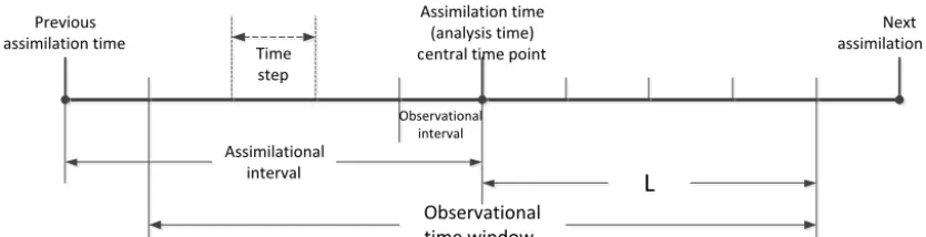
Assimilation time (analysis time) c entral time point

Next assimilation time Previous

assimilation time

Observational interval Assimilational

interval

L

time window

Time step

Figure 1.The schematic for the assimilation interval, the length of the OTW, as well as the observational interval in terms of the model integration time step. HereLrepresents the time steps at one side of the OTW. For example, OCN-OTW (L) in the content stands for an ocean observational time window with total observations of 2L+1.

model also uses the standard parameter values, but starts from different initial conditions using the Gaussian white noises with the same standard deviation as observational er-rors (2 forX1,X2, andX3, 0.5 forω, and 0.06 forη)added

to the model states at different times during the spinup run to form the ensemble initial conditions for each ensemble filter-ing data assimilation experiment. Each assimilation experi-ment is integrated for 10 000 TUs and only the data obtained in the last 5000 TUs are used to conduct error statistics for evaluation. We choose the model states between 9000 and 10 000 TUs during the spinup at an interval of 50 TUs being perturbed to form 20 cases of ensemble initial conditions for each assimilation experiment analyzed in Sects. 3 and 4. In this way, we attempt to minimize the dependence of the re-sults of optimal OTWs on ensemble initial states. Then each assimilation experiment will be repeated 20 times starting from these 20 independent ensemble initial conditions and we will analyze the mean value and uncertainty evaluated from these 20 cases.

Then we use the biased experiment setting to simulate the real-world scenario. The biased twin experiment frame-work is similar to the perfect one except that the assimilation model in the biased twin experiment framework has a sys-tematic discrepancy from the observations. Thus, in the bi-ased twin experiment framework, the parameters included in the assimilation model will have 10 % errors relative to the standard values. The errors in the parameters will be the only model error source.

Figure 1 also illustrates the assimilation update intervals (the assimilation intervals are 5 time steps for atmosphere, 20 time steps for the slab ocean in all assimilation experi-ments, and 100 time steps for the deep ocean when using theηobservations) as well as the length of the OTW, which will be used throughout the study. In addition, the coupling strength between the atmosphere and ocean may have influ-ences on the characteristic variability timescale of each cou-pled medium, such as on the optimal OTW. We discuss this issue by changing the values of coupling coefficientsC1and C2. In this simple model case, the model stability is

sensi-tive to the coupling coefficientC1(Zhang et al., 2012), and

changingC1only influences the chaotic component, so here

we just changeC2to investigate the impact of the coupling

coefficient between the atmosphere and upper ocean on the optimal OTWs. As in Zhang and Anderson (2003), an en-semble size of 20 is applied in all assimilation experiments in this study.

2.4 Influence of the OTW on the accuracy of CDA

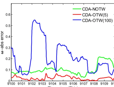
In order to exhibit the influence of the OTW on the qual-ity of climate analysis, we show three simple assimila-tion experiments (the time series of ω0s absolute errors) in Fig. 2: (1) standard CDA (green) (assimilating the ob-servation rights at the analysis times without any atmo-spheric/oceanic OTW); (2) OCN-OTW(5) CDA (red) (assim-ilating all 11 ocean observations in an oceanic OTW with a half-width of 5, defined as the length of the OTW here-after, but no atmospheric OTW is considered), and (3) OCN-OTW(100) CDA (blue) (assimilating all 201 ocean observa-tions in an oceanic OTW with a length of 100, but no atmo-spheric OTW is considered). The three assimilation experi-ments above are all conducted using the perfect model setting (all the parameters use their standard values) and the univari-ate adjustment scheme. The atmospheric and oceanic updunivari-ate intervals are 0.05 and 0.2 TU, respectively. While the stan-dard CDA does not use the atmospheric and oceanic OTWs and only assimilates the observations right at the analysis time, the OCN-OTW CDA incorporates all the valid obser-vations collected in the oceanic OTW. All three assimilation experiments above do not use an atmospheric OTW.

ap-686 Y. Zhao et al.: Impact of an observational time window

𝛚

9100 9101 9102 9103 9104 9105 9106 9107 9108 9109 91100

0.1 0.2 0.3 0.4 0.5 0.6

-a

bs

e

rr

or

Time step (TUs)

CDA-NOTW CDA-OTW(5) CDA-OTW(100)

Figure 2. Time series of the absolute errors of the slab ocean variable (ω)in three assimilation experiments based on the model states between 9100 and 9110 TUs assimilation results in the per-fect model experiment framework with the univariate adjustment scheme. Green – CDA control with the standard update intervals of 0.05 TU forX1,2,3and 0.2 TU forω; red – CDA with an ocean observational time window OTW) of five time steps (OCN-OTW (5)); blue – CDA with OCN-(OCN-OTW (100).

propriate OTW is used, we can gain optimal climate analysis. How can we determine such an optimal OTW? Next, starting from analyzing the characteristic variability of each coupled medium, we will discuss the methodology of how to deter-mine an optimal OTW for each medium in a coupled climate system.

2.5 The timescale of characteristic variability and an optimal OTW

The key to improving the accuracy of climate analysis in CDA is by accurately recovering the characteristic variabil-ity of different media in the coupled system. Thus we can assume that the length of an optimal OTW for each medium will have some relationship with the corresponding charac-teristic variability timescale. Then, we should first analyze the timescale of characteristic variability in each medium.

Figure 3 presents the power spectrum of X2 ω and η

based on the model states with a 4800 TU length (totally 480 000 data) after the spinup described in Sect. 2.3. From Fig. 3, we learned that in this simple model, the characteris-tic variability timescales of atmosphere (X2), upper ocean

(ω), and deep ocean (η) are about 1–2 TUs (1–2 model months), 50–100 TUs (5–10 model years), and 500 TUs (5 model decades), respectively. That is, the characteristic vari-ability timescale of the slab ocean is much larger than that of the atmosphere, but smaller than that of the deep ocean.

An optimal OTW aims to provide maximal observational information that best samples the characteristic variability of that medium during the data blending process. Thus the

length of the optimal OTW should be smaller than the cor-responding characteristic variability timescale, which means that the optimal OTW in the atmosphere must be much smaller than 1 TU (100 time steps), and in the ocean, the op-timal OTW must be much smaller than 50 TUs (5000 time steps). If we take observations for η, the optimal OTW for

ηmust be much smaller than 500 TUs (50 000 time steps). From Fig. 3, we also see that the characteristic variabil-ity timescales of different coupled media are a little larger than the corresponding ones set in Eq. (1). This is owing to the strong nonlinearity and smoothness of the fourth-order Runge–Kutta time-differencing scheme that prolongs the characteristic variability timescales of the simple coupled model. But they do not change the essence of the problem we address in this study. Given different timescales of character-istic variability in different media, in the following section we will further detect the optimal OTWs based on the cor-responding characteristic variability timescales and examine their impact on the quality of climate analysis in CDA.

3 Detection of the optimal observational time window

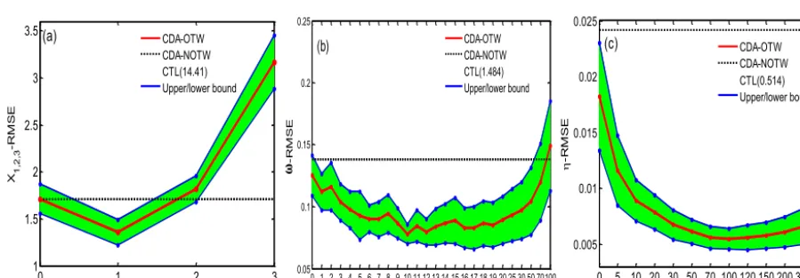
In this section, with the perfect model framework described in Sect. 2.3, we first conduct a series of CDA experiments with different ATM-OTWs and different OCN-OTWs to de-tect the optimal OTW for each medium. The assimilation scheme is the simple univariate adjustment scheme serving as a proof-of-concept study. To eliminate the dependency of results on initial states, each experiment is repeated 20 times starting from the 20 independent initial conditions described in Sect. 2.2. Then the mean value and the spread of 20 cases of RMSEs are plotted in Fig. 4.

Figure 4a shows that the optimal ATM-OTW is 1; i.e., the optimal ATM-OTW includes only three atmosphere ob-servations, with which the assimilation produces the lowest RMSE of the atmosphere and the smallest spread. (In this study each assimilation experiment will be repeated 20 times starting from 20 different independent initial ensemble con-ditions. Here the spread just represents the standard devia-tion of these 20 cases’ results. Thus it will be smallest when using the optimal OTW.) In these experiments for detecting the optimal ATM-OTW, the ocean assimilation is kept as the standard setting (i.e., no OTW, 0.2 TU update interval). Then we keep the ATM-OTW as 1 and change the length of OCN-OTW to produce Fig. 4b.

0 1 2 3 4 5 0

1 2

x 10-4

P

o

w

e

r-sp

e

c

tr

iu

m

-of

-X

2

Frequency (TU-1)

(a) Power-spectrum

95 %-confidence-upper-limit

0 0.2 0.4 0.6 0.8 1

0 0.005 0.01 0.015 0.02 0.025 0.03

P

o

w

e

r-s

p

e

c

tr

iu

m

-o

f-Frequency ((model year) -1)

(b) Power-spectrum

95 %-confidence-upper-limit

0 0.2 0.4 0.6 0.8 1

0 0.05 0.1 0.15 0.2

P

o

w

e

r-s

p

e

c

tr

iu

m

-o

f-

Frequency (decade-1)

(c) Power-spectrum

95 %-confidence-upper-limit

𝛚

Figure 3.The power spectrum (green) of(a)X2(b)ω, and(c)ηbased on the model states between 5000 and 9800 TUs integrations after the spinup which integrates for 10 000 TUs from the initial condition (0, 1, 0, 0, 0) with respect to the frequency, with 95 % statistical significance (red).

0 1 2 3

1 1.5 2 2.5 3 3.5

X1

,2

,3

-R

M

S

E

ATM-OTW (time steps)

(a) CDA-OTW

CDA-NOTW CTL(14.41) Upper/lower bound

0 1 2 3 4 5 6 7 8 9 10 11 12 13 14 15 16 17 18 19 20 25 30 50 70100 0.05

0.1 0.15 0.2 0.25

-R

M

S

E

OCN-OTW (time steps)

(b) CDA-OTW_CDA-NOTW

CTL(1.484) Upper/lower bound

0 5 10 20 30 50 70 100 120 150 200 300 400 0.005

0.01 0.015 0.02 0.025



-R

M

S

E

-OTW (time steps)

(c) CDA-OTW

CDA-NOTW CTL(0.514) Upper/lower bound

𝛚

Figure 4.Variations of root mean square errors (RMSEs) of(a)“atmospheric” statesX1,2,3(namely, the average ofX1,X2, andX3RMSEs) in the space of ATM-OTW length when the “oceanic” state (ω)only uses a single observation at the assimilation time;(b)“upper ocean” state (ω)in the space of OCN-OTW length when the ATM-OTW is fixed at 1 as shown in panel(a)(1 for the ATM-OTW, i.e., three observations in each window; see the caption of Fig. 1) but the OCN-OTW (forω)is varying and(c)“deep ocean” state (η)in the space ofη-OTW length when the “deep ocean” observations are assumed to be valid and the ATM-OTW and OCN-OTW are fixed as 1 and 10, respectively. The experiments are conducted in a perfect model setting with a simple univariate adjustment scheme. The red lines are the 20-case mean, each using different initial conditions taken from different periods in the control integration (see the description in Sect. 2.2), and the blue lines represent the upper/lower bounds (mean±standard deviations) of the RMSEs. An OTW with the length of 0 represents only assimilation of the observation at the assimilation time (i.e., with no OTW, dashed-black lines). The RMSE values of the control case (no observational constraint, called CTL) are marked in the parentheses.

OCN-OTW. (Because we just choose the optimal OCN-OTW from the figure ofω-RMSE. Thus in this study the variation of X-RMSEs in the OCN-OTW space is not shown.) This means that in this simple system, due to the strong nonlin-earity and chaotic nature of the “atmosphere”, the improved accuracy forωfrom optimal observational constraint is not sufficient to impact the “atmosphere” (this point will be ex-panded in Sect. 4.3). Similarly to the characteristic variabil-ity timescale of the slab ocean vs. that of the “atmosphere”

shown by Fig. 3, the optimal OCN-OTW is much larger than that of ATM-OTW.

688 Y. Zhao et al.: Impact of an observational time window

0 1 2 3 4 5 10 20 30 50 70 100

0 0.1 0.2 0.3 0.4 0.5 0.6 0.7 0.8

X 1

,2

,3

-en

se

m

bl

e sp

re

ad

ATM-OTW (time steps) (a)

CDA-OTW CDA-NOTW CTL(13.69) Upper/lower bound

0 5 10 15 20 25 30 50 70 100 150 200 250 300 400 500 0.005

0.01 0.015 0.02 0.025 0.03 0.035 0.04

-en

se

m

bl

e s

pr

ea

d

OCN-OTW (time steps)

(b) CDA-OTW

CDA-CDA-NOTW(0.06) CTL(1.406)

Upper/lower bound

𝛚

Figure 5.Same as panels(a)and(b)in Fig. 4 but for the variation of ensemble spreads of the model states. In panel(b)the optimal ATM-OTW is also set as 1. The area between the lower and upper bounds (blue) represents the range evaluated from the 20 cases. And the blue shadow below the ensemble spreads represents the range of the uncertainty of state estimation in each assimilation experiment.

observations), which is much larger than that of OCN-OTW and smaller than the characteristic variability timescale of the deep ocean pycnocline depth. With the optimalη-OTW, the RMSE ofηis reduced by about 77.4 % from the level of the CDA_NOTW.

We also check the variation of the 20-case mean ensemble spread in the space of OTWs as shown in Fig. 5. The mean and standard deviation of the ensemble spreads ofX1,2,3and ω (the uncertainty of the state estimation in each assimila-tion experiment is shown as the blue shadow in Fig. 5) grad-ually decrease when the ATM-OTW and OCN-OTW become larger. When the OTWs are set too large (here the ATM-OTW and OCN-ATM-OTW are greater than 20 and 250, respec-tively), the ensemble spreads of X1,2,3andωdecrease

dra-matically. This is owing to the fact that when we increase the length of the OTW, more observations will be included in the OTW and then assimilated into the corresponding model states, which can function as a smoother. The longer the lengths of OTWs are, the stronger the smoother will be. Also, under this circumstance, the overly strong smoother will dis-tort the characteristic variability of the model states, which explains the blue line of Fig. 2. From Figs. 4 and 5, we can see that the mean of the ensemble spread is significantly smaller than that of the corresponding RMSE. It is owing to the fact that no inflation scheme is applied in this study. And the statistics for evaluation are conducted from the data ob-tained in the last 5000 TUs. Thus after the first 5000 TUs’ assimilation in each assimilation experiment, the ensemble spreads of model states have been greatly reduced due to no inflation. Then the mean ensemble spread is significantly smaller than the mean RMSE.

To understand the essence of optimal OTWs, we show the auto-correlation for each model state and mark the time cor-relation coefficients at the timescales of optimal OTWs for

X2(a),ω(b), andη(c) detected from Figs. 4 to 6. The result

is the mean of 20 cases. In each case, the number of data are 10 000 steps (100 TUs), which are chosen from the period of

5000 to 9000 TUs in the truth run after spinup. From Fig. 6 we can see that all auto-correlations at the optimal OTW length are located at around 0.995. This means that the ob-servations included in an optimal OTW are extremely highly correlated with the model state at the analysis time. This can be understood since in this sequential assimilation scheme all the observations included in an OTW are assumed to be sam-pled at the analysis time so that the difference among them must be in a negligible range. Under such a circumstance, the optimal OTWs provide maximal observational informa-tion that best fits the characteristic variability and minimizes the analysis error.

4 Influences of realistic assimilation scenarios on optimal OTWs

In this section, we first show the impact of the multi-variate adjustment scheme on the optimal OTWs in a perfect model setting. Then we discuss the influence of model bias through a biased model framework. We will also investigate the im-pact of coupling strength on the optimal OTWs.

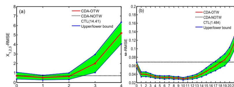
4.1 Influence of multi-variate adjustment on optimal OTWs

While the experiments with the univariate adjustment scheme provide us with a direct understanding of the influ-ence of the OTWs on CDA, we want to check whether or not it also applies to the multi-variate adjustment scheme. So we repeat the experiments described in Sect. 3 but with the multi-variate adjustment scheme. The results are shown in Fig. 7. Here the multi-variate adjustment scheme is only limited to the atmospheric observations (i.e., only the cross-covariances amongX1,X2, andX3are used; as indicated in

0 0.01 0.02 0.03 0.04 0.05 0.9 0.92 0.94 0.96 0.98 1 X -t im e c o rr e la ti o n c 2 o e ff ic ie n t

Time interval (TU) (a)

0 0.1 0.2 0.3 0.4 0.5 0.6 0.7

0.9 0.92 0.94 0.96 0.98 1 -t im e c o rr e la ti o n c o e ff ic ie n t

Time interval (TU) (b)

0 1 2 3 4 5 6 7

0.9 0.92 0.94 0.96 0.98 1  -t im e c o rr e la ti o n c o e ff ic ie n t

Time interval (TU) (c)

𝛚

Figure 6.The auto-correlation coefficient of(a)X2(b)ω, and(c)ηin the space of lag times are marked by corresponding time correlation coefficients at the timescale (L) of optimal OTWs as detected by Fig. 4 for different media (the black-dashed lines). What are shown are the means of 20 cases. In each case, an independent section (each has 10 000 data of the state – 100 TUs with the interval of 0.01 TU) is used to evaluate the lag correlation coefficient. The 20 independent sections are taken from the model states apart each 200 TUs between 5000 and 9000 TUs integrations after the spinup of 10 000 TUs from the initial condition (0, 1, 0, 0, 0).

0 1 2 3 4

0 1 2 3 4 5 6 7 8

X1,2

,3

-R

M

S

E

ATM-OTW (time steps)

(a) CDA-OTW

CDA-NOTW CTL(14.41) Upper/lower bound

0 1 2 3 4 5 6 7 8 9 10 11 12 13 14 15 16 17 18 19 20 25 30 0.02 0.04 0.06 0.08 0.1 0.12 0.14 0.16 0.18 0.2 -R M S E

OCN-OTW (time steps)

(b) _CDA-OTW

CDA-NOTW CTL(1.484) Upper/lower bound

𝛚

Figure 7.Same as Fig. 4 but using a multi-variate adjustment scheme. In panel(b)the optimal ATM-OTW is also set as 1.

the investigation of the problem we are addressing here). The results shown in Fig. 7 are similar to that in Fig. 4, suggest-ing the multi-variate adjustment scheme has little influence on the optimal OTWs, since it does not change the character-istic variability timescales (especially in this simple model).

The perfect experiment framework provides a direct guideline for the relationship between the optimal OTW and the corresponding characteristic variability timescale. How-ever, in reality, the numerical model has errors and is biased with the observation. It is as necessary to investigate the in-fluence of model bias on optimal OTWs as on the quality of CDA.

4.2 Influence of model bias on optimal OTWs

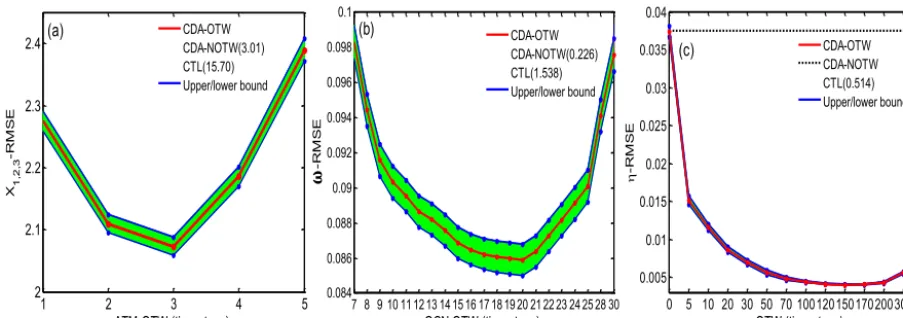
With the biased model experiment framework described in Sect. 2.3, we repeat all the experiments above for detection of the optimal OTWs. The results are shown in Fig. 8. Com-pared to the results in the perfect model setting, the results in

the biased model setting have two differences. First, the op-timal ATM-OTW and OCN-OTW are larger than their coun-terparts in the perfect model setting, becoming 3 and 20 (that is, the total observations are 7 and 41, respectively). Second, the RMSE curves in the space of OTWs show more concav-ity and sensitive variation. This is more distinguishable in the curve ofω-RMSEs in the OCN-OTW space. All these phe-nomena can be explained by the influence of model bias on the assimilation quality. On the one hand, due to the exis-tence of model bias, the assimilation not only needs vations to fit the observed variability, but also needs obser-vations to reduce the mean discrepancy between the model and observations. This requires stronger observational con-straints. An optimal OTW that makes the smallest RMSE of model states must include more observed data. On the other hand, the forecast ensemble in a biased model underestimates the forecast error, which results in the EAKF underweight-ing the observations. Therefore the optimal OTWs are larger

690 Y. Zhao et al.: Impact of an observational time window

1 2 3 4 5

2 2.1 2.2 2.3 2.4

X1

,2

,3

-R

M

S

E

ATM-OTW (time steps)

(a) CDA-OTW

CDA-NOTW(3.01) CTL(15.70) Upper/lower bound

7 8 9 10 11 12 13 14 15 16 17 18 19 20 21 22 23 24 25 28 30 0.084

0.086 0.088 0.09 0.092 0.094 0.096 0.098 0.1

-R

M

S

E

OCN-OTW (time steps)

(b) CDA-OTW

CDA-NOTW(0.226) CTL(1.538) Upper/lower bound

0 5 10 20 30 50 70 100120150170200300400 0.005

0.01 0.015 0.02 0.025 0.03 0.035 0.04



-R

M

S

E

-OTW (time steps)

(c) CDA-OTW

CDA-NOTW CTL(0.514) Upper/lower bound

𝛚

Figure 8.Same as Fig. 4 but using the biased model setting. In panel(b)the optimal ATM-OTW is set as 3. And in panel(c)the optimal ATM-OTW and OCN-OTW are kept as 3 and 20, when the “deep ocean” observations are assumed to be valid.

than those in the perfect experiment case in that the obser-vations included in the optimal OTWs will be assimilated for multiple times, which results in an improvement of fil-ter performance. The test experiment for the optimalη-OTW is also consistent with this point (in Fig. 8c): the optimalη -OTW in the biased model setting is larger than that in the perfect model setting. Then we also investigate the influence of OTWs on the quality of CDA with the multi-variate ad-justment scheme in the biased experiment framework (not shown here). The results are the same as the perfect model setting case; i.e., the multi-variate adjustment scheme does not change the optimal OTWs.

Comparing the results from two experiment frameworks, we can see that regardless of perfect or biased model setting used in the assimilation experiments, the optimal OTW must be associated with the corresponding characteristic variabil-ity timescale in the medium. It is clear that while using ob-servations in an OTW increases observational information, an overly large OTW can distort the characteristic variability of coupled media during the information blending process. Therefore choosing an optimal OTW that is much smaller than the medium’s characteristic variability timescale is very important. The simple model results suggest that the length of an optimal OTW is about 1–5 % of the medium charac-teristic timescale, with which characcharac-teristic variability of the medium can be retrieved most accurately.

In this study, the OTW validates the observations in a time window to the analysis time and all the observations included in the OTW are sequentially assimilated with their original error scales. Another general approach is to assimilate the average of the observations included in the OTW, but the ob-servational errors decrease as 1/

√

N of their original error scales (N represents the number of observations included in the OTW). From the comparison of these two methods (not shown), we can see that the results obtained by them are al-most the same. From the perspective of the calculation

pro-cess of the EAKF method, owing to no inflation scheme be-ing used, after many assimilation steps the ensemble spreads of the model states have been greatly reduced and are sig-nificantly smaller than the corresponding observational error scales. And the prior ensemble member will be very close to the prior ensemble mean. Thus the analysis adjustments obtained by these two methods will be almost the same. It is worth mentioning that although the resulting RMSEs ob-tained by these two assimilation schemes will be different when using the suitable inflation schemes, the lengths of the optimal OTWs are still the same and the essence of this study is still firm and does not change.

0 1 2 3 4 5 0

1 2

x 10-4

P

o

w

e

r-sp

e

c

tr

iu

m

-of

-X

2

Frequency (TU )-1

(a) Power-spectrum-1.5

Power-spectrum-1.25 Power-spectrum-1 Power-spectrum-0.8 Power-spectrum-0.5 Power-spectrum-0.1 95 %-confidence-upper-limit

0 0.2 0.4 0.6 0.8 1 1.2

0 0.005 0.01 0.015 0.02

P

o

w

e

r-s

p

e

c

tr

iu

m

-o

f-Frequency ((model year)-1)

(b) Power-spectrum-1.5Power-spectrum-1.25

Power-spectrum-1 Power-spectrum-0.8 Power-spectrum-0.5 Power-spectrum-0.1 95 %-confidence-upper-limit

50005010 5020 5030 5040 50505060 5070 5080 5090 51006

8 10 12 14 16 18

TU

(c) 1.5 1.25 1.0

0.8 0.5 0.1

𝛚

𝛚

Figure 9.The power spectrum of(a)X2and(b)ωbased on the model states between 5000 and 9800 TUs integrations after the spinup which integrates for 10 000 TUs from the initial condition (0, 1, 0, 0, 0) with different coupling strengths (C2is set as 1.5, 1.25, 1.0, 0.8, 0.5, and 0.1, whileC1remains as 0.1). Panel(c)shows the time series of the model stateωbetween 5000 and 5100 TUs integrations corresponding to the six cases.

0 1 5 10 15 16 17 18 19 20 21 22 23 24 25 26 27 28 29 30 31 32 33 34 35 40 50 70 100120150200300 0.05

0.1 0.15 0.2 0.25 0.3

-R

M

S

E

OCN-OTW (time steps)

(a) 1.5 1.25 1.0

0.8 0.5 0.1

0 0.1 0.2 0.3 0.4 0.5 0.6 0.7 0.8 0.9 1 1.1 1.2 1.3 1.4 1.5

10 20 30 40 50 60 70 80 90 100

Le

ng

th

-o

f-op

tim

al

-O

C

N

-O

T

W

C2

(b) Length of the optimal OCN-OTW

𝛚

Figure 10.Panel(a)is the same as panel(b)in Fig. 9 but for using six different coupling strength cases (withC2values of 1.5, 1.25, 1.0, 0.8, 0.5, and 0.1, whileC1stays as 0.1). Panel(b)is the variation of the length of the optimal OCN-OTW with respect to the values ofC2.

be obvious and the weights of the observations will be very necessary. But from this simple model case, we can see that regardless of using the weighted observations, the relation-ship between the characteristic variability timescales and the optimal OTWs will be robust, and the essence of this study is established.

4.3 Influence of coupling strength on optimal OTWs

Changing the coupling strength (controlled by the coupling coefficientsC1andC2in this case) between the atmosphere

and upper ocean may have some influence on the character-istic variability timescales of coupled media, as on the op-timal OTWs. Test experiments show that changing the cou-pling coefficientC1has little influence on the characteristic

variability timescales of X1,2,3 andω. This is because the

characteristic timescale of X is determined by the chaotic

nature of the Lorenz equations, not by the oceanic forcing associated with the coupling coefficientC1. Therefore, here

we just changeC2to investigate the coupling coefficient

be-tween the atmosphere and upper ocean on the optimal OTW ofω. Setting the values ofC2as 1.5, 1.25, 1.0, 0.8, 0.5, and

0.1 and keepingC1as 0.1, we repeat all the biased CDA

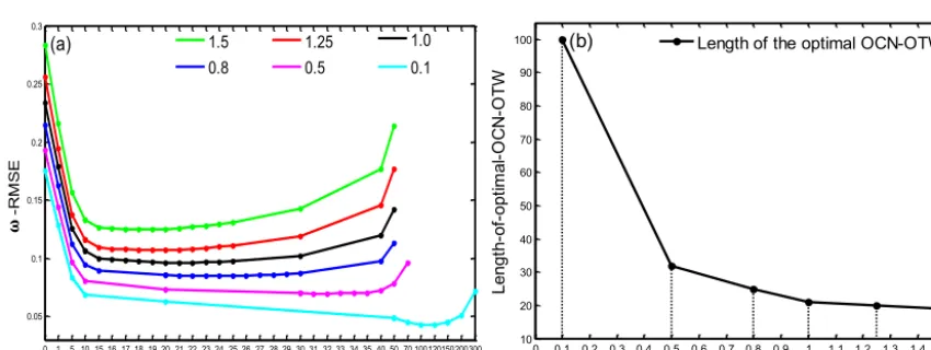
ex-periments with the multi-variate adjustment scheme. The re-sults are shown in Fig. 9, which presents the power spectrum ofX2andω(panels a and b) of the six cases above based

on the model states between 5000 and 9800 TUs, as well as the time series of model states between 5000 and 5100 TUs (panel c) after the spinup described in Sect. 2.3. We can see that changingC2 does not influence the characteristic

ex-692 Y. Zhao et al.: Impact of an observational time window

ternal forcing. WhenC2is small, the forcing of atmosphere

to ocean is weak, and then the periodic external forcing plays a dominant role in determining the characteristic variability timescale of the ocean component.

Then we examine the difference in the optimal OTW ofω

in the six cases above, as shown in Fig. 10. The results show that changingC2does not have any influence on the optimal

ATM-OTW (not shown). From panels a and b we can see that when C2 is smaller, the optimal OCN-OTW is larger.

This can be explained by the increasing role of the periodic external forcing in determining variability of the slab ocean, for which data assimilation needs more observational infor-mation to recover the periodic variation ofω, determined by the timescale defined bySpd(10 TU). WhenC2is larger than

1.0, changing it has little influence on the characteristic vari-ability of theω, as on the optimal OCN-OTW.

On the one hand, these experiments can further illustrate the idea that a close relationship between the length of the optimal OTW and the corresponding characteristic variabil-ity timescale exists. On the other hand, for a realistic CDA system, the coupling physics could be very complicated and affected by many factors. The results of this simple model give the insights that when determining the length of the op-timal OTWs for a realistic CDA system, we can only consider such factors that have an obvious influence on the character-istic variability timescales. In this way, the process of deter-mining the optimal OTWs in a realistic CDA system can be greatly simplified and make it possible to apply the method of using the optimal OTWs to the realistic CDA system.

5 Summary and discussions

With a simple conceptual climate model and the EAKF method, the impact of OTWs on the quality of CDA has been investigated in this study. This simple conceptual coupled model consists of a synoptic atmosphere (Lorenz, 1963) and seasonal–interannual slab upper ocean (Zhang et al., 2012) coupling with a decadal deep ocean (Zhang, 2011a, b), and reasonably simulates the typical interactions between multi-ple timescale components in the climate system. Determined from the characteristic variability timescale in each coupled medium, an optimal OTW provides maximal observational information to best fit the characteristic variability of the medium during the data blending process. With correct scale interactions within the coupled system, CDA can recover the climate signals most accurately by incorporating all observa-tions in the optimal OTWs into the coupled model, although in an idealized and simple model circumstance, the conclu-sion addressing the best fitting characteristic variability in each medium with the optimal OTW is comprehensive and therefore provides a guideline for improving climate analy-sis and prediction initialization when real observations are assimilated into a CGCM. For example, as learned from the simple model results, we may consider improving the quality

of climate analysis and prediction initialization by accurately recovering some important characteristic variability in the atmosphere (sub-diurnal variations, for instance) and ocean (diurnal cycle in the tropical oceans, for instance).

However, the current work can only serve as a proof-of-concept study. Although CDA with the optimal OTWs has shown promising improvement in this simple model, serious challenges still exist for detecting optimal OTWs in the real world with a CGCM for improving climate analysis and pre-diction. First, the characteristic variability timescales in dif-ferent media of the real world are complex, and great chal-lenges remain to identify the characteristic variability of the different component models and the real atmosphere and up-per and deep ocean, which need to be further studied. Also, in a real ocean model, the upper and deep ocean is inseparable, which bring some troubles in using different OTWs for dif-ferent parts of the same ocean model. Second, due to model biases, characteristic variability in a CGCM may be different from the real world. The combination of variability of the real world and that of the model may further complicate the problem. Therefore, model bias and its influence on model variability need to be thoroughly analyzed before an optimal OTW is determined. Thirdly, the coupling physics between different coupled components are very complicated and are impacted by many factors for a realistic CDA system. Even though we only consider the factors which will obviously im-pact the characteristic variability timescales when determin-ing the length of OTWs for different coupled components, it remains a heavy workload. In addition, in this study we as-sume that all observations in the OTWs have equal weights to contribute to the observational constraint. In the real obser-vation case, the obserobser-vation far away from the assimilation time should have less contribution to the state estimation at the assimilation time. How to take the time correlation into account in a sequential algorithm needs to be studied before implementing optimal OTWs in the assimilation with CGCM and real observations.

Data availability. Data can be obtained by contacting the author

Xiong Deng ([email protected]).

Competing interests. The authors declare that they have no conflict

of interest.

Acknowledgements. This work was supported by National

University and China Scholar Council (awarded to Xiong Deng for two and a half years’ study abroad at UW-Madison – NOAA/GFDL Joint Visiting Program). We thank Liwei Jia, Wei Zhang, Xue-feng Zhang, Wei Li, Lianxin Zhang, and Shuo Yang for their comments and suggestions on the early version of this manuscript. Also, special thanks to three anonymous reviewers for their critical comments that contributed to great improvements in the original manuscript.

Edited by: Amit Apte

Reviewed by: three anonymous referees

References

Anderson, J. L.: An ensemble adjustment Kalman Filter for data assimilation, Mon. Weather Rev., 129, 2884–2903, https://doi.org/10.1175/1520-0493(2001)129<2884:AEAKFF>2.0.CO;2, 2001.

Anderson, J. L.: A local least squares frame-work for ensemble filtering, Mon. Weather Rev., 131, 634–642, https://doi.org/10.1175/1520-0493(2003)131<0634:ALLSFF>2.0.CO;2, 2003.

Anderson, J. L.: An adaptive covariance inflation error correc-tion algorithm for ensemble filters, Tellus A, 59, 210–224, https://doi.org/10.1111/j.1600-0870.2006.00216.x, 2007. Anderson, J. L.: Spatially and temporally varying adaptive

co-variance inflation for ensemble filter, Tellus A, 61, 72–83, https://doi.org/10.1111/j.1600-0870.2008.00361.x, 2009. Chen, D., Zebiak, S. E., Busalacchi, A. J., and Cane, M. A.: An

im-proved procedure for EI Nino forecasting: implications for pre-dictability, Science, 269, 1699–1702, 1995.

Chen, D.: Coupled data assimilation for ENSO prediction, Adv. Geosci., 18, 45–62, 2010.

Collins, W. D., Blackman, M. L., Hack, J., Henderson, T. B., Kiehl, J. T., Large, W. G., and Mckenna, D. S.: The community climate system model version 3 (CCSM), J. Climate, 19, 2122–2143, https://doi.org/10.1175/JCLI3761.1, 2006.

Delworth, T. L., Broccoli, A. J., Rosati, A., et al.: GFDL’s CM2 Global Coupled Climate Models, Part I: Formula-tion and simulaFormula-tion characteristics, J. Climate, 19, 643–674, https://doi.org/10.1175/JCLI3629.1, 2006.

Evensen, G.: Sequential data assimilation with a nonlinear quasi-geostrophic model using Monte Carlo methods to fore-cast error statistics, J. Geophys. Res., 99, 10143–10162, https://doi.org/10.1029/94JC00572, 1994.

Evensen, G.: Data assimilation: The Ensemble Kalman Filter, Springer, 187 pp., 2007.

Gnanadesikan, A.: A simple predictive model for the structure of the oceanic pycnocline, Science, 283, 2077–2079, 1999. Hamill, T. M. and Snyder, C.: A hybrid ensemble Kalman

filter-3D variational analysis scheme, Mon. Weather Rev., 128, 2905–2919, https://doi.org/10.1175/1520-0493(2000)128<2905:AHEKFV>2.0.CO;2, 2000.

Han, G., Wu, X., Zhang, S., Liu, Z., and Li, W.: Error covariance es-timation for coupled data assimilation using a Lorenz atmosphere and a simple pycnocline ocean model, J. Climate, 26, 10218– 10231, https://doi.org/10.1175/JCLI-D-13-00236.1, 2013.

Han, G., Zhang, X., Zhang, S., Wu, X., and Liu, Z.: Mitigation of coupled model biases included by dynamical core misfitting through parameter optimization: simulation with a simple pycn-ocline prediction model, Nonlin. Processes Geophys., 21, 357– 366, https://doi.org/10.5194/npg-21-357-2014, 2014.

Hunt, B. R., Kalnay, E., Kostelich, E. J., Ott, E., Patil, D. J., Sauer, T., Szunyogh, I., Yorke, J. A., and Zimin, A. V.: Four-dimensional ensemble Kalman filtering, Tellus A, 56, 273–277, https://doi.org/10.1111/j.1600-0870.2004.00066.x, 2004. Houtekamer, P. L. and Mitchell, H. L.: Ensemble kalman

filtering, Q. J. Roy. Meteor. Soc., 131, 3269–3289, https://doi.org/10.1256/qj.05.135, 2005.

Kalman, R.: A new approach to linear filtering and prediction problems, Trans. ASME. Ser. D. J. Basic Eng., 82, 35–45, https://doi.org/10.1115/1.3662552, 1960.

Kalman, R. and Bucy, R.: New results in linear filtering and pre-diction theory, Trans. ASME. Ser. D. J. Basic Eng. 83, 95–109, https://doi.org/10.1115/1.3658902, 1961.

Laroche, S., Gauthier, P., Tanguay, M., Pellerin, S., and Morneau, J.: Impact of the different components of 4DVAR on the global forecast system of the Meteorological Ser-vice of Canada, Mon. Weather Rev., 135, 2355–2364, https://doi.org/10.1175/MWR3408.1, 2007.

Li, H., Kalnay, E., and Miyoshi, T.: Simultaneous estimation of covariance inflation and observation errors within an ensem-ble Kalman filter, Q. J. Roy. Meteor. Soc., 135, 523–533, https://doi.org/10.1002/qj.371, 2009.

Liu H., Lu, F., Liu, Z., Liu, Y., and Zhang, S.: Assimilating At-mosphere Reanalysis in Coupled Data Assimilation, J. Meteorol. Res., 30, 572–583, https://doi.org/10.1007/s13351-016-6014-1, 2016.

Lorenz, E. N.: Deterministic non-periodic flow, J. Atmos. Sci., 20, 130–141, 1963.

Lu, F., Liu, Z., Zhang, S., and Liu, Y.: Strongly Coupled Data Assimilation Using Leading Averaged Coupled Covariance (LACC). Part I: Simple Model Study, Mon. Weather Rev., 143, 3823–3837, https://doi.org/10.1175/MWR-D-14-00322.1, 2015. Miyoshi, T.: The Gaussian approach to adaptive covariance in-flation and its implementation with the local ensemble trans-form Kalman filter, Mon. Weather Rev., 139, 1519–1535, https://doi.org/10.1175/2010MWR3570.1, 2011.

Pires, C., Vautard, R., and Talagrand, O.: On extending the limits of variational assimilation in nonlinear chaotic systems, Tellus A, 48, 96–121, https://doi.org/10.1034/j.1600-0870.1996.00006.x, 1996.

Randall, D. A., Wood, R. A., Bony, S., Colman, R., Fichefet, T., Fyfe, J., Kattsov, V., Pitman, A., Shukla, J., Srinivasan, J., Stouf-fer, R. J., Sumi, A., and Taylor, K. E.: Climate models and their evaluation, Climate Change 2007: The physical Science Basis, edited by: Solomon, S., Qin, D., Manning, M., Chen, Z., Mar-quis, M., Averyt, K. B., Tignor, M., and Miller, H. L., Cambridge University Press, 589–662, 2007.

Saha, S., Moorthi, S., Pan, H.-L., et al.: The NCEP Climate Fore-cast System Reanalysis, B. Am. Meteor. Soc., 91, 1015–1057, https://doi.org/10.1175/2010BAMS3001.1, 2010.

694 Y. Zhao et al.: Impact of an observational time window

Sugiura, N., Awaji, T., Masuda, S., Mochizuki, T., Toyoda, T., Miyama, T., Igarashi, H., and Ishikawa, Y.: Development of a four-dimensional variation coupled data assimilation sys-tem for enhanced analysis and prediction of seasonal to in-terannual climate variations, J. Geophys. Res., 113, C10017, https://doi.org/10.1029/2008JC004741, 2008.

Whitaker, J. S. and Hamill, T. M.: Ensemble data assimi-lation without perturbed observations, Mon. Weather Rev., 130, 1913–1924, https://doi.org/10.1175/1520-0493(2002)130<1913:EDAWPO>2.0.CO;2, 2002.

Yang, X., Rosati, A., Zhang, S., Delworth, T. L., Gudgel, R. G., Zhang, R., Vecchi, G., Anderson, W., Chang, Y., DelSole, T., Dixon, K., Msadek, R., Stern, W. F., Wittenberg, A., and Zeng, F.: A predictable AMO-like pattern in GFDL’s fully coupled en-semble initialization and decadal forecasting system, J. Climate, 26, 650–661, https://doi.org/10.1175/JCLI-D-12-00231.1, 2013. Zhang, S. and Anderson, J. L.: Impact of spatially and tem-porally varying estimates of error covariance on assimila-tion in a simple atmospheric model, Tellus A, 55, 126–147, https://doi.org/10.1034/j.1600-0870.2003.00010.x, 2003. Zhang, S., Harrison, M. J., Rosati, A., and Wittenberg, A.: System

design and evaluation of coupled ensemble data assimilation for global oceanic climate studies, Mon. Weather Rev., 135, 3541– 3564, https://doi.org/10.1175/MWR3466.1, 2007.

Zhang, S.: Impact of observation-optimized model parameters on decadal predictions: simulation with a simple pycno-cline prediction model, Geophys. Res. Lett., 38, L02702, https://doi.org/10.1029/2010GL046133, 2011a.

Zhang, S.: A study of impacts of coupled model initial shocks and state-parameter optimization on climate predictions using a simple pycnocline prediction model, J. Climate, 24, 6210–6226, https://doi.org/10.1175/JCLI-D-10-05003.1, 2011b.

Zhang, S., Liu, Z., Rosati, A., and Delworth, T.: A study of en-hancive parameter correction with coupled data assimilation for climate estimation and prediction using a simple coupled model, Tellus A, 64, 1–20, https://doi.org/10.3402/tellusa.v64i0.10963, 2012.

Zhang, S., Winton, M., Rosati, A., Delworth, T., and Huang, B.: Impact of enthalpy-based ensemble filtering sea ice data as-similation on decadal predictions: simulation with a concep-tual pycnocline prediction model, J. Climate, 26, 2368–2378, https://doi.org/10.1175/JCLI-D-11-00714.1, 2013.