Atmos. Meas. Tech., 6, 511–526, 2013 www.atmos-meas-tech.net/6/511/2013/ doi:10.5194/amt-6-511-2013
© Author(s) 2013. CC Attribution 3.0 License.
EGU Journal Logos (RGB)
Advances in
Geosciences
Open Access
Natural Hazards
and Earth System
Sciences
Open AccessAnnales
Geophysicae
Open AccessNonlinear Processes
in Geophysics
Open AccessAtmospheric
Chemistry
and Physics
Open AccessAtmospheric
Chemistry
and Physics
Open Access DiscussionsAtmospheric
Measurement
Techniques
Open AccessAtmospheric
Measurement
Techniques
Open Access DiscussionsBiogeosciences
Open Access Open Access
Biogeosciences
DiscussionsClimate
of the Past
Open Access Open Access
Climate
of the Past
Discussions
Earth System
Dynamics
Open Access Open Access
Earth System
Dynamics
DiscussionsGeoscientific
Instrumentation
Methods and
Data Systems
Open Access
Geoscientific
Instrumentation
Methods and
Data Systems
Open Access DiscussionsGeoscientific
Model Development
Open Access Open Access
Geoscientific
Model Development
DiscussionsHydrology and
Earth System
Sciences
Open AccessHydrology and
Earth System
Sciences
Open Access DiscussionsOcean Science
Open Access Open Access
Ocean Science
DiscussionsSolid Earth
Open Access Open Access
Solid Earth
DiscussionsThe Cryosphere
Open Access Open Access
The Cryosphere
DiscussionsNatural Hazards
and Earth System
Sciences
Open Access
Discussions
Long-term greenhouse gas measurements from aircraft
A. Karion1,2, C. Sweeney1,2, S. Wolter1,2, T. Newberger1,2, H. Chen2, A. Andrews2, J. Kofler1,2, D. Neff1,2, and P. Tans2 1Cooperative Institute for Research in Environmental Sciences, University of Colorado, Boulder, Colorado, USA
2NOAA Earth System Research Laboratory, Boulder, Colorado, USA
Correspondence to: A. Karion (anna.karion@noaa.gov)
Received: 31 August 2012 – Published in Atmos. Meas. Tech. Discuss.: 2 October 2012 Revised: 7 February 2013 – Accepted: 11 February 2013 – Published: 1 March 2013
Abstract. In March 2009 the NOAA/ESRL/GMD Carbon
Cycle and Greenhouse Gases Group collaborated with the US Coast Guard (USCG) to establish the Alaska Coast Guard (ACG) sampling site, a unique addition to NOAA’s atmospheric monitoring network. This collaboration takes advantage of USCG bi-weekly Arctic Domain Awareness (ADA) flights, conducted with Hercules C-130 aircraft from March to November each year. Flights typically last 8 h and cover a large area, traveling from Kodiak up to Barrow, Alaska, with altitude profiles near the coast and in the interior. NOAA instrumentation on each flight in-cludes a flask sampling system, a continuous cavity ring-down spectroscopy (CRDS) carbon dioxide (CO2)/methane (CH4)/carbon monoxide (CO)/water vapor (H2O) analyzer, a continuous ozone analyzer, and an ambient temperature and humidity sensor. Air samples collected in flight are analyzed at NOAA/ESRL for the major greenhouse gases and a vari-ety of halocarbons and hydrocarbons that influence climate, stratospheric ozone, and air quality.
We describe the overall system for making accurate green-house gas measurements using a CRDS analyzer on an air-craft with minimal operator interaction and present an assess-ment of analyzer performance over a three-year period. Over-all analytical uncertainty of CRDS measurements in 2011 is estimated to be 0.15 ppm, 1.4 ppb, and 5 ppb for CO2, CH4, and CO, respectively, considering short-term precision, calibration uncertainties, and water vapor correction uncer-tainty. The stability of the CRDS analyzer over a seven-month deployment period is better than 0.15 ppm, 2 ppb, and 4 ppb for CO2, CH4, and CO, respectively, based on differ-ences of on-board reference tank measurements from a lab-oratory calibration performed prior to deployment. This sta-bility is not affected by variation in pressure or temperature during flight. We conclude that the uncertainty reported for
our measurements would not be significantly affected if the measurements were made without in-flight calibrations, pro-vided ground calibrations and testing were performed reg-ularly. Comparisons between in situ CRDS measurements and flask measurements are consistent with expected mea-surement uncertainties for CH4and CO, but differences are larger than expected for CO2. Biases and standard deviations of comparisons with flask samples suggest that atmospheric variability, flask-to-flask variability, and possible flask sam-pling biases may be driving the observed flask versus in situ CO2differences rather than the CRDS measurements.
1 Introduction
Quantifying greenhouse gas (GHG) emissions in the Arctic is crucial for understanding changes in the carbon cycle be-cause of their large potential impact on the earth’s warming. As organic carbon stored in thawing Arctic permafrost resur-faces, a portion of it will be emitted as either methane (CH4) or carbon dioxide (CO2). Because methane’s global warm-ing potential is more than 25 times greater than that of CO2 for a 100-yr time horizon (Forster, 2007), and because Arctic stores of organic carbon are estimated to be larger than the to-tal carbon from anthropogenic emissions since the beginning of the industrial era, Arctic CH4 emissions will potentially create an important feedback mechanism for climate change (McGuire et al., 2009; Jorgenson et al., 2001; Keyser et al., 2000; O’Connor et al., 2010). An understanding of how the permafrost thaw evolves is of paramount importance.
establish a new airborne sampling program over Alaska. The USCG Air Station Kodiak regularly conducts Arctic Domain Awareness (ADA) flights, using their fleet of four C-130 Her-cules aircraft for routine monitoring of the melting sea ice and changing conditions around Alaska. The NOAA aircraft group collaborated with the USCG to install an atmospheric sampling payload aboard the aircraft slated for these sur-vey missions. Data from these flights are given the site code “ACG” for Alaska Coast Guard.
ACG sampling complements existing Alaskan NOAA ground stations at Barrow (BRW) and Cold Bay (CBA), and a flask-only aircraft site near Fairbanks (PFA). ACG’s high-resolution GHG dry mole fraction (moles of a trace gas per mole of dry air) measurements, which include several al-titude profiles from the ground to 8 km on each bi-weekly flight, are a valuable addition to the NOAA global network and to the existing suite of Arctic measurements. In contrast with past aircraft campaigns that focused on Arctic GHG measurements (Harriss et al., 1992, 1994; Conway et al., 1993; Kort et al., 2012; Jacob et al., 2010; Vay et al., 2011), ongoing measurements over multiple years at ACG will en-able investigation of both seasonal and inter-annual variabil-ity.
ADA flights depart the USCG Air Station on Kodiak Is-land, Alaska, then typically transect at high altitude over the Alaskan interior to Barrow, where the aircraft either lands or descends to low altitude. The aircraft conducts a low-altitude survey of the coastline west toward Kivalina and then contin-ues back to Kodiak (Fig. 1), with flights typically lasting ap-proximately eight hours. From March to November for three seasons so far (2009–2011), the NOAA aircraft group de-ployed its observation system on these USCG flights, mea-suring greenhouse gases and ozone nearly every two weeks, totaling 38 successful flights. The program has just com-pleted its fourth season.
Cavity ring-down spectroscopy (CRDS) instruments for measuring trace gas mole fractions (Crosson, 2008) have only been commercially available for a few years, but have already been integrated into analysis systems at various GHG measurement sites around the world. In the CRDS technique, laser light at a specific wavelength is tuned to the species of trace gas being measured and emitted into an optical cavity with an effective optical path length of 15–20 km (achieved using highly reflective mirrors). The instrument software measures the time constant of the decay (ring-down) of the light intensity as it is absorbed by the target gas in the opti-cal cell (also opti-called the cavity) after the laser is turned off. Picarro CRDS instruments use a high-precision wavelength monitor along with control of pressure and temperature in the measurement cell to achieve high precision measurements of trace gases. In comparison to non-dispersive infrared (NDIR) instruments, CRDS instruments have been shown to be more stable over short and long time scales, requiring less frequent calibration. CRDS instruments are also very linear in their response, requiring fewer standard gases for calibration. One
reason for the measurement stability is that the instrument maintains tight control of temperature and pressure in the measurement cell, allowing simple deployment in the field without additional environmental controls.
Numerous scientific studies that used CRDS analyzers to make CO2and CH4measurements at stationary ground and tower sites have demonstrated these advantages (Miles et al., 2012; Winderlich et al., 2010; Richardson et al., 2012). Chen et al. (2010) describe the use of a CRDS analyzer aboard an aircraft during the Balanco Atmosferico Regional de Car-bono na Amazonia (BARCA) campaign, and show that their results compare favorably with an NDIR analyzer deployed on the same aircraft. CRDS analyzers have been used in light aircraft to investigate urban CO2and CH4emissions as well (Turnbull et al., 2011; Mays et al., 2009; Cambaliza et al., 2011). Other non-CRDS (usually NDIR) techniques for CO2 and CH4measurement have been used extensively in aircraft as well, usually in the framework of a campaign in which a scientist or engineer monitors instrument performance either in flight or pre- and post-flight (Daube et al., 2002; Martins et al., 2009; Miller et al., 2007; Xueref-Remy et al., 2011; Paris et al., 2008; Wofsy et al., 2011; O’Shea et al., 2013). NDIR CO2analyzers have also been used on aircraft making reg-ular (non-campaign) measurements: Machida et al. (2008) have successfully deployed an NDIR analyzer on Japan Air-lines commercial aircraft with no operator present, and Chen et al. (2012b) and Biraud et al. (2012) have done so on light aircraft making regular profiles with NDIR analyzers over long periods of time.
This paper outlines our methodology for making high-quality GHG measurements in the field in a monitor-ing mode, in which the instrumentation must run semi-autonomously for long periods of time, and in which a sci-entist is generally not in the field and available to oversee the operation of the various instruments. We describe advantages and disadvantages of the system and show results, including comparisons between the continuous analyzer and flask mea-surements.
2 Methods
Fig. 1. Flight paths from the three complete seasons of GHG sampling: 2009 (left panel), 2010 (center panel), and 2011 (right panel). The color of the flight path corresponds to the month of the flight.
Fig. 2. NOAA equipment pallet for USCG C-130: three reference gas cylinders, instrument rack, and two Programmable Flask Pack-ages (PFPs) (left). Window replacement inlet plate (external view) (right).
instead primarily on the operation and performance of the in situ continuous GHG analyzer. Ozone is measured by UV absorbance (2B Technologies), with further details on the tropospheric ozone measurements from aircraft found at http://www.esrl.noaa.gov/gmd/ozwv/aircraft/aircraft.html.
2.1 Inlets
The inlets delivering external air to the instrumentation are mounted through an aluminum plate that replaces a circular window on the fuselage of the aircraft forward of the pro-pellers; the inlets extend approximately 0.2 m from the air-craft body (Fig. 2, right panel). External inlets are capped with plastic covers when not in use. There are three sepa-rate inlet lines, one for each of three systems (continuous GHG analyzer (CRDS), ozone monitor, and flask system). The continuous CRDS GHG analyzer pulls air through a 0.635 cm (1/400) outer diameter (OD) Kynar inlet, while the flask system pulls air through a separate 0.95 cm (3/800) Ky-nar inlet line. The ozone monitor pulls its sample air through a 0.635 cm (1/400) OD Teflon line. Kynar has historically been used as the sample inlet line material for all NOAA/ESRL aircraft program flask sampling, and has been previously
tested for contamination of trace gases measured in the whole air flask samples and by the CRDS system.
2.2 Continuous CO2/CH4/CO/H2O
A CRDS analyzer (Picarro, Inc.) is the central component of the analysis system aboard the ACG flights. In the 2009 and 2010 seasons, a G1301-m series 3-species flight ana-lyzer was used to measure CO2, CH4, and water vapor (two different units, serial numbers CFADS08 and CFADS09, re-spectively). Since the beginning of the 2011 season, a newer G2401-m series 4-species analyzer (CFKBDS2007) has been flown, adding continuous CO measurements. The measure-ments are calibrated and expressed as dry mole fractions. Flight analyzers from Picarro differ from their ground mod-els in two basic ways: first, they have an ambient pressure sensor that provides data used in the analyzer software to ad-just the wavelength monitor, and, second, the measurement cell pressure is controlled using the upstream (inlet) propor-tional valve rather than the downstream (outlet) valve, and a critical orifice is installed downstream of the cavity to main-tain a constant mass flow rate. The second difference is dis-cussed in further detail in the following section.
2.2.1 Plumbing schematic
A vacuum pump downstream of the CRDS analyzer installed on the C-130 pulls external air through the aircraft inlet and through the analyzer (Fig. 3). Components upstream are care-fully evaluated, and care is taken to avoid “dead volumes” and materials that might lead to contamination. A rack-mounted control box contains a sample-selection rotary valve (VICI Valco multiport valve, MPV) controlled by a Campbell Scientific CR1000 data logger. The sample enters the aircraft through the inlet line into the control box, flowing past a pres-sure sensor (Pi)into one of the ports on the MPV. Three cali-bration tanks are connected via 0.16 cm (1/1600) OD stainless steel tubing to other ports on the MPV. The 0.16 cm tubing ensures that there is some pressure drop between the out-let of the tank regulators, set to approximately 150–200 hPa above ambient pressure (2–3 psig), and the inlet of the ana-lyzer, maintaining pressure close to 1000 hPa at the analyzer inlet during calibration periods. Picarro CRDS analyzers are designed to accept inlet air close to or below ambient pres-sure. Exceeding one atmosphere of pressure by a significant amount (this is dependent on the analyzer) causes instability in the pressure of the analyzer cell. The C-130 cabin is pres-surized so regulator delivery pressure does not vary signif-icantly in flight, while sample pressure varies with altitude. There is a brief spike in the cavity pressure when switching between a standard gas and the sample stream, due to the difference in their pressures.
Once a stream is selected by the MPV, the air flows through a short length of 0.3175 cm (1/800) OD stainless steel tubing past a second pressure sensor (Pa)into the analyzer. Inside the analyzer, a proportional valve controls the flow of air into the analyzer cell, maintaining constant pressure in the cell at 186.7±0.03 hPa (standard deviation given for
Fig. 3. Schematic diagram of CO2/CH4/CO/H2O sampling system on the C-130 aircraft.
G2401 model in the laboratory). Temperature in the cell is also tightly controlled at 45±0.008◦C.
As directed by the manufacturer, the vacuum pump is con-nected downstream of the analyzer, and the mass flow rate through the analyzer is determined by the diameter of a criti-cal orifice between the cell and the vacuum pump (i.e., down-stream of the cell, Fig. 3). The critical orifice maintains a con-stant mass flow rate through the analyzer that is independent of ambient pressure (either in the cabin or outside the plane), provided the vacuum pressure downstream of the orifice (be-tween the cavity and the pump) is at least half of the cell pres-sure. We note that a critical orifice is used in Picarro’s flight analyzers only. The non-flight analyzers control cell pressure using a proportional valve at the outlet of the cell, while the inlet proportional valve remains at a constant setting. The main difference in the two designs is that the non-flight ana-lyzers do not maintain a constant mass flow rate through the cell when the inlet pressure varies, while the flight analyzers are designed to do so. Picarro provides a critical orifice with analyzers designed for flight, but different diameter orifices can be used to further reduce the flow rate if needed. At the ACG site, the mass flow rate has varied over time and was 250 standard cubic centimeters per minute (sccm) in 2009, 350 sccm in 2010, and 280 sccm in 2011 and 2012, depend-ing on the analyzer; a custom orifice was machined for the 2011 analyzer at NOAA with a diameter of approximately 0.051 cm to achieve the desired flow rate of 280 sccm. High flow rates increase the pressure drop upstream of the cavity, reducing the altitude ceiling at which the analyzer can per-form. For this reason, in 2010 a custom wide-bore MPV was used to accommodate the higher flow rate, because it was found that the pressure drop through the valve with the stan-dard size ports was too high at altitudes close to 8 km, where the C-130 spends much of its flight time.
which can be as low as 340 hPa at altitude. Fortunately, the analyzers can stabilize cavity pressure in response to such a pressure change within 10 s. Second, the∼6 m sample inlet line is not flushed continuously while the analyzer samples from a standard tank. Thus, after every calibration,∼60 s of data are discarded (corresponding to three flush volumes of the line at sea level), to remove any effects due to pressure changes in the inlet line from the stopped flow as well as the stagnant sample air. Third, the standard gas is delivered to the analyzer dry while the sample air stream is not dried, so mea-surement uncertainty depends on the uncertainty of the water vapor correction (the water vapor correction is addressed in Sect. 2.2.5).
2.2.2 Response time
The transition from wet to dry air leads to long equilibration times between sample and reference gas for both CO2 and CH4. In flight, calibration standards are run through the an-alyzer for three minutes, with the first minute discarded be-cause of the∼60 s equilibration time needed to arrive to the within 0.1 ppm of CO2and 1 ppb of CH4of the final value. A total of 60 s of data are discarded after every switch (both from standard to ambient and from ambient to standard). To investigate the cause of this long equilibration time, labora-tory tests were conducted with two standard gases containing natural air with different mole fractions of CO2 and CH4, and drying and wetting them alternately. Using the same model G2401-m analyzer (SN CFKBDS2059), it was found that transitioning from 1.4 % to almost 0 % water vapor re-sulted in a significantly slower CO2and CH4response than when transitioning between two dry tanks or two wet tanks containing different CO2 and CH4 mole fractions (Fig. 4). The additional time results in a higher consumption of stan-dards than would be necessary if all incoming air were dried. We note that after 60 s the bias in the measurement is under 0.1 ppm for CO2and 1 ppb for CH4. The actual average of 120 more seconds after that is biased by a negligible amount however.
The cause of the long transition time was found to be a long averaging time in the Picarro measurement software for the CO2and CH4baselines, and not adsorption of water va-por onto inlet tubing surfaces, as was initially suspected. Wa-ter vapor does not have strong resonant absorption lines that directly interfere with the absorption lines used to quantify carbon dioxide and methane, which means that the “cross-talk” between water vapor and the other gases is low. How-ever, there is a small amount of non-resonant broadband ab-sorption from water vapor that affects the baseline abab-sorption loss underlying the analyte absorption lines. The baseline ab-sorption loss is subtracted from the peak abab-sorption loss, and this difference is then used (with an appropriate linear scaling factor) to quantify the mole fractions of the analyte species. The standard instrument software has a 50 s exponential av-erage on this baseline, which under most conditions leads
to a somewhat improved noise performance of the analyte gases. However, under conditions of rapidly changing water vapor concentration, the time response of the analyte gas is degraded due to the fact that the average of the baseline ab-sorption loss tends to lag the actual abab-sorption loss, leading to a transient bias in the measured mole fractions. This bias disappears under steady-state conditions (C. Rella, Picarro, personal communication, 2012). A system software parame-ter change was made to the laboratory instrument, reducing the averaging time for the response of the measurement base-line for CO2and CH4, and led to a marked improvement in the analyzer’s response to a fast change in water vapor.
To test the new parameter, an experiment was conducted in the laboratory alternating between two streams of the same standard gas: one wet to approximately 1.7 % H2O, the other dry (0.0006 % H2O). The parameter adjustment decreased the response time needed to achieve the final value within 0.1 ppm for CO2and 2 ppb for CH4by a factor of two, from 40 s to 20 s (Fig. 5). The short-term precision of the labora-tory analyzer was slightly degraded (the standard deviation increased by∼10 %) with this change. This software param-eter will be adjusted on the flight instrument as well to allow for shorter calibration times and to better capture rapid gradi-ents in water vapor and CO2, CH4, and CO that often exist in profiles between the boundary layer and the free troposphere or the free troposphere and the stratosphere.
The response time of the analyzer currently deployed at ACG (Picarro model G2401-m SN CFKBDS2007) is almost identical to that of the model tested in the laboratory. An abrupt change in CO2and CH4mole fraction during a switch between two dry gases follows the curves shown in Fig. 4 for “dry to dry” transitions (blue curve). We found that the re-sponse depends non-linearly on the magnitude of the change in CO2or CH4mole fraction, so we report ranges here. After an abrupt switch between two dry gases, the measurements for CO2and CH4reach 95 % of their final value within 6– 10 s and 99 % within 11–19 s. We conclude that the response time is likely not only a function of the flush time for the cell and related plumbing, but is probably also a function of the internal software of the instrument. This issue will be inves-tigated further in the future.
2.2.3 Short-term precision
Fig. 4. Transition times between different standard gases for CO2(left), CH4(center), and water vapor (right), from a laboratory test, with parameters as they are at ACG. CO transition times were too short to be measurable within the instrument noise and are not shown. The WMO-recommended compatibility of measurements for CO2and for CH4is shown in solid black lines at 0.1 ppm and 2 ppb, respectively. The solid black lines on the right panel indicate 0.01 %, or 100 ppm H2O.
Fig. 5. Transition times from wet to dry gas (red) and from dry to wet (green) before (dashed lines) and after (solid lines) the ana-lyzer software parameter change that controls the baseline response time. CO2is shown in the left panel and CH4 on the right. The WMO-recommended compatibility of measurements is shown in solid black lines: 0.1 ppm for CO2and 2 ppb for CH4.
not caused by high-frequency vibration of the aircraft pro-pellers, but rather aircraft motion due to atmospheric tur-bulence in flight. During the 2012 season, a new propor-tional valve for controlling flow at the measurement cavity inlet was installed in CFKBDS2007, replacing the original valve. This valve (Clippard part no. EV-PM-10-6025-V) was chosen by Picarro to reduce the pressure noise in the cavity during flight. Flights with the new valve show significantly less cavity pressure noise during turbulent flight conditions (the standard deviation of 2.2-s pressure measurements im-proved from 0.4 hPa to 0.08 hPa), and consequently the short-term precision of the analyzer is dramatically improved, from 0.1 ppm to 0.04 ppm for CO2and from 1 ppb to 0.3 ppb for CH4(Table 1). The precision of the CO measurement in the G2401 series analyzer is not reduced by flight conditions or the introduction of a new proportional valve and remains the same throughout.
2.2.4 Calibrations: long-term stability and in
situ corrections
The analyzers were calibrated in the laboratory each year prior to and after each season’s deployment, with a se-ries of four or five standard reference tanks. Reference
Table 1. Typical short-term precision of Picarro CRDS analyzers at the fastest measurement frequency (∼0.5 Hz). Flight condition values occur during turbulent portions of flights (i.e., low altitudes and/or altitude changes).
CFADS08 CFADS09 CFKBDS2007 CFKBDS2007 Species (2009) (2010) (2011) (2012∗)
CO2(laboratory) 0.05 ppm 0.05 ppm 0.03 ppm 0.03 ppm CO2(flight) 0.2 ppm 0.2 ppm 0.1 ppm 0.04 ppm CH4(laboratory) 0.4 ppb 0.4 ppb 0.2 ppb 0.2 ppb CH4(flight) 2 ppb 2 ppb 1 ppb 0.3 ppb CO (laboratory) n/a n/a 4 ppb 4 ppb
CO (flight) n/a n/a 4 ppb 4 ppb
∗These data are for flights after the installation of a new inlet proportional valve.
tanks are calibrated on the World Meteorological Organi-zation (WMO) scales (CO2 X2007, Zhao and Tans, 2006; CO X2004, and CH4 X2004, Dlugokencky et al., 2005) at NOAA/ESRL. Drift in each analyzer between laboratory cal-ibrations in March and December of the same year was found to be≤0.05 ppm CO2,<2 ppb CH4, and<3 ppb for CO for the ambient range of mole fractions. Similar results have been shown for CO2 in other Picarro CRDS analyz-ers (Richardson et al., 2012). Flight measurements for all three species are initially corrected using this linear calibra-tion prior to analysis of the on-board standards.
Table 2. Standard natural air reference tanks deployed for in situ calibration of the CRDS GHG analyzer, with their calibrated mole fraction values. Tanks were calibrated at NOAA/ESRL prior to de-ployment. Unless a specific date is indicated, the tank was in use for the entire season.
Type/ CO2value CH4value CO value Tank # Volume (L) In use dates (ppm) (ppb) (ppb)
CA01411 N150/29.5 2009–2010 389.09 1851.9 n/a FA02798 N30/5.9 30 Apr 2009– 419.09 1976.9 n/a
30 Mar 2010
FA03055 N30/5.9 13 Jul 2009– 368.50 1744.3 n/a 30 Nov 2010
JA02336 N60/10.8 18 Aug 2010– 459.79 2161.9 n/a 30 Nov 2010
CA02134 AL150 2011–2012 396.11 1868.8 185.6 JB03049 N60 2011–2012 365.48 1789.9 146.6 FA02798 N30 2011–2012 434.85 2168.4 259.2
any degradation or drift in the tanks; they were found to be within 0.05 ppm for CO2 and 0.3 ppb for CH4of their pre-deployment calibration. The tanks deployed in March 2011 have not yet been returned for an intermediate calibration.
Analysis of in-flight tank measurements is described be-low for the 2011 season, for the model G2401-m analyzer. Unless specifically noted in the text, observations in previ-ous seasons using the G1301-m series analyzers were sim-ilar. These statistics are reported for analyzer performance prior to the inlet proportional valve change mentioned in the previous section, which occurred too recently to compile per-formance statistics.
All reference tank measurements reported here are cor-rected using calibration factors determined from the labora-tory calibration of the analyzer prior to that season’s deploy-ment. In-flight tank measurements, obtained by averaging the data from the last two minutes of a three-minute standard run, show little drift over the 8 flight hours, typically<0.1 ppm in CO2, 1 ppb in CH4, and 5 ppb in CO. However, there is some scatter in the residuals of the standard tank measurements. Residuals are the differences between the measurements of a tank (corrected using the pre-deployment laboratory cal-ibration) and the assigned value of the tank (Fig. 6). One standard deviation of the residuals over the course of a sin-gle flight is 0.04 ppm CO2, 0.3 ppb CH4, and 1.5 ppb CO on average. We note that the CRDS analyzer requires approxi-mately 30 min after the cell reaches the set-point temperature and pressure to warm up. During this time, instrument pre-cision and stability should be monitored, or measurements made during this time should be discarded. In Fig. 6 for CO2 (left panel), the first standard measurement is approximately 0.1 ppm higher than subsequent measurements, which is an indication of this warm-up period.
To avoid introducing artificial noise into the sample data by correcting for shorter-term temporal changes in the stan-dard measurements, the flight measurements are corrected only for the mean temporal drift that occurs in the standard measurements over the time of the entire flight. To perform
this correction, a linear fit to the average of the residuals of all the available tanks with time is calculated (black dashed line in Fig. 6) and subtracted from the mole fraction of the sam-ple stream. As a check on this technique, corrections to the measured mole fractions using other methods (such as using the instantaneous average of the tank residuals rather than a linear fit with time, or a using a time-varying first-order fit to the tank concentrations) are compared with the chosen method to ensure that the chosen correction technique is ap-propriate. If the final calibrated mole fractions are dependent on the technique choice by an amount greater than our target uncertainties (0.1 ppm CO2, 1 ppb CH4, 5 ppb CO), the data will be examined more thoroughly and a different calibration method could be used; this has not occurred so far on ACG flights.
In addition to their low variability within each flight, tank measurements on board the aircraft show little overall drift throughout each season. Because the same tanks are used throughout the season, we can quantify the drift of the mea-surement of individual tanks over the entire season. The 1-σ variability of one flight tank measurement over the season is similar to that seen over the course of one flight (0.04 ppm CO2, 1 ppb CH4, and 1 ppb CO) (Fig. 7). In 2011, the G2401-m analyzer’s CH4 calibration drifted upwards by approxi-mately 2 ppb; the other two tanks showed the same trend. Post-deployment instrument calibration in the laboratory in January 2012 showed only a 1.4 ppb change from the ini-tial calibration in March 2011. If it were linear over time, the drift during the 7 months of the 2011 season should only have been approximately 1 ppb, rather than 2. We do not suspect degradation of the reference tanks themselves, because all three tanks show the same trends. This will be confirmed when the tanks are returned to the laboratory for post-deployment calibration. Based on this information, we recommend that, for measurements of CO2, CH4and CO us-ing 1000 or 2000-series Picarro CRDS analyzers in the ab-sence of in situ standards, a calibration should be performed at least every 6 months, depending on the specific analyzer and the uncertainty required for the measurement – annual calibrations of our analyzer may be sufficient to satisfy the 2 ppb WMO-recommended compatibility of measurements for CH4. CO2shows a slight drift of approximately 0.15 ppm over the season (with no measurable drift in the laboratory calibrations). CO was stable, showing no long-term drift. In 2009 and 2010, the G1301-m analyzers deployed at the site showed no measurable drift in either CH4 or CO2; we con-clude that this type of drift is analyzer-specific, and that pe-riodic calibrations are necessary to track long-term analyzer drift.
Fig. 6. Residuals of reference gas measurements for CO2(left), CH4(middle), and CO (right), during a flight on 4 April 2011. Different colors represent the different tanks, while the dashed black line is a linear fit with time to all the residuals. The dashed line is used to correct the sample mole fractions. Error bars are the standard deviation (1 s) of the 0.5-Hz measurements of the standard gas during the 2-min averaging time. Solid black lines represent the WMO compatibility goals.
Fig. 7. Measurement of a reference gas tank on the aircraft during flight throughout the 2011 season for CO2(left panel), CH4(middle), and CO (right). Blue “x” symbols are the mean tank measurement during a single 3-min run; black squares are the average value during a single flight; error bars represent the standard deviation (1σ) around that average.
2.2.5 Water vapor correction
An important advantage to the CRDS units used for the ACG flights is that dry air mole fractions of CO2, CH4, and CO can be calculated using empirical water vapor corrections that compensate for dilution, pressure broadening, and line inter-ferences due to water vapor (Richardson et al., 2012; Rella et al., 2012; Chen et al., 2012a; Nara et al., 2012). Labo-ratory tests were performed on each unit prior to and after deployment in the field to determine and assess the stabil-ity of these empirical water vapor corrections. Empirical wa-ter vapor correction tests were performed using two different methods to add water vapor to dry standard gases from tanks. One method used standard gas flowing through either a wet-ted stainless steel filter housing or through the same filter housing filled with silica gel that had been wetted with acid-ified (pH∼5), distilled water. Using wetted silica gel to de-liver the water vapor to the gas stream resulted in a smoother water vapor transition across a range of about 2.5 % to fully dry. The second method similarly wetted the standard gas using a hydrophobic membrane (Celgard, “MicroModule”) loaded with a small amount (∼2 mL) of acidified, distilled water. No significant drifts in these water vapor correction functions have been observed. Methodology for performing
these water vapor tests is described in detail elsewhere for CO2 and CH4 (Chen et al., 2010; Winderlich et al., 2010; Rella et al., 2012), and for CO (Chen et al., 2012a).
The water vapor correction for CO2 and CH4 takes the form of
XG,wet XG,dry
=1+a×H2Oreported+b×H2O2reported,
whereXG is either CO2or CH4, H2Oreportedis the variable “h2o reported” in the Picarro output file (this is an uncali-brated water vapor measurement), and the coefficientsaand b are determined in laboratory testing. We found the water vapor corrections did not change by more than 0.1 ppm for CO2 or 1 ppb for CH4 at the highest H2O values used in laboratory tests, approximately 2.5 %. In typical flights, H2O values were lower than this level, usually below 1.5 %.
The water vapor correction for CO takes a different form, because there is significant absorption interference from CO2 and water with the CO absorption line (details in Chen et al., 2012a). For this dataset the correction used is
COcorrected=
COwet−(A×H2Opct+B×H2O2pct+C×H2O3pct+D×H2O4pct)
1+a0×H2Opct+b 0
×H2O2pct
where COwet= peak84raw∗0.427 (C. Rella, Picarro, personal communication, 2011), and “peak84raw” is the reported value for the raw CO measurement in the analyzer data stream. The parametersA,B,C,D,a0, and b0 are empiri-cally determined from laboratory water experiments.
The water vapor variable reported by Picarro (“h2o pct”) is determined from the water vapor absorbance line that over-laps with the CO absorbance line used in the G2401, and is different from the water vapor measurement used for the CO2 and CH4correction (“h2o reported”). Incidentally, the actual water vapor measurement that Picarro reports is the variable “H2O” and is related to “h2o reported” (Winderlich et al., 2010). The uncertainty of the CO water vapor correction is within 2 ppb up to 4 % water vapor (Chen et al., 2012a). This uncertainty in the CO correction is one of the main contrib-utors in the uncertainty of continuous CO measurements at ACG. Although it is smaller than the short-term precision (4 ppb) of the same analyzer, it may introduce a bias in the result rather than random noise.
2.3 Flask packages
Programmable Flask Packages (PFPs) are used to col-lect discrete air samples on the C-130 flights. These air-sampling devices are used routinely on aircraft as part of the NOAA/ESRL Global Monitoring Division’s Car-bon Cycle and Greenhouse Gases network (Sweeney et al., 2013, and http://www.esrl.noaa.gov/gmd/ccgg/aircraft/ index.html). The PFP is composed of twelve 0.7 L borosili-cate glass flasks with glass valves sealed with Teflon O-rings at each end, a stainless steel manifold, and a data logging and control system. The 7.5 cm diameter cylindrical flasks are stacked in two rows of six. The flexible manifold con-nects all of the flasks in parallel on the inlet side of the flasks. The data logger records actual sample flush volumes and fill pressures during sampling, along with system sta-tus, GPS position, ambient (outside the aircraft) temperature, and relative humidity. One or two PFPs are sampled on each flight (12 or 24 flasks). A rack-mounted Programmable Com-pressor Package (PCP) that contains two air pumps (KNF-Neuberger MPU1906-N828-9.06 and PU1721-N811-3.05) with aluminum heads and Viton diaphragms plumbed in se-ries is used to flush and pressurize the flasks.
Samples collected in PFPs are analyzed at NOAA/ESRL for CO2, CH4, H2, SF6, CO, and N2O on either of two nearly identical automated analytical systems. These systems con-sist of a custom-made gas inlet system, gas-specific analyz-ers, and system-control software; they use a series of stream selection valves to select an air sample or standard gas and pass it through a trap for drying maintained at∼ −80◦C, be-fore sending the sample to an analyzer. All measurements are reported as dry air mole fractions relative to standard scales maintained at NOAA/ESRL (Novelli, 2003; Dlugokencky et al., 2005; Hall et al., 2007; Novelli et al., 1991; Zhao and Tans, 2006).
The same flask samples are also analyzed for a suite of halocarbons and hydrocarbons, as well as stable isotopes of CO2 (both13C and 18O, at INSTAAR, University of Col-orado) using methods documented online (http://www.esrl. noaa.gov/gmd/ccgg/aircraft/index.html), and by Montzka et al. (1993) and Vaughn et al. (2004). Uncertainties for species measured in flasks are documented in the references above.
2.4 Auxiliary measurements
2.4.1 Temperature and relative humidity
A Vaisala HMP-50 temperature and relative humidity probe is mounted on the exterior of the inlet plate. It has been fitted with a custom housing that allows airflow to reach the sen-sor without allowing solar radiation to affect measurements. The sensor was calibrated by the manufacturer prior to pur-chase to a typical uncertainty of±3 % of relative humidity and 0.6◦C for temperature.
2.4.2 Global positioning system (GPS) and timing
GPS location and time from the aircraft navigation system are logged both by the CR1000 data logger (see Sect. 2.4.3) and the flask system at 10-s intervals during flight. The data are interpolated onto a 1-sec time scale. Data from the CRDS analyzer are corrected for the lag time in the inlet system; the lag time is measured on the ground and corrected based on outside air pressure.
2.4.3 Data collection and system control
Fig. 8. Measurement of a reference gas tank in 2011, relative to the calibrated tank value, as a function of three environmental variables: instrument temperature (left), cabin pressure (middle), and aircraft altitude (right). Data from all three on-board tanks are shown in differ-ent colors, along with the correlation coefficidiffer-ent (R2) and equation of a linear fit for each. The measured value is determined using the predeployment laboratory calibration only.
measurement is needed to determine if the calibration tank regulators require adjustment.
Prior to the flight, a technician installs the flask packages, powers up the system, inserts a flash card into the CR1000 card reader, and then flushes gas through the standard tank regulators. A regulator-flushing protocol that did not require a technician was designed and implemented in 2009, but the long time interval between flights and the fact that a techni-cian was available made it more efficient to purge the reg-ulators manually. Once powered, the continuous system re-quires no operator. Upon landing, the operator removes the CR1000 flash card, downloads data from the CRDS analyzer via a USB flash drive, and ships the samples and data cards back to NOAA/ESRL in Boulder, Colorado.
2.5 Comparison of CRDS and flask measurements
The flask air samples are collected through a separate inlet line and measured by analyzers at NOAA/ESRL, which are calibrated with a set of reference gas standards on the same scale as the in situ system’s reference gas standards for CO, CO2 and CH4. Thus, the flask air samples are independent of the continuous measurements and provide a useful refer-ence to other NOAA global sites. An ongoing comparison thus provides a realistic measure of the overall uncertainty of the entire measurement process. Flask sample measurements are compared with the continuous in situ measurements by averaging the continuous data over the flushing and filling time of the flasks, using a weighting function similar to that described in Chen et al. (2012b). The flask system records the times (from the GPS antenna) at which the flask sample is triggered and at which it is complete, so that the timing be-tween the flasks and the continuous systems is coordinated, as long as the difference in line lag time is considered. None of the CO2data collected with the inlets that depleted CO2 in the sample in early 2011 (Sect. 2.1) are included in this
comparison, but it is important to note that the inlet problem was quickly discovered because of the observed differences between flask and in situ measurements.
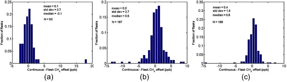
Histograms of the flight differences between continuous (CRDS) and flask measurements of CO2 (Fig. 9), CH4 (Fig. 10) and CO (Fig. 11) show little bias but significant scatter around the mean. Some of the scatter can be attributed to uncertainties in timing; because there is no pressure mea-surement in the flasks, the flask flushing and filling sequence is modeled based on laboratory measurements (Neff, 2013). Some of the scatter, however, cannot be attributed to tim-ing issues. For example, when flasks filled durtim-ing periods of high variability are omitted from the calculation, the standard deviation of offsets is still relatively large compared to the mean. In 2011, the offsets (in situ – flask) for CO2(Fig. 9c) are−0.16 (mean)±0.42 (1-σ )ppm. Considering only flasks filled during periods of low atmospheric variability (1-σ vari-ability in the continuous analyzer over the flask flush and fill time<0.2 ppm), the offsets are−0.20 (mean)±0.27 (1-σ )ppm for CO2. For CH4, the offsets in 2011 change from 0.4±1.8 ppb to 0.4±1.3 ppb when considering flasks filled during variability <3 ppb, and for CO there is no measur-able improvement (from−0.6±2.8 ppb to−0.6±2.6) when considering variability<5 ppb.
The absolute bias (mean) of the CO2, CH4, and CO in situ to flask comparisons is smaller than the variability (1-σ stan-dard deviation) but larger than the stanstan-dard error (σ/
Fig. 9. Differences between continuous (CRDS) CO2measurements and flask CO2measurements during flights over Alaska on the USCG C-130 for three seasons: (a) 2009, (b) 2010, and (c) 2011. Negative offsets occur when the flask-measured mole fraction is higher than the continuous measurement. The mean for each season, 1-σ standard deviation, and number of flasks for comparison are indicated on each figure.
Fig. 10. Differences between continuous (CRDS) CH4measurements and flask CH4 measurements during flights over Alaska on the USCG C-130 for three seasons: (a) 2009, (b) 2010, and (c) 2011. The mean for each season, 1-σ standard deviation, and number of flasks for comparison are indicated on each figure.
in situ comparisons at NOAA ground sites as well, and seem to have become more prevalent since 2011 (Andrews et al., 2013). Laboratory tests are currently underway to determine the cause of these high CO2flask anomalies, which is cur-rently unknown. CO measurements show a mean bias smaller than the WMO compatibility goal (2 ppb) in 2011, and the offsets between the CRDS measurements and the flask mea-surements have been shown to have no dependence on day of year, water vapor, ambient pressure, CO2, CH4, or CO (Chen et al., 2012a).
In 2009, although the scatter of the offsets is small, the me-dian CO2offset is significantly greater than WMO compat-ibility goal (+0.22 ppm). Subsequent re-analysis of the con-tinuous data using only a laboratory calibration from Decem-ber 2009 (i.e., not using the correction of the on-board tanks) reduces the bias to 0.04 ppm. Although we have no reason to reject the in situ calibrations outright, this fact does sug-gest the possibility of a problem in the standard delivery (the tanks were calibrated at NOAA post-mission and were within 0.1 ppm of CO2from their initial calibration, so tank drift is
Fig. 11. Differences between continuous (CRDS) CO measure-ments and flask CO measuremeasure-ments during flights over Alaska on the USCG C-130 for 2011. The mean, 1-σstandard deviation, and number of flasks (N) are indicated on the figure.
The in situ to flask comparison for CO2for all years does not meet the WMO-recommended compatibility of measure-ments (mean of 0.1 ppm for CO2)even when periods of high variability have been filtered out. In trying to understand the cause of this poor repeatability between continuous and flask measurements of CO2, it is important to consider Figs. 6, 7, and 8, which demonstrate the stability of the standard mea-surements not only over a season but also for each flight (standard deviations for both under 0.04 ppm in CO2). Sepa-rate water vapor correction tests suggest that in 1 % water va-por there is an additional uncertainty due to possible drift in the correction of less than 0.1 ppm (Rella et al., 2012). Taken together (∼0.14 ppm when summed in quadrature) these er-rors are significantly smaller than the observed repeatability suggesting that there are errors in gas handling upstream of the standard tank introduction or that there are errors in the flask measurements contributing to poor reproducibility.
To test the integrity of the in situ gas handling, thorough leak checks on all inlet lines are performed whenever possi-ble (prior to each season at the minimum). Two additional tests are performed annually on the aircraft system: (1) a standard gas is run through a portion of the inlet line at am-bient external pressure during flight (by utilizing a tee fitting for excess flow outside the aircraft); and (2) on the ground, a standard gas is run through the complete inlet line from the exterior of the aircraft. These tests are performed at least once per year to evaluate the effects of both low pressure and of any kind of contamination in the inlet line, and have proven valuable in confirming that the in situ analyzer stream has not been contaminated prior to entering the MPV.
Testing of the PFP sampling system is also routinely performed. Laboratory tests done with PFP flasks filled
sequentially with a single tank and compared with sin-gle glass flasks (typically used in the NOAA ground net-work) show measurement offsets of −0.09±0.05 ppm for CO2 (http://www.esrl.noaa.gov/gmd/ccgg/aircraft/qc.html). Recent analysis of wet samples in the laboratory and compar-isons with in situ CO2measurement systems on towers (An-drews et al., 2013) suggest that the PFP flasks may have un-certainties as high as 1 ppm for CO2due to possible surface– water interactions when sampling wet air (as is done on the C-130) or due to residual water vapor in PFP flasks from insufficient drying prior to sampling. Unlike lower-pressure network flasks, the PFP flasks store air samples at 2700 hPa; effects of off-gassing from any surface area exposed to the sample will therefore be amplified. Tests of the PFP flasks and sampling system are on-going at NOAA and are targeted towards both resolving the discrepancy between the in situ and flask measurements and determining a more accurate un-certainty on the flask measurements of CO, CH4, and CO2.
The higher than desired uncertainty for CO2on both sys-tems is a critical reminder that accurate GHG measurements must be validated whenever possible, and that frequent sam-pling of standards during flight may not be an adequate as-sessment of the true uncertainty of a system. When measure-ments are performed autonomously, especially when inde-pendent validation is not routine (e.g., flask vs. in situ com-parisons are not possible), we recommend periodic confir-mation of measurements by either independent validation or rigorous tests such as those described above.
2.6 Water vapor measurement
Fig. 12. Altitude profiles of water vapor (H2O) measurements over Galena on 28 June 2012. Left panel: ascent and descent measure-ments from the CRDS analyzer (data gaps exist during calibra-tion periods). Right panel: ascent measurements from both CRDS (blue) and calculated from in situ temperature and RH measure-ments (red).
the Vaisala temperature and relative humidity measurements, along with the external ambient pressure measurement, and equations from Goff (1957) and Buck (1981). Vertical gradi-ents in H2O are well resolved in both cases, although some difference in response time is apparent (the Vaisala probe has a response time that depends on various factors, including airspeed and the orientation of the protective shield).
Over the 2011 season, measurements from the CRDS analyzer and the T/RH sensor compare well considering the uncertainty in the Vaisala temperature and relative hu-midity measurements is reported to be 1 % of the reading, with a high correlation (R2=0.99) and slope close to unity (Fig. 13). Further analysis, along with laboratory calibration, is required to evaluate the stability and the site-to-site com-parability of the CRDS system for water vapor. However, the flight data show that the CRDS analyzer is capable of captur-ing gradients in H2O that can be used to determine boundary layer height.
3 Results and conclusions
The GHG measurement system designed to operate on the USCG C-130 aircraft in Alaska is simple and robust. We recognize some trade-offs are necessary and have chosen a simple system despite somewhat degraded response time (re-sulting from a slow change in baseline related to water va-por), leading to a loss of some measurements surrounding calibration cycles. The decisions made in favor of a sim-pler system, such as not drying the sample stream, do not increase the measurement error of the in situ data beyond the stated uncertainties, and allow for the measurement of wa-ter vapor. For the 2011 season, estimated uncertainties (of the native 2.5-s measurements) are 0.15 ppm, 1.4 ppb, and 5 ppb for CO2, CH4, and CO respectively, considering short-term precision, calibration uncertainties and water vapor cor-rection uncertainties. In 2009 and 2010, the uncertainties are slightly larger because of inferior short-term precision of the older analyzers: 0.23 ppm (CO2)and 2.3 ppb (CH4).
Fig. 13. Comparison of CRDS H2O with values calculated from the temperature and relative humidity sensor over the entire 2011 season. Red line shows the linear fit to the data, while the black dashed line indicates the 1 : 1 relationship.
Uncertainties are lower for measurements made in low tur-bulence (and therefore better short-term precision than the upper limit we have used in our uncertainty estimate), be-cause the short-term precision contributes significantly to the total uncertainty. From 2012 onward, we expect lower un-certainties for CO2and CH4than 2011 because of the better pressure control of the analyzer cell after the installation of a new proportional valve (Sect. 2.2.3). These results do not suggest that variations in pressure or temperature affect the CRDS measurements in any way.
The large size of the aircraft used at this site allows for a relatively large payload, which has allowed NOAA to de-ploy flasks along with the CRDS system for measuring CO2, CH4, and CO, thus giving a real assessment of the uncertain-ties for each. The C-130 payload capacity also allows for the deployment of three gas standard tanks for calibration of the CRDS analyzer, allowing us to evaluate the optimal in-flight calibration strategy. We have found that high frequency (ev-ery 30 min) calibrations may not be necessary because of the high stability of the CRDS analyzer. For ACG flights, the same low measurement error could be achieved by running two reference tanks at a frequency that allows for at least two measurements of each tank during a single flight (to confirm repeatability), for example at the start and end of each flight. Deploying only a single tank would be acceptable but would make it more difficult to assess degradation in the tank itself as a cause of drift in the measurement.
both the standards and the sample. In the case of our ACG de-ployments, it would have been possible to deploy our anal-ysis system without standards given the low flight-to-flight variability of the laboratory calibration with respect to in-flight measurements. However, we recommend that a target gas be used to track drift between flights if possible. It is worth noting that the most significant measurement prob-lem encountered to date was the depletion of CO2 in the aluminum inlet line early in the 2011 season. This problem could not have been discovered based on in-flight calibra-tions and was revealed only by comparison with independent flask measurements. Periodic tests, as frequently as possi-ble, of the entire system inlet are also recommended. Over-all, three years of autonomous aircraft deployment of the CRDS system suggest that six-month deployments are pos-sible without on-board calibrations, provided rigorous pre-and post-deployment laboratory tests are performed, includ-ing checkinclud-ing sample handlinclud-ing, water vapor testinclud-ing, and quan-tifying drift from standards calibrated on the WMO scale. The expected uncertainty of such measurements without on-board calibrations (using the current ACG analyzer unit with a new proportional valve with better pressure control) is 0.13 ppm for CO2, 1.4 ppb for CH4, and 5 ppb for CO, essen-tially the same as the estimated uncertainty of our 2011 mea-surements with on-board calibrations but without the new valve.
Data acquired at the Alaska Coast Guard site over three seasons have been shown to be of high quality and will be valuable for investigations of the Arctic and boreal carbon cycle. These repeated measurements from the same locations in different seasons and years are valuable for determining seasonal and long-term trends as well as inter-annual vari-ability. Data from ACG are available from the corresponding author until they become available online at the NOAA Car-bon Cycle server (http://www.esrl.noaa.gov/gmd/dv/data/).
Acknowledgements. We would like to acknowledge the valuable assistance of Jason Manthey, our current technician and operator in Kodiak, Alaska, our past technician, Margo Connolly, and the US Coast Guard Air Station Kodiak. We would also like to acknowl-edge the extensive help we have received from Doug Guenther, Jack Higgs, Paul Novelli, Pat Lang, Ed Dlugokencky, Du-ane Kitzis, Laura Patrick, Sam Oltmans, and Sara Crepinsek, all at NOAA/ESRL Global Monitoring Division. We thank Chris Rella at Picarro for valuable assistance with various aspects of the CRDS gas analyzers, and the CARVE Science Team for assistance and advice. This effort was funded by NOAA through the North American Carbon Program.
Edited by: O. Tarasova
References
Andrews, A. E., Kofler, J. D., Trudeau, M. E., Williams, J. C., Neff, D. H., Masarie, K. A., Chao, D. Y., Kitzis, D. R., Novelli, P. C., Zhao, C. L., Dlugokencky, E. J., Lang, P. M., Crotwell, M. J., Fischer, M. L., Parker, M. J., Lee, J. T., Baumann, D. D., Desai, A. R., Stanier, C. O., de Wekker, S. F. J., Wolfe, D. E., Munger, J. W., and Tans, P. P.: CO2, CO and CH4 mea-surements from the NOAA Earth System Research Laboratory’s Tall Tower Greenhouse Gas Observing Network: instrumenta-tion, uncertainty analysis and recommendations for future high-accuracy greenhouse gas monitoring efforts, Atmos. Meas. Tech. Discuss., 6, 1461–1553, doi:10.5194/amtd-6-1461-2013, 2013. Biraud, S. C., Torn, M. S., Smith, J. R., Sweeney, C., Riley, W. J.,
and Tans, P. P.: A multi-year record of airborne CO2observations in the US Southern Great Plains, Atmos. Meas. Tech. Discuss., 5, 7187–7222, doi:10.5194/amtd-5-7187-2012, 2012.
Buck, A. L.: New Equations for Computing Vapor Pressure and Enhancement Factor, J. Appl. Meteorol., 20, 1527–1532, doi:10.1175/1520-0450(1981)020<1527:NEFCVP>2.0.CO;2, 1981.
Cambaliza, M. O. L., Shepson, P., Stirm, B., Sweeney, C., Turn-bull, J., Karion, A., Davis, K., Lauvaux, T., Richardson, S., Miles, N., and Svetanoff, R.: Quantification of emissions from methane sources in Indianapolis using an aircraft-based platform, Abstr. Pap. Am. Chem. S., Publ. No.‘473, 2011.
Chen, H., Winderlich, J., Gerbig, C., Hoefer, A., Rella, C. W., Crosson, E. R., Van Pelt, A. D., Steinbach, J., Kolle, O., Beck, V., Daube, B. C., Gottlieb, E. W., Chow, V. Y., Santoni, G. W., and Wofsy, S. C.: High-accuracy continuous airborne measure-ments of greenhouse gases (CO2and CH4) using the cavity ring-down spectroscopy (CRDS) technique, Atmos. Meas. Tech., 3, 375–386, doi:10.5194/amt-3-375-2010, 2010.
Chen, H., Karion, A., Rella, C. W., Winderlich, J., Gerbig, C., Filges, A., Newberger, T., Sweeney, C., and Tans, P. P.: Accurate measurements of carbon monoxide in humid air using the cavity ring-down spectroscopy (CRDS) technique, Atmos. Meas. Tech. Discuss., 5, 6493–6517, doi:10.5194/amtd-5-6493-2012, 2012a. Chen, H., Winderlich, J., Gerbig, C., Katrynski, K., Jordan, A., and Heimann, M.: Validation of routine continuous airborne CO2 ob-servations near the Bialystok Tall Tower, Atmos. Meas. Tech., 5, 873–889, doi:10.5194/amt-5-873-2012, 2012b.
Conway, T. J., Steele, L. P., and Novelli, P. C.: Correlations among atmospheric CO2, CH4and CO in the Arctic, March 1989, At-mos. Environ. A-Gen., 27, 2881–2894, 1993.
Crosson, E. R.: A cavity ring-down analyzer for measuring atmo-spheric levels of methane, carbon dioxide, and water vapor, Appl. Phys. B-Lasers O., 92, 403–408, doi:10.1007/s00340-008-3135-y, 2008.
Daube, B. C., Boering, K. A., Andrews, A. E., and Wofsy, S. C.: A high-precision fast-response airborne CO2analyzer for in situ sampling from the surface to the middle stratosphere, J. Atmos. Ocean. Tech., 19, 1532–1543, 2002.
Forster, P., Ramaswamy, V., Artaxo, P., Berntsen, T., Betts, R., Fa-hey, D. W., and Haywood, J.: Changes in Atmospheric Con-stituents and in Radiative Forcing, in: Climate Change 2007: The Physical Science Basis, Contribution of Working Group I to the Fourth Assessment Report of the IPCC, edited by: Solomon, S., Qin, D., Manning, M., Chen, Z., Marquis, M., Averyt, K. B., Tig-nor, M., and Miller, H. L., Cambridge University Press, Cam-bridge, United Kingdom and New York, NY, USA, 2007. Goff, J. A.: Saturation pressure of water on the new Kelvin
temper-ature scale, Transactions of the American Society of Heating and Ventilating Engineers, Murray Bay, Quebec, Canada, 1957. Hall, B. D., Dutton, G. S., and Elkins, J. W.: The NOAA nitrous
oxide standard scale for atmospheric observations, J. Geophys. Res., 112, doi:10.1029/2006jd007954, 2007.
Harriss, R. C., Sachse, G. W., Hill, G. F., Wade, L., Bartlett, K. B., Collins, J. E., Steele, L. P., and Novelli, P. C.: Carbon-monoxide and methane in the North-American Arctic and sub-Arctic tro-posphere – July–August 1988, J. Geophys. Res.-Atmos., 97, 16589–16599, 1992.
Harriss, R. C., Sachse, G. W., Collins, J. E., Wade, L., Bartlett, K. B., Talbot, R. W., Browell, E. V., Barrie, L. A., Hill, G. F., and Burney, L. G.: Carbon-monoxide and methane over Canada – July–August 1990, J. Geophys. Res.-Atmos., 99, 1659–1669, 1994.
Jacob, D. J., Crawford, J. H., Maring, H., Clarke, A. D., Dibb, J. E., Emmons, L. K., Ferrare, R. A., Hostetler, C. A., Russell, P. B., Singh, H. B., Thompson, A. M., Shaw, G. E., McCauley, E., Ped-erson, J. R., and Fisher, J. A.: The Arctic Research of the Compo-sition of the Troposphere from Aircraft and Satellites (ARCTAS) mission: design, execution, and first results, Atmos. Chem. Phys., 10, 5191–5212, doi:10.5194/acp-10-5191-2010, 2010.
Jorgenson, M. T., Racine, C. H., Walters, J. C., and Osterkamp, T. E.: Permafrost degradation and ecological changes associated with a warming climate in central Alaska, Climatic Change, 48, 551–579, 2001.
Keyser, A. R., Kimball, J. S., Nemani, R. R., and Running, S. W.: Simulating the effects of climate change on the carbon balance of North American high-latitude forests, Glob. Change Biol., 6, 185–195, 2000.
Kort, E. A., Wofsy, S. C., Daube, B. C., Diao, M., Elkins, J. W., Gao, R. S., Hintsa, E. J., Hurst, D. F., Jimenez, R., Moore, F. L., Spackman, J. R., and Zondlo, M. A.: Atmospheric observations of Arctic Ocean methane emissions up to 82 degrees north, Nat. Geosci., 5, 318–321, doi:10.1038/ngeo1452, 2012.
Machida, T., Matsueda, H., Sawa, Y., Nakagawa, Y., Hirotani, K., Kondo, N., Goto, K., Nakazawa, T., Ishikawa, K., and Ogawa, T.: Worldwide Measurements of Atmospheric CO2and Other Trace Gas Species Using Commercial Airlines, J. Atmos. Ocean. Tech., 25, 1744–1754, doi:10.1175/2008jtecha1082.1, 2008.
Martins, D. K., Sweeney, C., Stirm, B. H., and Shepson, P. B.: Re-gional surface flux of CO2inferred from changes in the advected CO2 column density, Agr. Forest Meteorol., 149, 1674–1685, doi:10.1016/j.agrformet.2009.05.005, 2009.
Mays, K. L., Shepson, P. B., Stirm, B. H., Karion, A., Sweeney, C., and Gurney, K. R.: Aircraft-based measurements of the carbon footprint of Indianapolis, Environ. Sci. Technol., 43, 7816–7823, doi:10.1021/es901326b, 2009.
McGuire, A. D., Anderson, L. G., Christensen, T. R., Dallimore, S., Guo, L. D., Hayes, D. J., Heimann, M., Lorenson, T. D.,
Mac-donald, R. W., and Roulet, N.: Sensitivity of the carbon cycle in the Arctic to climate change, Ecol. Monogr., 79, 523–555, 2009. Miles, N. L., Richardson, S. J., Davis, K. J., Lauvaux, T., An-drews, A. E., West, T. O., Bandaru, V., and Crosson, E. R.: Large amplitude spatial and temporal gradients in atmospheric bound-ary layer CO2mole fractions detected with a tower-based net-work in the US upper Midwest, J. Geophys. Res., 117, G01019, doi:10.1029/2011jg001781, 2012.
Miller, J. B., Gatti, L. V., d’Amelio, M. T. S., Crotwell, A. M., Dlugokencky, E. J., Bakwin, P., Artaxo, P., and Tans, P. P.: Airborne measurements indicate large methane emissions from the eastern Amazon basin, Geophys. Res. Lett., 34, L10809, doi:10.1029/2006gl029213, 2007.
Montzka, S. A., Myers, R. C., Butler, J. H., Elkins, J. W., and Cum-mings, S. O.: Global tropospheric distribution and calibration scale of HCFC-22, Geophys. Res. Lett., 20, 703–706, 1993. Nara, H., Tanimoto, H., Tohjima, Y., Mukai, H., Nojiri, Y.,
Katsumata, K., and Rella, C. W.: Effect of air composition (N2, O2, Ar, and H2O) on CO2 and CH4 measurement by wavelength-scanned cavity ring-down spectroscopy: calibration and measurement strategy, Atmos. Meas. Tech., 5, 2689–2701, doi:10.5194/amt-5-2689-2012, 2012.
Neff, D.: The Programmable Flask Package Air Sampling System, in preparation, 2013.
Novelli, P. C.: Reanalysis of tropospheric CO trends: Effects of the 1997–1998 wildfires, J. Geophys. Res., 108, 13109–13121, doi:10.1029/2002jd003031, 2003.
Novelli, P. C., Elkins, J. W., and Steele, L. P.: The development and evaluation of a gravimetric reference scale for measurements of atmospheric carbon monoxide, J. Geophys. Res.-Atmos., 96, 13109–13121, doi:10.1029/91jd01108, 1991.
O’Connor, F. M., Boucher, O., Gedney, N., Jones, C. D., Folberth, G. A., Coppell, R., Friedlingstein, P., Collins, W. J., Chappel-laz, J., Ridley, J., and Johnson, C. E.: Possible role of wetlands, permafrost, and methane hydrates in the methane cycle under future climate change: A review, Rev. Geophys., 48, RG4005, doi:10.1029/2010rg000326, 2010.
O’Shea, S. J., Bauguitte, S. J.-B., Gallagher, M. W., Lowry, D., and Percival, C. J.: Development of a cavity enhanced absorption spectrometer for airborne measurements of CH4and CO2, At-mos. Meas. Tech. Discuss., 6, 1–41, doi:10.5194/amtd-6-1-2013, 2013.
Paris, J. D., Ciais, P., Nedelec, P., Ramonet, M., Belan, B. D., Ar-shinov, M. Y., Golitsyn, G. S., Granberg, I., Stohl, A., Cayez, G., Athier, G., Boumard, F., and Cousin, J. M.: The YAK-AEROSIB transcontinental aircraft campaigns: new insights on the trans-port of CO2, CO and O-3 across Siberia, Tellus B, 60, 551–568, doi:10.1111/j.1600-0889.2008.00369.x, 2008.
Rella, C. W., Chen, H., Andrews, A. E., Filges, A., Gerbig, C., Hatakka, J., Karion, A., Miles, N. L., Richardson, S. J., Stein-bacher, M., Sweeney, C., Wastine, B., and Zellweger, C.: High accuracy measurements of dry mole fractions of carbon diox-ide and methane in humid air, Atmos. Meas. Tech. Discuss., 5, 5823–5888, doi:10.5194/amtd-5-5823-2012, 2012.
Sweeney, C., Karion, A., Wolter, S., Neff, D., Higgs, J. A., Heller, M., Guenther, D., Miller, B. R., Montzka, S. A., Miller, J. B., Conway, T. J., Dlugokencky, E., Novelli, P. C., Masarie, K., Oltman, S., and Tans, P.: Carbon dioxide climatology of the NOAA/ESRL Greenhouse Gas Aircraft Network, in preparation, 2013.
Turnbull, J. C., Karion, A., Fischer, M. L., Faloona, I., Guilder-son, T., Lehman, S. J., Miller, B. R., Miller, J. B., Montzka, S., Sherwood, T., Saripalli, S., Sweeney, C., and Tans, P. P.: Assess-ment of fossil fuel carbon dioxide and other anthropogenic trace gas emissions from airborne measurements over Sacramento, California in spring 2009, Atmos. Chem. Phys., 11, 705–721, doi:10.5194/acp-11-705-2011, 2011.
Vaughn, B. H., Ferretti, D. F., Miller, J. B., and White, J. W. C.: Stable isotope measurements of atmospheric CO2and CH4, in: Handbook of stable isotope analytical techniques, Elsevier BV, Amsterdam, The Netherlands, 2004.
Vay, S. A., Choi, Y., Vadrevu, K. P., Blake, D. R., Tyler, S. C., Wisthaler, A., Hecobian, A., Kondo, Y., Diskin, G. S., Sachse, G. W., Woo, J. H., Weinheimer, A. J., Burkhart, J. F., Stohl, A., and Wennberg, P. O.: Patterns of CO2 and radiocarbon across high northern latitudes during International Polar Year 2008, J. Geophys. Res., 116, D14301, doi:10.1029/2011jd015643, 2011.
Winderlich, J., Chen, H., Gerbig, C., Seifert, T., Kolle, O., Lavriˇc, J. V., Kaiser, C., H¨ofer, A., and Heimann, M.: Continuous low-maintenance CO2/CH4/H2O measurements at the Zotino Tall Tower Observatory (ZOTTO) in Central Siberia, Atmos. Meas. Tech., 3, 1113–1128, doi:10.5194/amt-3-1113-2010, 2010. Wofsy, S. C., Team, H. S., Cooperating Modellers, T., and
Satel-lite, T.: HIAPER Pole-to-Pole Observations (HIPPO): fine-grained, global-scale measurements of climatically important at-mospheric gases and aerosols, Philos. T. Roy. Soc. A, 369, 2073– 2086, doi:10.1098/rsta.2010.0313, 2011.
Xueref-Remy, I., Messager, C., Filippi, D., Pastel, M., Nedelec, P., Ramonet, M., Paris, J. D., and Ciais, P.: Variability and budget of CO2in Europe: analysis of the CAATER airborne campaigns – Part 1: Observed variability, Atmos. Chem. Phys., 11, 5655– 5672, doi:10.5194/acp-11-5655-2011, 2011.