www.atmos-meas-tech.net/8/2961/2015/ doi:10.5194/amt-8-2961-2015
© Author(s) 2015. CC Attribution 3.0 License.
Consistent satellite XCO
2
retrievals from SCIAMACHY and
GOSAT using the BESD algorithm
J. Heymann1, M. Reuter1, M. Hilker1, M. Buchwitz1, O. Schneising1, H. Bovensmann1, J. P. Burrows1, A. Kuze2, H. Suto2, N. M. Deutscher1,4, M. K. Dubey3, D. W. T. Griffith4, F. Hase5, S. Kawakami2, R. Kivi6, I. Morino7, C. Petri1, C. Roehl8, M. Schneider5, V. Sherlock9,a, R. Sussmann10, V. A. Velazco4, T. Warneke1, and D. Wunch8 1Institute of Environmental Physics (IUP), University of Bremen, Bremen, Germany
2Japan Aerospace Exploration Agency (JAXA), Tsukuba, Japan 3Los Alamos National Laboratory, Los Alamos, USA
4Centre for Atmospheric Chemistry, University of Wollongong, Wollongong, Australia 5IMK-ASF, Karlsruhe Institute of Technology (KIT), Karlsruhe, Germany
6Finnish Meteorological Institute, Sodankylä, Finland
7National Institute for Environmental Studies (NIES), Tsukuba, Japan 8California Institute of Technology, Pasadena, USA
9National Institute of Water and Atmospheric Research, Wellington, New Zealand 10IMK-IFU, Karlsruhe Institute of Technology (KIT), Garmisch-Partenkirchen, Germany anow at: Laboratoire de Météorologie Dynamique, Palaiseau, France
Correspondence to: J. Heymann ([email protected])
Received: 19 December 2014 – Published in Atmos. Meas. Tech. Discuss.: 13 February 2015 Revised: 22 June 2015 – Accepted: 4 July 2015 – Published: 24 July 2015
Abstract. Consistent and accurate long-term data sets of global atmospheric concentrations of carbon dioxide (CO2) are required for carbon cycle and climate-related research. However, global data sets based on satellite observations may suffer from inconsistencies originating from the use of products derived from different satellites as needed to cover a long enough time period. One reason for inconsis-tencies can be the use of different retrieval algorithms. We address this potential issue by applying the same algorithm, the Bremen Optimal Estimation DOAS (BESD) algorithm, to different satellite instruments, SCIAMACHY on-board ENVISAT (March 2002–April 2012) and TANSO-FTS on-board GOSAT (launched in January 2009), to retrieve XCO2, the column-averaged dry-air mole fraction of CO2. BESD has been initially developed for SCIAMACHY XCO2 re-trievals. Here, we present the first detailed assessment of the new GOSAT BESD XCO2product. GOSAT BESD XCO2is a product generated and delivered to the MACC project for assimilation into ECMWF’s Integrated Forecasting System. We describe the modifications of the BESD algorithm needed in order to retrieve XCO2 from GOSAT and present
missions (e.g. OCO-2, GOSAT-2, CarbonSat) in the future.
1 Introduction
Space-based observations of carbon dioxide (CO2) can con-tribute to the elimination of important knowledge gaps re-lated to the regional sources and sinks of CO2(Rayner and O’Brien, 2001; Hungershoefer et al., 2010; Schneising et al., 2013, 2014; Reuter et al., 2014b, c). Near-surface sensitive measurements of column-averaged dry-air mole fractions of CO2 (XCO2) in the short-wave infrared spectral region (SWIR) are well suited for this application. These observa-tions can complement measurements from existing surface-based greenhouse gas monitoring networks, especially in data-poor regions, by providing data with dense spatial cov-erage. However, satellite measurements need to be precise and accurate enough to reduce uncertainties in the character-isation of the sources and sinks. Studies showed that a pre-cision of better than 1 % for regional averages and monthly means (Rayner and O’Brien, 2001; Houweling et al., 2004) and regional biases of less than a few tenth of a part per mil-lion (ppm) are required (Chevallier et al., 2007; Miller et al., 2007).
The SCanning Imaging Absorption spectroMeter for At-mospheric CHartographY (SCIAMACHY) on-board the Eu-ropean Space Agency’s (ESA) Environmental Satellite (EN-VISAT) (Burrows et al., 1995; Bovensmann et al., 1999), launched in 2002, was in the time period before mid-2009 the only satellite instrument measuring XCO2 with high surface sensitivity. The long-term time series of surface-sensitive satellite-derived XCO2 starts with SCIAMACHY. SCIAMACHY had observed the Earth’s atmosphere until the loss of ENVISAT in April 2012.
The Thermal And Near infrared Sensor for carbon Obser-vations Fourier Transform Spectrometer (TANSO-FTS) on-board the Greenhouse gases Observing SATellite (GOSAT) (Kuze et al., 2009), launched in January 2009, and the Or-biting Carbon Observatory-2 (OCO-2) (Crisp et al., 2004), launched in July 2014, are currently the only satellite in-struments yielding XCO2with high near-surface sensitivity. Both satellite missions are specifically designed to observe XCO2.
Several retrieval algorithms have been developed to evaluate the satellite observations for SCIAMACHY (e.g. Schneising et al., 2012; Heymann et al., 2012b; Reuter et al., 2011) and for GOSAT (e.g. Yoshida et al., 2013; Crisp et al., 2012; Guerlet et al., 2013; Cogan et al., 2012; Oshchep-kov et al., 2008). These algorithms differ e.g. in cloud and aerosol treatment, state vector elements and cloud filtering (for more details see, e.g. Reuter et al., 2013; Takagi et al., 2014). One of these algorithms is the Bremen Optimal Esti-mation DOAS (BESD) retrieval algorithm developed for the
of Bremen (Reuter et al., 2010, 2011). As unaccounted scat-tering by aerosols and clouds is a major error source for satel-lite retrievals (e.g. Aben et al., 2006; Houweling et al., 2005; Heymann et al., 2012a; Guerlet et al., 2013), BESD aims to reduce this error source by explicitly considering atmo-spheric scattering (Reuter et al., 2010). The BESD algorithm has been used to generate a SCIAMACHY XCO2data prod-uct ranging from 2002 to 2012. This data prodprod-uct has been used in several key European projects, e.g. ESA’s Climate Change Initiative (CCI, www.esa-ghg-cci.org and Buchwitz et al., 2013b; Hollmann et al., 2013) and the EU’s Mon-itoring of Atmospheric Composition and Climate (MACC, Hollingsworth et al., 2008) project.
Carbon cycle and climate-related research requires consis-tent and accurate long-term global CO2data sets. However, global data sets based on observations from different satel-lite instruments may suffer from inconsistencies originating from the use of different satellite algorithms. We address this potential issue by applying the same retrieval algorithm, the BESD algorithm, to different satellite instruments, SCIA-MACHY and TANSO-FTS. Within the European MACC project, after the loss of ENVISAT, the BESD algorithm has been modified to also retrieve XCO2from TANSO-FTS mea-surements. The GOSAT/TANSO-FTS BESD XCO2product was delivered for the assimilation into the European Centre for Medium-range Weather Forecasts (ECMWF) Integrated Forecasting System (Agustí-Panareda et al., 2014). Here, we report first results of an assessment of the new GOSAT BESD XCO2 data product. In addition, we discuss results of an investigation concerning the consistency of the SCIA-MACHY BESD and GOSAT BESD XCO2 data sets. This analysis includes a comparison of validation results obtained by using data from the Total Carbon Column Observing Net-work (TCCON, Wunch et al., 2011a), a direct comparison of daily satellite-based XCO2data and a global comparison with NOAA’s CO2modelling and assimilation system Car-bonTracker (Peters et al., 2007).
2 SCIAMACHY on ENVISAT
The satellite instrument SCIAMACHY (Burrows et al., 1995; Bovensmann et al., 1999) was part of the atmo-spheric chemistry payload on-board ESA’s ENVISAT. The ENVISAT satellite was launched in March 2002. On 8 April 2012, after 10 years of operation, ESA lost contact to VISAT and finally had declared the official end of the EN-VISAT mission on 9 May 2012. ENEN-VISAT flew on a sun-synchronous daytime (descending) orbit with an equator crossing time of 10:00 local time (LT).
The SCIAMACHY instrument was a passive remote sens-ing moderate-resolution imagsens-ing spectrometer and measured sunlight transmitted, reflected and scattered by the Earth’s atmosphere or surface in the ultraviolet, visible and near-infrared wavelength regions in eight spectral channels (214– 1750, 1940–2040, 2265–2380 nm) with a spectral resolution between 0.2 and 1.4 nm. The scientific objective of SCIA-MACHY was to improve our knowledge of global atmo-spheric change and related issues of importance to the chem-istry and physics of the atmosphere, i.e. the impact of pollu-tion, exchange processes between atmospheric layers, atmo-spheric chemistry in polar and other regions and the influence of natural phenomena such as volcanic eruptions. Targets of SCIAMACHY were atmospheric gases (e.g. O3, NO2, CH4 and CO2) as well as clouds and aerosols, ocean colour and land parameters. SCIAMACHY measured in three different viewing geometries: nadir, limb and solar/lunar occultation.
For the work presented in this study the nadir mode ob-servations in channel 4 (755–775 nm) and channel 6 (1558– 1594 nm) has been used. The integration time of the instru-ment in the used spectral regions was typically 0.25 s. This provided a typical spatial resolution of∼60 km across track and ∼30 km along track. By scanning ±32◦ across track, SCIAMACHY achieved a swath width of∼1000 km.
3 TANSO-FTS on GOSAT
GOSAT was the first satellite mission dedicated to mea-suring atmospheric XCO2 and XCH4 (Kuze et al., 2009). GOSAT is a joint project of the Japanese Aerospace Explo-ration Agency, the National Institute for Environmental Stud-ies and the Ministry of the Environment. The objectives of GOSAT are to monitor the global distribution of greenhouse gases, to estimate CO2and CH4sources and sinks on sub-continental scale and to verify reductions of anthropogenic greenhouse gas emissions (Kuze et al., 2009). On 23 January 2009, GOSAT was launched in a sun-synchronous daytime orbit with an equator crossing time of 13:00 (LT).
GOSAT carries two satellite instruments, the TANSO-FTS and the Cloud and Aerosol Imager (TANSO-CAI). The TANSO-FTS is a double pendulum interferometer. It mea-sures two orthogonal polarisation directions of reflected or scattered sunlight in three bands (bands 1, 2, 3) in the SWIR
between 4800 and 13 200 cm−1(758–2083 nm). In addition to the SWIR bands, band 4 measures in the thermal in-frared between 700 and 1800 cm−1 (5.56–14.3 µm). How-ever, measurements obtained with band 4 are not consid-ered in this paper. TANSO-FTS has a spectral resolution of 1ν1≈0.36 cm−1(1λ1≈0.02 nm) in band 1 and1ν2,3≈ 0.26 cm−1(1λ2≈0.07 and1λ3≈0.1 nm) in bands 2 and 3. In order to improve the dynamic range of the instrument, the scientific measurements of TANSO-FTS are performed in two gain modes, medium (M) and high (H), used accord-ing to the measured level of intensity. For example, gain M is used over bright surfaces such as deserts. With an in-stantaneous field of view (IFOV) of 15.8 mrad (∼10.5 km diameter at nadir when projected to the ground), TANSO-FTS can measure±35◦across track and±20◦along track. The typically used scan time of one interferogram is 4 s. Be-tween 4 April 2009 and 31 July 2010, the five-point across track mode was used, which yields footprints separated by ∼158 km across track and∼152 km along track at the equa-tor (e.g. Crisp et al., 2012). In order to improve the pointing stability during the scans, on 1 August 2010 the observation mode was changed to a three-point across track mode with footprints separated by∼263 km across track and∼283 km along track at the equator.
The TANSO-CAI instrument is a high spatial resolution imager detecting clouds and optically thick aerosol layers within the TANSO-FTS field of view. The TANSO-CAI data products are not used for the BESD algorithm.
4 SCIAMACHY BESD algorithm
The BESD retrieval algorithm has been developed at the Uni-versity of Bremen to retrieve XCO2 from SCIAMACHY nadir measurements. BESD aims to minimise scattering-related errors of the retrieved XCO2. For this purpose, the algorithm explicitly accounts for scattering. The theoretical basis of BESD and a study of synthetic retrievals is presented in the publication of Reuter et al. (2010) and validation re-sults are presented in Reuter et al. (2011).
The algorithm is a core algorithm within ESA’s CCI (Holl-mann et al., 2013; Buchwitz et al., 2013b; Dils et al., 2014) aiming at delivering high-quality satellite retrievals. Here we use the most recent product version (02.00.08) of SCIA-MACHY BESD, which is part of the Climate Research Data Package (CRDP#2) of the CCI project. A detailed descrip-tion of the current version of BESD can be found in the Al-gorithm Theoretical Basis Document (ATBD) (Reuter et al., 2014a, available at http://www.esa-ghg-cci.org/). Here, only a short overview of the algorithm is given.
edge. The state vector consists of 26 elements. These ele-ments include a wavelength shift and the full width half max-imum (FWHM) of a Gaussian-shaped instrumental slit func-tion, both fitted separately in the O2 and CO2 fit window. A Lambertian surface albedo with smooth spectral progres-sion expressed as a second-order polynomial (with polyno-mial coefficientsP0,P1 andP2) is fitted separately in both fit windows. A 10-layered CO2 mixing ratio profile, which is separated in equally spaced pressure intervals, is fitted in the CO2 fit window. The correlated a priori errors of the CO2 profile layers provide a degree of freedom of the re-trieved XCO2 of ∼1.0. Reanalysis profiles (ERA-Interim, Dee et al., 2011) of pressure, temperature and humidity pro-vided by the ECMWF are used for the forward model calcu-lation needed to calculate simulated SCIAMACHY spectra. The surface pressure, a shift of the temperature profile and the H2O column-averaged mole fraction are fitted in the O2 and CO2window simultaneously.
Atmospheric scattering is considered by fitting three scattering-related parameters. A thin ice cloud layer consist-ing of fractal ice crystals with 50 µm effective radius and a thickness of 0.5 km is defined for the forward model calcu-lations. Within the retrieval, the cloud water path (CWP) and the cloud top height (CTH) are retrieved. Aerosols are con-sidered by using a standard LOWTRAN summer aerosol pro-file with moderate rural aerosol load. A Henyey–Greenstein phase function is used and the total optical thickness is about 0.136 at 750 nm and 0.038 at 1550 nm. The aerosol retrieval is based on scaling the predefined aerosol profile (aerosol profile scaling (APS) factor). Not only the scattering param-eters but also the paramparam-eters defining the meteorological sit-uation are fitted simultaneously via a merged fit window ap-proach. Simultaneous fitting in both fit windows transfers in-formation, e.g. in case of scattering parameters, mostly ob-tained from the O2-A band to the CO2band.
The forward model is the radiative transfer model SCI-ATRAN (Rozanov et al., 2014). SCISCI-ATRAN calculates the needed radiance spectra and weighting functions, which are the derivatives of the measured radiation. The correlated-k approach of Buchwitz et al. (2000) is used to accelerate the radiative transfer calculations. Line parameters from NASA’s absorption cross section database ABSCO v4.0 (Thompson et al., 2012) is used for O2. The HITRAN 2008 database (Rothman et al., 2009) are used for the other gases. The cal-culated spectra are convolved with a Gaussian slit function.
Although BESD has been designed to minimise scattering-related retrieval errors, clouds are still an important poten-tial error source and strict cloud filtering is necessary. BESD filters clouds by using cloud information based on mea-surements of the Medium Resolution Imaging Spectrometer (MERIS).
The post-processing of the retrieved data includes strict quality filtering and an empirical bias correction. This is needed due to the demanding accuracy requirements on
SCIAMACHY BESD is described in the BESD ATBD (Reuter et al., 2014a).
5 GOSAT BESD algorithm
The GOSAT BESD algorithm is based on the SCIAMACHY BESD algorithm which has been modified to also retrieve XCO2from GOSAT. Here, an overview of the modifications of BESD are given.
5.1 Level 1C data generation
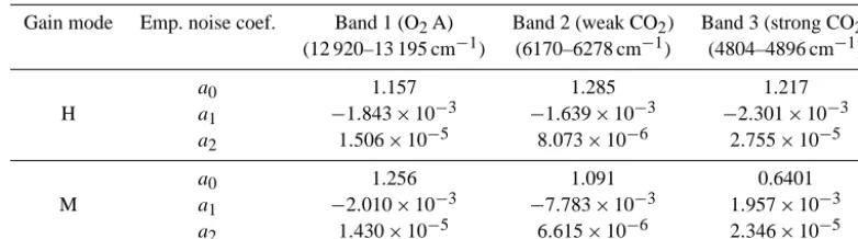
GOSAT BESD uses GOSAT Level 1B data (L1B) ver-sion 161160. These data have been obtained from the GOSAT User Interface Gateway (http://data.gosat.nies.go. jp/GosatUserInterfaceGateway/guig/GuigPage/open.do) and from ESA’s GOSAT Third Party Mission data archive. The (uncalibrated) L1B data have been converted into calibrated Level 1C (L1C) data, by using e.g. the radiance correction scheme described by Yoshida et al. (2012). The L1C data consist of the fully calibrated total intensity, an estimation of the measurement error and a priori information. The to-tal intensity is computed by using the polarisation synthe-sis method described by Yoshida et al. (2011) using the Mueller matrices described by Kuze et al. (2009). The mea-surement noise (εmeas) is estimated by the standard deviation of the first 500 and the last 500 off-band spectral points of GOSAT bands 1, 2 and 3. These spectral points lie outside the band pass filter and can therefore provide a good estimate of εmeas. However, using only the estimate of the measurement noise for the retrieval neglects the contribution of the for-ward model error. Therefore, empirical noise (εempirical) has been implemented and used as described by Yoshida et al. (2013) and Crisp et al. (2012). In order to account for the forward model error, we make the same assumptions as done by Yoshida et al. (2013). We assume that our forward model error increases as the signal-to-noise ratio (SNR) increases. Using the same formula as given by Yoshida et al. (2013),
εempirical=εmeas· q
a0+a1SNR+a2SNR2, (1) and evaluating the relationship between SNR and the mean squared values of the residual spectra delivers the coefficients a0,a1anda2in each spectral window. The coefficients are listed in Table 1.
Table 1. Coefficients for empirical noise for GOSAT high (H) and medium (M) gain observations over land.
Gain mode Emp. noise coef. Band 1 (O2A) Band 2 (weak CO2) Band 3 (strong CO2) (12 920–13 195 cm−1) (6170–6278 cm−1) (4804–4896 cm−1)
a0 1.157 1.285 1.217
H a1 −1.843×10⁻³ −1.639×10⁻³ −2.301×10⁻³ a2 1.506×10⁻⁵ 8.073×10⁻⁶ 2.755×10⁻⁵
a0 1.256 1.091 0.6401
M a1 −2.010×10⁻³ −7.783×10⁻³ 1.957×10⁻³
a2 1.430×10⁻⁵ 6.615×10⁻⁶ 2.346×10⁻⁵
(sun-normalised GOSAT intensity divided by the cosine of the solar zenith angle).
5.2 GOSAT XCO2(Level 2) generation
The GOSAT XCO2 (Level 2) data have been generated by using a modified version of the SCIAMACHY BESD re-trieval algorithm. The main modifications are the follow-ing: we have used three bands instead of two bands (as used for SCIAMACHY) for the retrieval of GOSAT XCO2. Band 1 includes the O2-A band (12 920–13 195 cm−1 or 758–774 nm), band 2 contains a weak CO2absorption band (6170–6278 cm−1 or 1593–1621 nm) and band 3 includes a strong CO2 absorption band (4804–4896 cm−1 or 2042– 2082 nm).
The state vector of GOSAT BESD consists of 38 elements instead of 26 for SCIAMACHY BESD. The state vector ele-ments, their a priori values and uncertainties are listed in Ta-ble 2. A second-order albedo polynomial is additionally fitted in the third fit window. Besides a spectral shift of the nadir radiance, a shift of the solar spectrum is fitted. Instead of the FWHM of a SCIAMACHY Gaussian slit function, param-eters defining the instrumental line shape function (ILS) of TANSO-FTS are fitted. These parameters are the maximum optical path difference (MOPD) and the IFOV. The ILS is calculated (similar as done by e.g. Reuter et al., 2012a) from
ILS(ν)∝5
8ν
ν0IFOV
⊗sinc(2ν·MOPD). (2)
Here,νis the wavenumber (centred around 0),5is a box-car function, the⊗is the convolution operator andν0is the centre wavenumber.
A temperature shift, the column-averaged mole fraction of water vapour and the surface pressure are fitted as for SCIAMACHY BESD and also the CO2 profile consists of 10 layers. The CO2a priori profile is obtained by using the Simple Empirical CO2Model (SECM) described by Reuter et al. (2012b). The a priori uncertainty of the CO2profile has been scaled (similar to Reuter et al., 2010) so that the a priori XCO2uncertainty is about 42 ppm. This large value enables that the XCO2retrieval is virtually unconstrained.
Contributions from plant fluorescence and the impact of a non-linearity response of the incident radiation to the in-tensity in the mostly affected band 1 can be reduced by fit-ting a wavenumber independent offset (also called zero-level offset) (Butz et al., 2011). This has also been implemented in GOSAT BESD for the O2-A band.
The fit parameters defining atmospheric scattering are the same as for SCIAMACHY BESD, namely CWP, CTH and APS. The defined thin cloud layer consists of fractal ice par-ticles with an effective radius of 100 µm.
The much higher spectral resolution of GOSAT is the rea-son why the radiative transfer model SCIATRAN cannot run in the implemented computational efficient correlated-k mode used for SCIAMACHY BESD. However, in order to accelerate the radiative transfer calculations for GOSAT BESD retrievals, tabulated cross sections (based on the ab-sorption cross sections database ABSCO v4.0 described by Thompson et al., 2012) have been used and the linear-k scheme of Hilker (2015) has been implemented. A high spec-tral resolution solar irradiance spectrum based on the “OCO TOON spectrum” (O’Dell et al., 2012) is used to calculate the total intensity instead of the sun-normalised intensity as used by SCIAMACHY BESD. The simulated intensity is convolved with the GOSAT ILS (Eq. 2).
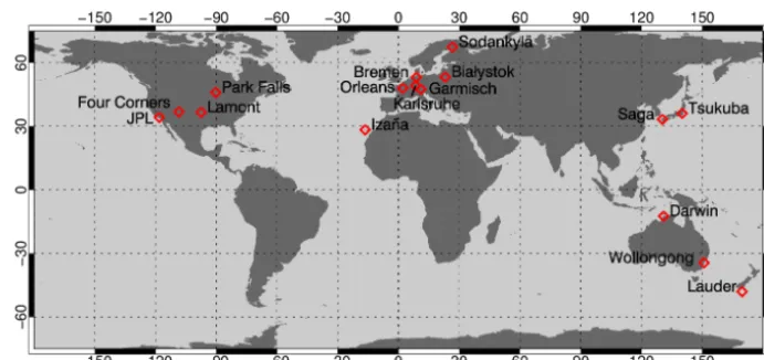
In Fig. 1 a typical example of observed and fitted GOSAT spectra in all three fitting windows is presented. The ob-served and fitted spectra show reasonable agreement. The re-ducedχ2(computed as described by Yoshida et al., 2013) is in all three fitting windows∼1, which means that the dif-ference between observed and fitted spectra agrees with the estimated noise.
5.3 Cloud filtering and post-processing
Table 2. State vector elements of the GOSAT BESD retrieval algorithm.
State vector element Quantities A priori value A priori uncertainty
Albedo 0th polynomial coef. (P0) 3 estimated from computed reflectance 0.1
Albedo 1st polynomial coef. (P1) 3 0.0 0.01
Albedo 2nd polynomial coef. (P2) 3 0.0 0.001
Spectral shift 3 estimated from the position of Fraunhofer lines 0.1 cm−1 Shift of the solar spectrum 3 estimated from the position of Fraunhofer lines 0.1 cm−1
Maximum optical path difference 3 2.5 cm 0.05 cm
Instantaneous field of view 3 15.8 mrad 0.005 mrad
Zero-level offset 1 0.0 (in units 109W cm−2cm sr−1) 1.0
CO2profile 10 based on SECM CO2model see Reuter et al. (2010)
Surface pressure 1 based on ECMWF data 5 hPa
Temperature scaling 1 based on ECMWF data see Reuter et al. (2010)
Water vapour profile scaling 1 based on ECMWF data see Reuter et al. (2010)
Cloud water path 1 1 g m−2 1 g m−2
Cloud top height 1 10 km 2 km
Aerosol profile scaling 1 1.0 0.2
Table 3. Parameters and thresholds as used for the quality filtering. A scene is considered to be of “good” quality if e.g. the albedo difference between the fitted and a priori albedo in band 2 (albedo difference, weak CO2) is larger than the lower threshold of−0.02 and smaller than the upper threshold of 0.02.
Parameter Lower Upper
threshold threshold
Number of iterations – 16
Albedo difference (weak CO2) −0.02 0.02 Albedo second polynomial coef. (weak CO2) – 0.0003
Albedo slope (strong CO2) – −0.003
Albedo second polynomial coef. (strong CO2) −0.0005 –
χ2(O2-A) – 1.2
χ2(weak CO2) – 2.0
χ2(strong CO2) – 2.2
RMSE (weak CO2) – 0.007
Error reduction 0.92 –
XCO2uncertainty – 2.6 ppm
IFOV (O2-A) 15.35 mrad 15.9 mrad
IFOV (weak CO2) 15.5 mrad –
Surface pressure difference −30 hPa 20 hPa
Air-mass factor – 3.5
Viewing zenith angle – 40◦
photons are absorbed by tropospheric water vapour. When a cirrus cloud is located above most of the atmospheric water vapour, a significant amount of radiation can be backscat-tered and measured. A cloud is detected when the measured intensity is larger than a threshold. We use 4 times the mea-surement noise as threshold, which has been empirically de-termined. This filter is sensitive to high ice clouds but not that sensitive to low water clouds. Therefore, we also fil-ter for bright scenes by using the a priori P0 (zeroth-order polynomial coefficient of the albedo) obtained from GOSAT reflectances (see Sect. 5.1). If the a priori P0is larger than a threshold, the measurement is considered to be cloud con-taminated. The threshold for this filter is 0.7 and has also been empirically determined. In addition to these cloud fil-ters, the quality filtering removes still remaining potentially cloud-contaminated scenes.
The high demands on the satellite retrievals require strict quality filtering not only for clouds. In order to minimise bi-ases and to reduce the scatter of the data, GOSAT BESD uses filter thresholds for selected parameters. The used parameters and their filter thresholds have been selected by evaluating GOSAT XCO2 biases and are shown in Table 3. These pa-rameters include e.g. papa-rameters defining the quality of the spectral fit (χ2, RMSE), scattering parameters (CWP, APS) and parameters defining the meteorological state (difference between fitted and a priori surface pressure).
Systematic errors have been additionally reduced by using a global bias correction scheme (similar as done by Schneis-ing et al., 2013; Wunch et al., 2011b; Guerlet et al., 2013). We use TCCON data from all stations listed in Table 4 for the evaluation of the coefficients of the bias correction. As TCCON is used here as reference, the differences to
TC-Table 4. Used TCCON sites, their location, altitude (above sea level) and used observation period.
Station Latitude Longitude Altitude Used observation [◦] [◦] [km] period
Sodankylä 67.37 26.63 0.188 12/02/2009– 26/02/2013 Białystok 53.23 23.03 0.180 01/03/2009–
30/04/2013 Bremen 53.10 8.85 0.270 24/03/2005–
07/05/2013 Karlsruhe 49.10 8.44 0.120 19/04/2010–
28/05/2013 Orleans 47.97 2.11 0.130 29/08/2009–
07/03/2013 Garmisch 47.49 11.06 0.740 16/07/2007–
28/05/2013 Park Falls 45.95 −90.27 0.440 02/06/2004–
07/12/2013 Four Corners 36.80 −108.48 1.643 10/03/2011–
30/05/2013 Lamont 36.60 −97.49 0.320 06/07/2008–
31/12/2013 Tsukuba 36.05 140.12 0.030 25/12/2008–
11/01/2013 JPL 34.20 −118.18 0.390 01/07/2007–
31/03/2013 Saga 33.24 130.29 0.007 28/07/2011–
26/05/2013 Izaña 28.30 −16.50 2.370 18/05/2007–
23/02/2013 Darwin −12.42 130.89 0.030 01/09/2005–
30/05/2013 Wollongong −34.41 150.88 0.030 26/06/2008–
30/05/2013 Lauder −45.04 169.68 0.370 29/06/2004–
01/12/2013
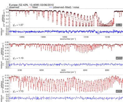
CON can be interpreted as the systematic retrieval errors. Figure 2 shows the dependence of the non-bias-corrected GOSAT BESD–TCCON XCO2differences on the four most relevant retrieval parameters. The four parameters are the viewing zenith angle (VZA), the air-mass factor (AMF),P0 of band 1 (ALB) and the difference to the a prioriP0of band 2 (ALBDIFF). These parameters show a linear or quadratic dependence on these differences.
To reduce the systematic errors in the GOSAT BESD XCO2data set, the following equation has been used: XCOcor2 =XCO2+b0+b1·ALBDIFF+b2·VZA
+b3·VZA2+b4·AMF+b5·AMF2+b6·ALB. (3)
Figure 2. Two-dimensional histograms of non-bias-corrected (left) and standard (bias-corrected, right) GOSAT BESD–TCCON XCO2 differences versus the following four retrieval parameters: (a) viewing zenith angle (VZA), (b) difference of retrieved to a priori albedoP0 of band 2 (ALBDIFF), (c) retrievedP0of band 1 (ALB) and (d) air-mass factor (AMF).
of Fig. 2). Our standard product is the bias corrected GOSAT BESD XCO2data set and the version used here is 01.00.02.
6 Intercomparisons between TCCON, SCIAMACHY and GOSAT XCO2
The quality of the satellite XCO2 data products and their consistency has been assessed using ground-based TCCON XCO2observations. In this section a short overview of TC-CON is given, the assessment method is described and the comparison results are discussed.
6.1 TCCON observations
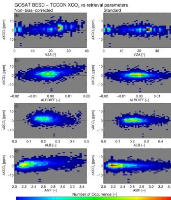
Figure 3. TCCON stations used for validation.
validation that have an overlapping observation period with SCIAMACHY and GOSAT. The used stations are shown in Fig. 3 and listed in Table 4.
6.2 Method
The first part of this study is the validation of the GOSAT BESD (available for January 2010–December 2013) and SCIAMACHY BESD XCO2 (available for August 2003– March 2012) data sets using TCCON XCO2. In order to eval-uate the consistency of the satellite data products, we com-pare the data products with TCCON data for the same time period and perform a direct comparison of the satellite data, i.e. validation results from the overlapping observation years 2010–2011 of SCIAMACHY and GOSAT are presented and compared, and a direct comparison of daily means of the data sets and an additional comparison to daily TCCON data are performed.
The comparison between different CO2 data sets from measurements of different instruments is not trivial because of the different averaging kernels and a priori information as used by the different retrieval algorithms. To ensure that the differences between the measurements are not dominated by differences of the averaging kernels and a priori infor-mation, Rodgers (2000) recommends adjusting the measure-ments by using a common a priori profile and accounting for the averaging kernels. As SCIAMACHY BESD and GOSAT BESD already use the same a priori profiles obtained from the SECM model (Reuter et al., 2012b), only the TCCON measurements need to be adjusted. However, for TCCON, the CO2 averaging kernels are typically very close to unity and the used a priori profiles only marginally differ from the SECM profiles as SECM is based on CarbonTracker CO2 (Peters et al., 2007), which is similar to the TCCON a priori. Reuter et al. (2011) found that adjusting the FTS measure-ments results in only small modifications of about 0.1 ppm. This is small compared to the precision of SCIAMACHY and
GOSAT retrievals. Therefore, the FTS measurements are not adjusted.
All TCCON measurements 2 hours before or after the satellite measurement and all satellite data within a 10◦× 10◦box surrounding the TCCON stations are used. We have also tested other collocation criteria such as a 5◦ and a 350 km radius around the TCCON sites. The results of the intercomparison of the data sets using these collocation cri-teria have been similar to the 10◦×10◦box (see Table S1, S2 and S3 in the Supplement). For the results presented here we have decided to use the 10◦×10◦box collocation criterion as it provided the largest amount of collocated data points.
Four values have been obtained from the comparisons of the data sets at the TCCON sites: (i) the number of collo-cated data points, (ii) the mean difference between the data sets (can be interpreted as a regional bias), (iii) the standard deviation of the difference (is an estimate of the precision when compared with TCCON) and (iv) the linear correlation coefficient between the data sets.
6.3 Results
6.3.1 Entire time series
Figure 4 shows time series of BESD and TCCON XCO2at the Lamont and Darwin TCCON sites. The qualitative com-parison between SCIAMACHY BESD and GOSAT BESD XCO2 indicates good consistency between the data sets as the satellite data are in reasonable to good agreement among themselves and with TCCON. This has been further investi-gated by more quantitative comparisons.
SCIA-Figure 4. SCIAMACHY BESD (black), GOSAT BESD (green) and TCCON (red) XCO2at the Lamont (top) and Darwin (bottom) TCCON sites (±2 h, 10◦×10◦).
Figure 5. Scatter plots of individual satellite vs. TCCON XCO2 measurements at the chosen TCCON sites. (a) GOSAT BESD XCO2 (January 2012–December 2013) vs. TCCON XCO2. (b) SCIAMACHY BESD XCO2(August 2002–March 2012) vs. TCCON XCO2.n is the number of collocations,1is the mean difference between the satellite-based data and TCCON,σ is the standard deviation of the difference andris the correlation coefficient.
MACHY. The mean difference to TCCON is −0.38 ppm for GOSAT and −0.11 ppm for SCIAMACHY. The stan-dard deviation of the difference to TCCON is similar (∼ 2 ppm) for GOSAT and SCIAMACHY. The correlation coef-ficient between GOSAT/TCCON is 0.84 and between SCIA-MACHY/TCCON 0.90.
In more detail, the comparison results between GOSAT BESD XCO2 and TCCON are shown in Table 5 (full time series, standard). The standard deviation of the difference is between 1.36 ppm (Darwin) and 2.65 ppm (Karlsruhe); the station bias to TCCON is in the range −0.92 ppm (JPL) to 2.07 ppm (Tsukuba) and the correlation coefficient between GOSAT BESD and TCCON is between 0.57 (JPL) and 0.89 (Park Falls). The comparison results at the Izaña TCCON site should be interpreted with care as some of the collocated
GOSAT data could be measured over scenes with a large altitude difference to the Izaña site (altitude of 2.37 km). Also shown are the results for the non-bias-corrected GOSAT BESD XCO2. Due to the found systematic retrieval errors, the station biases are between−3.56 ppm (Sodankylä) and 1.37 ppm (Tsukuba), the standard deviation of the difference is between 3.35 ppm (Karlsruhe) and 1.94 ppm (Darwin) and the correlation coefficient is between 0.44 (JPL) and 0.82 (Park Falls, Tsukuba).
Table 5. Results of the comparison between GOSAT BESD and TCCON XCO2for individual (single measurement) satellite data. Shown are the results for non-bias corrected and standard (bias-corrected) GOSAT BESD of the full time series (January 2010–December 2013, see Fig. S1 for the time series of the standard GOSAT BESD) of the data set and for a 2010–2011 sub-set of the standard GOSAT BESD data product.1is the mean difference between GOSAT BESD and TCCON XCO2,σ is the standard deviation of the difference,r is the correlation coefficient between the time series andnthe number of collocations. Stations marked with∗have less than 30 collocations in one of the comparisons of GOSAT BESD or SCIAMACHY BESD XCO2with TCCON XCO2. Therefore, these comparisons should be interpreted with care. The mean offset (mean of the mean differences), the estimated single measurement precision (mean of the standard deviation of the difference), the mean correlation coefficient and the station-to-station bias (standard deviation of the mean differences) are calculated without these stations.
Station Full data set 2010–2011
Non-bias-corrected Standard Standard
1[ppm] σ[ppm] r[–] 1[ppm] σ[ppm] r[–] n[–] 1[ppm] σ[ppm] r[–] n[–]
Sodankylä −3.56 2.58 0.71 −0.16 1.97 0.79 37 −0.17 1.93 0.78 32 Białystok −2.41 3.00 0.78 −0.53 2.15 0.88 185 −0.75 2.26 0.78 97
Bremen −1.39 2.38 0.77 −0.88 2.31 0.76 54 −1.01 2.25 0.65 45
Karlsruhe −1.53 3.35 0.64 −0.65 2.65 0.76 271 −0.58 2.67 0.69 173 Orleans −0.98 2.90 0.54 −0.04 2.21 0.69 140 −0.12 2.24 0.66 121
Garmisch −0.47 3.21 0.66 0.60 2.50 0.78 239 0.52 2.30 0.72 159
Park Falls −0.83 2.61 0.82 0.25 1.96 0.89 402 0.19 1.79 0.79 193 Four Corners −1.83 2.66 0.72 −0.36 2.12 0.78 1145 −0.77 2.14 0.68 375 Lamont −2.05 2.51 0.78 −0.48 1.91 0.86 2199 −0.47 1.88 0.77 959
Tsukuba∗ 1.37 2.63 0.82 2.07 2.41 0.85 83 1.16 1.94 0.64 14
JPL∗ −2.65 3.15 0.44 −0.92 2.06 0.57 656 −1.95 2.02 −0.48 14
Saga∗ −1.87 3.30 0.80 0.03 2.26 0.88 43 −0.02 2.52 0.37 20
Izaña∗ −1.36 2.31 0.63 −0.33 2.09 0.64 68 −0.01 2.13 0.52 43 Darwin −2.42 1.94 0.60 −0.64 1.36 0.73 655 −1.00 1.24 0.59 163 Wollongong −2.89 2.91 0.66 −0.43 1.84 0.76 736 −0.43 1.76 0.65 340
Lauder∗ −0.18 3.07 0.62 0.46 1.72 0.80 139 0.33 1.84 0.33 50
MEAN −1.85 2.78 0.69 −0.30 2.09 0.79 −0.42 2.04 0.71
SD 0.93 0.43 0.48
Table 6. As Table 5 but for SCIAMACHY BESD XCO2full data set (August 2003–March 2012, see Fig. S2 for the time series) and for a 2010–2011 sub-set.
Station Full data set 2010–2011
1[ppm] σ[ppm] r[–] n[–] 1[ppm] σ[ppm] r[–] n[–]
Sodankylä 1.11 1.97 0.89 271 1.10 1.77 0.89 171
Białystok 0.23 2.29 0.77 1689 0.13 2.67 0.62 763
Bremen −0.85 2.37 0.87 1788 −1.07 1.68 0.86 667
Karlsruhe −0.61 2.52 0.70 1869 −0.51 2.55 0.65 1728
Orleans 0.26 2.48 0.78 1334 0.42 2.55 0.45 942
Garmisch 1.20 2.43 0.85 1987 0.98 2.51 0.59 906
Park Falls 0.30 2.07 0.93 5375 0.75 1.92 0.71 1663
Four Corners −1.95 2.35 0.38 637 −1.61 2.10 0.37 523
Lamont −0.19 1.89 0.85 16 520 −0.37 1.91 0.67 7204
Tsukuba∗ 2.36 2.35 0.74 62 2.57 2.20 0.37 23
JPL∗ −0.46 2.29 0.88 1016 −0.05 2.02 0.22 64
Saga* 0.06 2.63 0.55 60 −0.32 2.38 0.16 55
Izaña∗ 1.75 2.12 0.81 11 2.66 2.43 0.92 6
Darwin −0.35 1.72 0.85 11 044 −0.87 1.67 0.64 730
Wollongong 0.25 2.09 0.69 4233 0.13 2.04 0.45 2535
Lauder∗ 1.11 3.03 0.90 59 1.31 3.44 0.74 11
MEAN −0.05 2.20 0.78 −0.08 2.12 0.63
correlation coefficient is typically high and is between 0.38 (Four Corners) and 0.93 (Park Falls). The low correlation co-efficient at Four Corners can be explained by the dependence of the correlation coefficient on the length of the time series. At Four Corners SCIAMACHY and TCCON have colloca-tions only in 1 year compared to 8 years at Park Falls. An additional explanation for the low correlation at Four Cor-ners can be the collocation criterion. There are two large power plants in the vicinity of the Four Corners TCCON sta-tion introducing large variability (Lindenmaier et al., 2014) which can be smeared out in the satellite data by using the 10◦×10◦ collocation criterion. This may also be a reason for the large−1.95 ppm mean difference to TCCON at Four Corners.
In order to summarise the results, we calculate the mean standard deviation of the difference (can be interpreted as an upper limit for the single measurement precision) and the standard deviation of the station biases, which we interpret as the station-to-station bias deviation (short: station-to-station bias). For the sake of completeness, we also calculate the mean of the station biases (mean offset) and the mean cor-relation coefficient. However, the mean offset is less relevant as it can be easily adjusted. In order to determine robust val-ues, we have excluded TCCON stations with less than 30 measurements in one of the comparisons, i.e. Tsukuba, JPL, Saga, Izaña and Lauder are not considered.
The full data set analysis (GOSAT: January 2010– December 2013; SCIAMACHY: August 2002–March 2012) shows for the standard GOSAT BESD data set a mean offset of−0.30 ppm, a single measurement precision of 2.09 ppm, a mean correlation coefficient of 0.79 and a station-to-station bias of 0.43 ppm. Compared to the non-bias-corrected GOSAT BESD data set (mean offset of −1.85 ppm, sin-gle measurement precision of 2.78 ppm, mean correlation coefficient of 0.69 and station-to-station bias of 0.93 ppm) the quality of the standard (bias-corrected) GOSAT BESD data set is enhanced as the implemented bias correction scheme reduces systematic retrieval errors. The results for the standard GOSAT BESD data set are similar to results of other XCO2products from retrieval algorithms applied to GOSAT observations; e.g. Dils et al. (2014) found for the full-physics algorithm of the University of Leicester (Co-gan et al., 2012) a mean offset of−0.76 ppm, a single mea-surement precision of 2.37 ppm, a mean correlation coeffi-cient of 0.79 and a station-to-station bias of 0.53 ppm and for SRON’s RemoTeC algorithm (Butz et al., 2011) a mean offset of −0.57 ppm, a mean single measurement precision of 2.50 ppm, a mean correlation coefficient of 0.81 and a station-to-station bias of 0.75 ppm. Note that both data sets are bias corrected as well. They used GOSAT data between April 2009 and April 2011, a collocation time of±2 h and all measurements within a 500 km radius around a TCCON site.
−0.05 ppm, a single measurement precision of 2.20 ppm, a mean correlation coefficient of 0.78 and a station-to-station bias of 0.89 ppm. The mean offset, the mean single measure-ment precision and the mean correlation coefficient are sim-ilar to the findings of Dils et al. (2014). They found a mean offset of 0.02 ppm, a slightly larger single measurement pre-cision of 2.53 ppm and a mean correlation of 0.81. The station-to-station bias found by Dils et al. (2014) is slightly better with 0.63 ppm. A reason for this difference is the large mean difference from TCCON at Four Corners (−1.95 ppm). Without Four Corners the mean offset (0.14 ppm), the mean correlation coefficient (0.82) and the mean single measure-ment precision (2.18 ppm) remain nearly the same, but the station-to-station bias (0.67 ppm) becomes better and similar to the findings of Dils et al. (2014).
6.3.2 Overlapping time series (2010–2011)
For the comparison of the validation results of GOSAT BESD and SCIAMACHY BESD, we have used the time pe-riod 2010 to 2011 where both data sets overlap. Both data sets have a negative station bias e.g. at Bremen (−1.01 ppm for GOSAT and −1.07 ppm for SCIAMACHY), Darwin (−1.00 ppm for GOSAT and−0.87 ppm for SCIAMACHY) and Four Corners (−0.77 and −1.61 ppm) and a positive station bias e.g. at Garmisch (0.52 and 0.98 ppm). These similarities result in a high correlation coefficient of 0.83 between the station biases of SCIAMACHY BESD and GOSAT BESD (considering all stations with a sufficient number of collocations). The standard deviation of the dif-ference at Karlsruhe is in both data sets similarly high (2.67 and 2.55 ppm) and similarly low at Darwin (1.24 ppm for GOSAT and 1.67 ppm for SCIAMACHY).
Overall, the analysis results for the time period 2010–2011 are similar to the results obtained for the full data set analysis. In both comparisons, the mean offset is negative (−0.42 ppm for GOSAT and−0.08 ppm for SCIAMACHY), the single measurement precision is similar (2.04 ppm for GOSAT and 2.12 ppm for SCIAMACHY) and the mean correlation coef-ficient is high (0.71 for GOSAT and 0.63 for SCIAMACHY). The station-to-station bias is slightly better for GOSAT with 0.48 ppm compared to 0.88 ppm for SCIAMACHY.
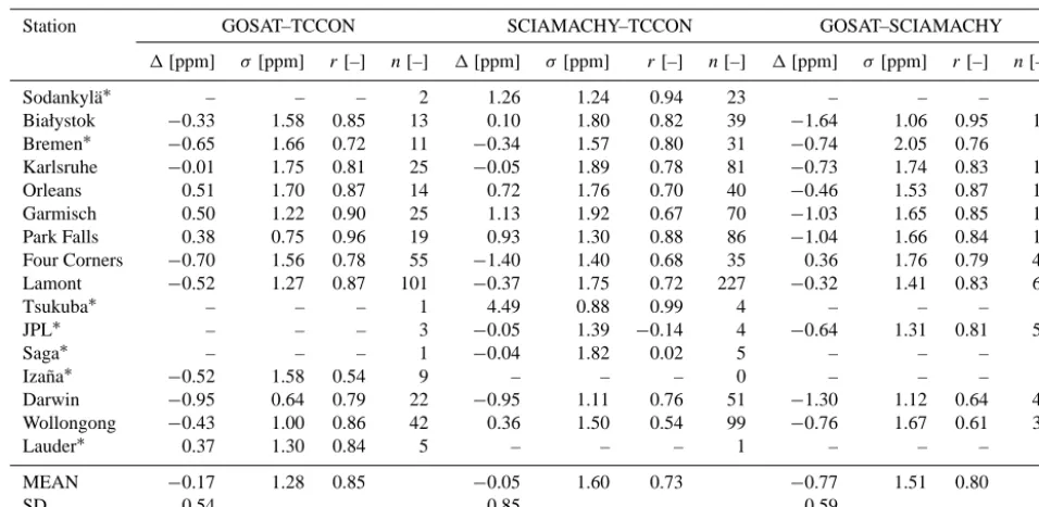
Table 7. Results of the comparison of daily averages of (standard) GOSAT, SCIAMACHY and TCCON XCO2for 2010–2011 (see Fig. S3 for time series). The values are computed as for Table 6. Here, the comparisons at the TCCON sites marked with a∗, with less than 10 days of data for all three comparisons, should be interpreted with care. The mean offset (mean of the mean differences), the estimated single measurement precision (mean of the standard deviation of the difference), the mean correlation coefficient and the station-to-station bias (standard deviation of the mean differences) are calculated without these stations.
Station GOSAT–TCCON SCIAMACHY–TCCON GOSAT–SCIAMACHY
1[ppm] σ[ppm] r[–] n[–] 1[ppm] σ[ppm] r[–] n[–] 1[ppm] σ[ppm] r[–] n[–]
Sodankylä∗ – – – 2 1.26 1.24 0.94 23 – – – 0
Białystok −0.33 1.58 0.85 13 0.10 1.80 0.82 39 −1.64 1.06 0.95 13
Bremen∗ −0.65 1.66 0.72 11 −0.34 1.57 0.80 31 −0.74 2.05 0.76 8
Karlsruhe −0.01 1.75 0.81 25 −0.05 1.89 0.78 81 −0.73 1.74 0.83 14
Orleans 0.51 1.70 0.87 14 0.72 1.76 0.70 40 −0.46 1.53 0.87 18
Garmisch 0.50 1.22 0.90 25 1.13 1.92 0.67 70 −1.03 1.65 0.85 15
Park Falls 0.38 0.75 0.96 19 0.93 1.30 0.88 86 −1.04 1.66 0.84 11
Four Corners −0.70 1.56 0.78 55 −1.40 1.40 0.68 35 0.36 1.76 0.79 43
Lamont −0.52 1.27 0.87 101 −0.37 1.75 0.72 227 −0.32 1.41 0.83 65
Tsukuba∗ – – – 1 4.49 0.88 0.99 4 – – – 0
JPL∗ – – – 3 −0.05 1.39 −0.14 4 −0.64 1.31 0.81 52
Saga∗ – – – 1 −0.04 1.82 0.02 5 – – – 1
Izaña∗ −0.52 1.58 0.54 9 – – – 0 – – – 0
Darwin −0.95 0.64 0.79 22 −0.95 1.11 0.76 51 −1.30 1.12 0.64 40
Wollongong −0.43 1.00 0.86 42 0.36 1.50 0.54 99 −0.76 1.67 0.61 35
Lauder∗ 0.37 1.30 0.84 5 – – – 1 – – – 0
MEAN −0.17 1.28 0.85 −0.05 1.60 0.73 −0.77 1.51 0.80
SD 0.54 0.85 0.59
GOSAT and SCIAMACHY data is small with −0.60 ppm. The standard deviation of the daily difference to TCCON is for GOSAT smaller with 1.37 ppm compared to SCIA-MACHY with 1.79 ppm. The standard deviation of the daily difference between GOSAT and SCIAMACHY is 1.56 ppm, which is similar to the comparison to TCCON. The corre-lation coefficient between GOSAT/TCCON is higher (0.86) compared to SCIAMACHY/TCCON (0.75) and similar to GOSAT/SCIAMACHY (0.82).
A more detailed comparison is shown in Table 7. Only stations with more than 10 days of data are used to com-pute the mean values shown in Table 7. The compari-son with TCCON shows for GOSAT and SCIAMACHY BESD a small negative offset of −0.17 ppm (GOSAT) and −0.05 ppm (SCIAMACHY), a daily precision of 1.28 ppm (GOSAT) and 1.60 ppm (SCIAMACHY), a mean correlation coefficient of 0.85 (GOSAT) and 0.73 (SCIAMACHY) and a station-to-station bias of 0.54 ppm (GOSAT) and 0.85 ppm (SCIAMACHY). The correlation of the daily station biases at the TCCON sites for SCIAMACHY and GOSAT BESD is high (r=0.88). The direct comparison between the GOSAT BESD and SCIAMACHY BESD XCO2data set shows that the satellite data have a −0.77 ppm offset against one an-other. However, this can be simply adjusted by accounting for this offset. The mean scatter of the differences of 1.51 ppm and the mean correlation coefficient of 0.80 are similar to the precision and mean correlation coefficient obtained by the comparison with TCCON. The standard deviation of the
mean differences between GOSAT and SCIAMACHY of 0.59 ppm is smaller/similar than the station-to-station bias of daily GOSAT BESD and SCIAMACHY BESD data.
The differences between the satellite data are likely due to non-perfect collocations (observed air masses are not identi-cal) and potentially due to a non-perfect BESD retrieval al-gorithm. However, the similar scatter of the difference be-tween the data sets compared to the difference to TCCON, the high correlation coefficient of the station biases and the smaller/similar standard deviation of the mean differences of the data sets compared to the station-to-station bias indicate a high degree of consistency between the SCIAMACHY and GOSAT XCO2data sets.
7 Comparisons with CarbonTracker XCO2
Figure 6. As Fig. 5 but for daily averages of GOSAT, SCIA-MACHY and TCCON XCO2 (2010–2011). (a) GOSAT BESD XCO2vs. TCCON XCO2. (b) SCIAMACHY BESD XCO2vs. TC-CON XCO2. (c) GOSAT BESD XCO2vs. SCIAMACHY BESD XCO2.
BESD, SCIAMACHY BESD and CarbonTracker XCO2 have been generated in a grid of 5◦×5◦. All grid boxes with less than 15 measurements have been excluded to achieve ro-bust results. A global mean offset has been added to GOSAT
ter compare the differences to CarbonTracker. From the in-tercomparison of the global maps the mean difference, the standard deviation of the difference and the correlation coef-ficient between the data sets have been computed.
Figure 7 shows the comparison results for April– May 2011. The GOSAT BESD, SCIAMACHY BESD and CarbonTracker maps show a similar strong latitudinal de-pendence of XCO2with high XCO2in the Northern Hemi-sphere and low XCO2 in the Southern Hemisphere. The number of grid boxes filled with sufficient observations is larger for SCIAMACHY than for GOSAT BESD. In com-parison to CarbonTracker, GOSAT BESD as well as SCIA-MACHY BESD has a small mean difference (GOSAT: 0.10 ppm; SCIAMACHY: 0.03 ppm) and a similar stan-dard deviation of the difference (GOSAT: 1.29 ppm; SCIA-MACHY: 1.30 ppm). The correlation coefficient between the BESD data sets and CarbonTracker is similarly high (∼0.9). The direct comparison between GOSAT BESD and SCIA-MACHY BESD shows a mean difference of 0.09 ppm, a smaller standard deviation of the difference of 1.17 ppm and a similar correlation coefficient (r=0.92) as compared to the difference to CarbonTracker. In addition to the global maps, latitudinal averages of the differences are shown (Fig. 7, right panel). Generally the latitudinal differences between the data sets are small. We have also computed the stan-dard deviation of the latitudinal differences (σl). The differ-ences between GOSAT BESD or SCIAMACHY BESD to CarbonTracker show a similarσl(GOSAT: 0.42 ppm; SCIA-MACHY: 0.44 ppm), but the differences between GOSAT and SCIAMACHY BESD are smaller with σl=0.29 ppm. These results show that the north to south dependence of XCO2 is more consistent between the BESD data sets as compared to CarbonTracker.
SCIA-Figure 7. Global maps of XCO2(left), XCO2differences (1XCO2, middle) and latitudinal averages of the differences (right) of GOSAT BESD, SCIAMACHY BESD and CarbonTracker gridded on 5◦×5◦for April–May 2011. The values shown near the bottom of the difference maps are1, the mean difference between the data products,σ, the standard deviation of the difference andr, the correlation coefficient. The black diamonds in the right panels are the XCO2differences in the individual grid boxes. The red triangles represent the latitudinal averages and the error bars the latitudinal standard deviation.σlis the standard deviation over all latitudinal averages.
MACHY: 0.62 ppm). These results again show that the north to south dependence of XCO2is more consistent between the BESD data sets as compared to CarbonTracker.
The remaining differences between GOSAT and SCIA-MACHY BESD are likely due to the non-perfect spatial and temporal collocations and a non-perfect BESD algorithm. However, the smaller/similar differences of the BESD data sets as compared to CarbonTracker are another indication for the high degree of consistency between GOSAT and SCIA-MACHY BESD.
8 Conclusions
As consistent long-term data sets of XCO2are required for carbon cycle and climate-related research, we have investi-gated whether retrievals of XCO2 from different satellites
but evaluated using the same retrieval algorithm are consis-tent. For this purpose, the BESD algorithm originally de-veloped for SCIAMACHY measurements has been modified and used to also evaluate GOSAT measurements.
The quality of the BESD data products was estimated by a validation study using TCCON observations. This com-parison showed that the GOSAT BESD XCO2 data prod-uct has a mean offset of−0.30 ppm, a single measurement precision of 2.09 ppm, a mean correlation coefficient of 0.79 and a station-to-station bias of 0.43 ppm. The SCIAMACHY BESD XCO2data product has a mean offset of−0.05 ppm, a single measurement precision of 2.20 ppm, a mean cor-relation coefficient of 0.78 and a station-to-station bias of 0.89 ppm (0.67 ppm without Four Corners).
Figure 8. As Fig. 7 but for August–September 2011.
data for the same time period and performed a direct com-parison of the satellite data.
The comparison of the validation results for the years 2010–2011, when the observation periods of SCIAMACHY and GOSAT overlap, showed for both data sets a small mean offset (−0.42 ppm for GOSAT,−0.08 ppm for SCIA-MACHY), a similar single measurement precision of 2.04 ppm for GOSAT and 2.12 ppm for SCIAMACHY and a similar mean correlation coefficient for GOSAT (0.71) and SCIAMACHY (0.63). The station-to-station bias for GOSAT is slightly better with 0.48 ppm compared to 0.88 ppm for SCIAMACHY.
The GOSAT BESD and SCIAMACHY BESD XCO2 data show similarities in the comparisons at the TCCON sites. The mean difference from TCCON is at e.g. Bremen (−1.01 ppm for GOSAT and−1.07 ppm for SCIAMACHY) and Darwin (−1.00 ppm for GOSAT and −0.87 ppm for SCIAMACHY) similarly low. Overall, the correlation
coef-ficient between the station biases of both data sets is large (0.83). The single measurement precision has similar small values e.g. at Darwin (1.24 ppm for GOSAT and 1.67 ppm for SCIAMACHY) and a similar high value e.g. at Karlsruhe (2.67 ppm for GOSAT and 2.55 ppm for SCIAMACHY). These similarities, the large correlation coefficient of the sta-tion biases and the similarity of the validasta-tion results give ev-idence that the GOSAT BESD XCO2and the SCIAMACHY BESD XCO2are generally consistent.
dif-ference (0.59 ppm) compared to the difdif-ference to TCCON (0.54 ppm for GOSAT and 0.85 ppm for SCIAMACHY).
We have also compared global monthly maps and lat-itudinal averages of the satellite data sets with Carbon-Tracker XCO2. Results of two time periods, April–May and August–September 2011, were presented. These results showed that the differences between the BESD data sets are smaller/similar as the difference to CarbonTracker.
The remaining differences found between GOSAT and SCIAMACHY are likely not only due to non-perfect col-location (i.e. the observed air masses can be not identical) but likely also to a non-perfect BESD retrieval algorithm. However, the similar scatter of the difference between the data sets compared to the difference to TCCON and Carbon-Tracker and the smaller/similar station-to-station variation of the differences of the data sets compared to the difference to TCCON indicate a high degree of consistency between the SCIAMACHY and GOSAT XCO2 data sets. These results demonstrates that consistent retrievals can be obtained from different satellite instruments using the same retrieval algo-rithm.
Our overarching goal is to generate a satellite-derived XCO2data set appropriate for climate and carbon cycle re-search covering the longest time period. We therefore also plan to extend the existing SCIAMACHY and GOSAT data set discussed here by also using data from other current or future missions, e.g. OCO-2 (Crisp et al., 2004), GOSAT-2 and CarbonSat (Bovensmann et al., 2010; Buchwitz et al., 2013a).
The Supplement related to this article is available online at doi:10.5194/amt-8-2961-2015-supplement.
Acknowledgements. We thank JAXA, NIES and ESA for providing us with the GOSAT L1B and L2 IDS data. We are also grateful to Jonathan de Ferranti for the development of the digital elevation model, which we used for our evaluations. We thank TCCON for providing FTS XCO2 data obtained from the TCCON Data Archive, operated by the California Institute of Technology, from the website at http://tccon.ipac.caltech.edu/. The CarbonTracker CT2013B results has been provided by NOAA ESRL, Boulder, Colorado, USA, from the website at http://carbontracker.noaa.gov. We thank NASA for providing us with the ABSCOv4 tables and ECMWF for the meteorological data. This work has been funded by the EU FP7 (MACC-II), EU Horizon 2020 (MACC-III), ESA (GHG-CCI project and Living Planet Fellowship project CARBOFIRES) and the state and the University of Bremen.
The article processing charges for this open-access publication were covered by the University of Bremen.
Edited by: D. Brunner
References
Aben, I., Hasekamp, O., and Hartmann, W.: Uncertainties in the space-based measurements of CO2columns due to scattering in the Earth’s atmosphere, J. Quant. Spectrosc. Ra., 104, 450–459, doi:10.1016/j.jqsrt.2006.09.013, 2006.
Agustí-Panareda, A., Massart, S., Chevallier, F., Boussetta, S., Bal-samo, G., Beljaars, A., Ciais, P., Deutscher, N. M., Engelen, R., Jones, L., Kivi, R., Paris, J.-D., Peuch, V.-H., Sherlock, V., Vermeulen, A. T., Wennberg, P. O., and Wunch, D.: Forecast-ing global atmospheric CO2, Atmos. Chem. Phys., 14, 11959– 11983, doi:10.5194/acp-14-11959-2014, 2014.
Bovensmann, H., Burrows, J. P., Buchwitz, M., Frerick, J., Noël, S., Rozanov, V. V., Chance, K. V., and Goede, A.: SCIAMACHY – mission objectives and measurement modes, J. Atmos. Sci., 56, 127–150, 1999.
Bovensmann, H., Buchwitz, M., Burrows, J. P., Reuter, M., Krings, T., Gerilowski, K., Schneising, O., Heymann, J., Tret-ner, A., and Erzinger, J.: A remote sensing technique for global monitoring of power plant CO2emissions from space and related applications, Atmos. Meas. Tech., 3, 781–811, doi:10.5194/amt-3-781-2010, 2010.
Buchwitz, M., Rozanov, V. V., and Burrows, J. P.: A correlated-k distribution scheme for overlapping gases suitable for retrieval of atmospheric constituents from moderate resolution radiance measurements in the visible/near-infrared spectral region, J. Geo-phys. Res., 105, 15247–15261, 2000.
Buchwitz, M., Reuter, M., Bovensmann, H., Pillai, D., Heymann, J., Schneising, O., Rozanov, V., Krings, T., Burrows, J. P., Boesch, H., Gerbig, C., Meijer, Y., and Löscher, A.: Carbon Monitoring Satellite (CarbonSat): assessment of atmospheric CO2and CH4 retrieval errors by error parameterization, Atmos. Meas. Tech., 6, 3477–3500, doi:10.5194/amt-6-3477-2013, 2013a.
Buchwitz, M., Reuter, R., Schneising, O., Bösch, H., Guerlet, S., Dils, B., Aben, I., Armante, R., Bergamaschi, P., Blumen-stock, T., Bovensmann, H., Brunner, D., Buchmann, B., Bur-rows, J. P., Butz, A., Chedin, A., Chevallier, F., Crevoisier, C. D., Deutscher, N. M., Frankenberg, C., Hase, F., Hasekamp, O. P., Heymann, J., Kaminski, T., Laeng, A., Lichtenberg, G., De Maziere, M., Noel, S., Notholt, J., Orphal, J., Popp, C., Parker, R., Scholze, M., Sussmann, R. Stiller, G. P., Warneke, T., Zehner, C., Bril, A., Crisp, D., Griffith, D. W. T. Kuze, A., O’Dell, D. W. T., Oshchepkov, S., Sherlock, V., Suto, H., Wennberg, P., Wunch, D., Yokota, T., and Yoshida, Y.: The Greenhouse Gas Climate Change Initiative (GHG-CCI): com-parison and quality assessment of near-surface-sensitive satellite-derived CO2and CH4global data sets, Remote Sens. Environ., online first, doi:10.1016/j.rse.2013.04.024, 2013b.
Burrows, J. P., Hölzle, E., Goede, A. P. H., Visser, H., and Fricke, W.: SCIAMACHY – Scanning Imaging Absorption Spectrometer for Atmospheric Chartography, Acta Astronaut., 35, 445–451, 1995.
of the orbiting carbon observatory to the estimation of CO2 sources and sinks: theoretical study in a variational data assimilation framework, J. Geophys. Res., 112, D09307, doi:10.1029/2006JD007375, 2007.
Cogan, A. J., Bösch, H., Parker, R. J., Feng, L., Palmer, P. I., Blavier, J.-F. L., Deutscher, N. M., Macatangay, R., Norholt, J., Roehl, C., Warneke, T., and Wunch, D.: Atmospheric carbon dioxide retrieved from the Greenhouse gases Observing SATel-lite (GOSAT): comparison with ground-based TCCON obser-ations and GEOS-Chem model calculobser-ations, J. Geophys. Res., 117, D21301, doi:10.1029/2012JD018087, 2012.
Crisp, D., Atlas, R. M., Bréon, F.-M., Brown, L. R., Bur-rows, J. P., Ciais, P., Connor, B. J., Doney, S. C., Fung, I. Y., Jacob, D. J., Miller, C. E., O’Brien, D., Pawson, S., Ran-derson, J. T., Rayner, P., Salawitch, R. S., Sander, S. P., Sen, B., Stephens, G. L., Tans, P. P., Toon, G. C., Wennberg, P. O., Wofsy, S. C., Yung, Y. L., Kuang, Z., Chu-dasama, B., Sprague, G., Weiss, P., Pollock, R., Kenyon, D., and Schroll, S.: The Orbiting Carbon Observatory (OCO) mission, Adv. Space Res., 34, 700–709, 2004.
Crisp, D., Fisher, B. M., O’Dell, C., Frankenberg, C., Basilio, R., Bösch, H., Brown, L. R., Castano, R., Con-nor, B., Deutscher, N. M., Eldering, A., Griffith, D., Gunson, M., Kuze, A., Mandrake, L., McDuffie, J., Messerschmidt, J., Miller, C. E., Morino, I., Natraj, V., Notholt, J., O’Brien, D. M., Oyafuso, F., Polonsky, I., Robinson, J., Salawitch, R., Sher-lock, V., Smyth, M., Suto, H., Taylor, T. E., Thompson, D. R., Wennberg, P. O., Wunch, D., and Yung, Y. L.: The ACOS CO2 retrieval algorithm – Part II: Global XCO2data characterization, Atmos. Meas. Tech., 5, 687–707, doi:10.5194/amt-5-687-2012, 2012.
Dee, D. P., Uppala, S. M., Simmons, A. J., Berrisford, P., Poli, P., Kobayashi, S., Andrae, U., Balmaseda, M. A., Balsamo, G., Bauer, P., Bechtold, P., Beljaars, A. C. M., van de Berg, L., Bidlot, J., Bormann, N., Delsol, C., Dragani, R., Fuentes, M., Geer, A. J., Haimberger, L., H. S. B., Hersbach, H., Hólm, E. V., Isaksen, L., Kållberg, P., Köhler, M., Matricardi, M., Mc-Nally, A. P., Monge-Sanz, B. M., Morcrette, J.-J., Park, B.-K., Peubey, C., de Rosnay, P., Tavolato, C., Thépaut, J.-N., and Vi-tart, F.: The ERA-Interim reanalysis: configuration and perfor-mance of the data assimilation system, Q. J. Roy. Meteor. Soc., 137, 553–597, doi:10.1002/qj.828, 2011.
Dils, B., Buchwitz, M., Reuter, M., Schneising, O., Boesch, H., Parker, R., Guerlet, S., Aben, I., Blumenstock, T., Burrows, J. P., Butz, A., Deutscher, N. M., Frankenberg, C., Hase, F., Hasekamp, O. P., Heymann, J., De Mazière, M., Notholt, J., Suss-mann, R., Warneke, T., Griffith, D., Sherlock, V., and Wunch, D.: The Greenhouse Gas Climate Change Initiative (GHG-CCI): comparative validation of GHG-CCI SCIAMACHY/ENVISAT and TANSO-FTS/GOSAT CO2 and CH4 retrieval algorithm products with measurements from the TCCON, Atmos. Meas. Tech., 7, 1723–1744, doi:10.5194/amt-7-1723-2014, 2014. Guerlet, S., Butz, A., Schepers, D., Basu, S., Hasekamp, O. P.,
Kuze, A., Yokota, T., Blavier, J., Deutscher, N. M., Grif-fith, D. W. T., Hase, F., Kyro, E., Morino, I., Sherlock, V., Suss-mann, R., Galli, A., and Aben, I.: Impact of aerosol and thin cirrus on retrieving and validating XCO2 from GOSAT
short-doi:10.1002/jgrd.50332, 2013.
Heymann, J., Schneising, O., Reuter, M., Buchwitz, M., Rozanov, V. V., Velazco, V. A., Bovensmann, H., and Bur-rows, J. P.: SCIAMACHY WFM-DOAS XCO2: comparison with CarbonTracker XCO2focusing on aerosols and thin clouds, Atmos. Meas. Tech., 5, 1935–1952, doi:10.5194/amt-5-1935-2012, 2012a.
Heymann, J., Bovensmann, H., Buchwitz, M., Burrows, J. P., Deutscher, N. M., Notholt, J., Rettinger, M., Reuter, M., Schneising, O., Sussmann, R., and Warneke, T.: SCIAMACHY WFM-DOAS XCO2: reduction of scattering related errors, At-mos. Meas. Tech., 5, 2375–2390, doi:10.5194/amt-5-2375-2012, 2012b.
Hilker, M.: Influence of the linear-k method on the accuracy and computational efficiency of GOSAT XCO2 retrievals, Atmos. Meas. Tech., in preparation, 2015.
Hollingsworth, A., Engelen, R. J., Benedetti, A., Dethof, A., Flem-ming, J., Kaiser, J. W., Morcrette, J.-J., Simmons, A. J., Tex-tor, C., Boucher, O., Chevallier, F., Rayner, P., Elbern, H., Es-kes, H., Granier, C., Peuch, V.-H., Rouil, L., and Schultz, M. G.: Toward a monitoring and forecasting system for atmospheric composition: the GEMS project, B. Am. Meteorol. Soc., 89, 1147–1164, 2008.
Hollmann, R., Merchant, C. J., Saunders, R., Downy, C., Buchwitz, M., Cazenave, A., Chuvieco, E., Defourny, P., de Leeuw, G., Forsberg, R., Holzer-Popp, T., Paul, F., Sand-ven, S., Sathyendranath, S., van Roozendael, M., and Wag-ner, W.: The ESA climate change initiative: satellite data records for essential climate variables, B. Am. Meteorol. Soc., 94, 1541– 1552, doi:10.1175/BAMS-D-11-00254.1, 2013.
Houweling, S., Breon, F.-M., Aben, I., Rödenbeck, C., Gloor, M., Heimann, M., and Ciais, P.: Inverse modeling of CO2sources and sinks using satellite data: a synthetic inter-comparison of mea-surement techniques and their performance as a function of space and time, Atmos. Chem. Phys., 4, 523–538, doi:10.5194/acp-4-523-2004, 2004.
Houweling, S., Hartmann, W., Aben, I., Schrijver, H., Skidmore, J., Roelofs, G.-J., and Breon, F.-M.: Evidence of systematic errors in SCIAMACHY-observed CO2due to aerosols, Atmos. Chem. Phys., 5, 3003–3013, doi:10.5194/acp-5-3003-2005, 2005. Hungershoefer, K., Breon, F.-M., Peylin, P., Chevallier, F.,
Rayner, P., Klonecki, A., Houweling, S., and Marshall, J.: Eval-uation of various observing systems for the global monitoring of CO2surface fluxes, Atmos. Chem. Phys., 10, 10503–10520, doi:10.5194/acp-10-10503-2010, 2010.
Kuze, A., Suto, H., Nakajima, M., and Hamazaki, T.: Thermal and near infrared sensor for carbon observation Fourier-transform spectrometer on the Greenhouse Gases Observing Satellite for greenhouse gases monitoring, Appl. Optics, 48, 6716–6733, 2009.
Lindenmaier, R., Dubey, M. K., Henderson, B. G., Zachary, T. B., Herman, J. R., Rahn, T., and Lee, S.-H.: Multiscale observations of CO2,13CO2, and pollutants at Four Corners for emission ver-ification and attribution, P. Natl. Acad. Sci. USA, 111, 8386– 8391, doi:10.1073/pnas.1321883111, 2014.
Palm, M., Ramonet, M., Rettinger, M., Schmidt, M., Suss-mann, R., Toon, G. C., Truong, F., Warneke, T., Wennberg, P. O., Wunch, D., and Xueref-Remy, I.: Calibration of TCCON column-averaged CO2: the first aircraft campaign over Euro-pean TCCON sites, Atmos. Chem. Phys., 11, 10765–10777, doi:10.5194/acp-11-10765-2011, 2011.
Miller, C. E., Crisp, D., DeCola, P. L., Olsen, S. C., Rander-son, J. T., Michalak, A. M., Alkhaled, A., Rayner, P., Ja-cob, D. J., Suntharalingam, P., Jones, D. B. A., Denning, A. S., Nicholls, M. E., Doney, S. C., Pawson, S., Boesch, H., Connor, B. J., Fung, I. Y., O’Brien, D., Salawitch, R. J., Sander, S. P., Sen, B., Tans, P., Toon, G. C., Wennberg, P. O., Wofsy, S. C., Yung, Y. L., and Law, R. M.: Precision re-quirements for space-based XCO2 data, J. Geophys. Res., 112,
D10314, doi:10.1029/2006JD007659, 2007.
O’Dell, C. W., Connor, B., Bösch, H., O’Brien, D., Frankenberg, C., Castano, R., Christi, M., Eldering, D., Fisher, B., Gunson, M., McDuffie, J., Miller, C. E., Natraj, V., Oyafuso, F., Polon-sky, I., Smyth, M., Taylor, T., Toon, G. C., Wennberg, P. O., and Wunch, D.: The ACOS CO2 retrieval algorithm – Part 1: De-scription and validation against synthetic observations, Atmos. Meas. Tech., 5, 99–121, doi:10.5194/amt-5-99-2012, 2012. Oshchepkov, S., Bril, A., and Yokota, T.: PPDF-based method to
account for atmospheric light scattering in observations of car-bon dioxide from space, J. Geophys. Res.-Atmos., 113, D23210, doi:10.1029/2008JD010061, 2008.
Peters, W., Jacobson, A. R., Sweeney, C., Andrews, A. E., Con-way, T. J., Masarie, K., Miller, J. B., Bruhwiler, L. M. P., Petron, G., Hirsch, A. I., Worthy, D. E. J., van der Werf, G. R., Randerson, J. T., Wennberg, P. O., Krol, M. C., and Tans, P. P.: An atmospheric perspective on North American carbon dioxide exchange: CarbonTracker, P. Natl. Acad. Sci. USA, 104, 18925– 18930, doi:10.1073/pnas.0708986104, 2007.
Rayner, P. J. and O’Brien, D. M.: The utility of remotely sensed CO2 concentration data in surface inversions, Geo-phys. Res. Lett., 28, 175–178, 2001.
Reuter, M., Buchwitz, M., Schneising, O., Heymann, J., Bovens-mann, H., and Burrows, J. P.: A method for improved SCIA-MACHY CO2retrieval in the presence of optically thin clouds, Atmos. Meas. Tech., 3, 209–232, doi:10.5194/amt-3-209-2010, 2010.
Reuter, M., Bovensmann, H., Buchwitz, M., Burrows, J. P., Connor, B. J., Deutscher, N. M., Griffith, D. W. T., Hey-mann, J., Keppel-Aleks, G., Messerschmidt, J., Notholt, J., Petri, C., Robinson, J., Schneising, O., Sherlock, V., Velazco, V., Warneke, T., Wennberg, P. O., and Wunch, D.: Retrieval of atmospheric CO2 with enhanced accuracy and precision from SCIAMACHY: validation with FTS measurements and com-parison with model results, J. Geophys. Res., 116, D04301, doi:10.1029/2010JD015047, 2011.
Reuter, M., Bovensmann, H., Buchwitz, M., Burrows, J., Deutscher, N., Heymann, J., Rozanov, A., Schneising, O., Suto, H., Toon, G., and Warneke, T.: On the potential of the 2041–2047 nm spectral region for remote sensing of atmospheric CO2 isotopologues, J. Quant. Spectrosc. Ra., 12, 2009–2017, 2012a.
Reuter, M., Buchwitz, M., Schneising, O., Hase, F., Heymann, J., Guerlet, S., Cogan, A. J., Bovensmann, H., and Burrows, J. P.: A simple empirical model estimating atmospheric CO2
background concentrations, Atmos. Meas. Tech., 5, 1349–1357, doi:10.5194/amt-5-1349-2012, 2012b.
Reuter, M., Bösch, H., Bovensmann, H., Bril, A., Buch-witz, M., Butz, A., Burrows, J. P., O’Dell, C. W., Guer-let, S., Hasekamp, O., Heymann, J., Kikuchi, N., Oshchep-kov, S., Parker, R., Pfeifer, S., Schneising, O., Yokota, T., and Yoshida, Y.: A joint effort to deliver satellite retrieved atmo-spheric CO2concentrations for surface flux inversions: the en-semble median algorithm EMMA, Atmos. Chem. Phys., 13, 1771–1780, doi:10.5194/acp-13-1771-2013, 2013.
Reuter, M., Bovensmann, H., Buchwitz, M., Burrows, J. P., Hey-mann, J., Hilker, M., and Schneising, O.: Algorithm Theoreti-cal Basis Document Version 3 – The Bremen Optimal Estima-tion DOAS (BESD) algorithm for the retrieval of XCO2– ESA Climate Change Initiative (CCI) for the Essential Climate Vari-able (ECV), Tech. rep., University of Bremen, availVari-able at: http: //www.esa-ghg-cci.org (last access: 18 December 2014), 2014a. Reuter, M., Buchwitz, M., Hilboll, A., Richter, A., Schneising, O., Hilker, M., Heymann, J., Bovensmann, H., and Burrows, J. P.: Decreasing emissions of NOxrelative to CO2in East Asia in-ferred from satellite observations, Nat. Geosci., 7, 792–795, doi:10.1038/ngeo2257, 2014b.
Reuter, M., Buchwitz, M., Hilker, M., Heymann, J., Schneising, O., Pillai, D., Bovensmann, H., Burrows, J. P., Bösch, H., Parker, R., Butz, A., Hasekamp, O., O’Dell, C. W., Yoshida, Y., Gerbig, C., Nehrkorn, T., Deutscher, N. M., Warneke, T., Notholt, J., Hase, F., Kivi, R., Sussmann, R., Machida, T., Matsueda, H., and Sawa, Y.: Satellite-inferred European carbon sink larger than expected, Atmos. Chem. Phys., 14, 13739–13753, doi:10.5194/acp-14-13739-2014, 2014c.
Rodgers, C. D.: Inverse Methods for Atmospheric Sounding: The-ory and Practice, World Scientific Publishing, Singapore, 2000. Rothman, L. S., Gordon, I. E., Barbe, A., Benner, D. C.,
Bernath, P. E., Birk, M., Boudon, V., Brown, L. R., Campar-gue, A., Champion, J. P., Chance, K., Coudert, L. H., Dana, V., Devi, V. M., Fally, S., Flaud, J. M., Gamache, R. R., Gold-man, A., Jacquemart, D., Kleiner, I., Lacome, N., Lafferty, W. J., Mandin, J. Y., Massie, S. T., Mikhailenko, S. N., Miller, C. E., Moazzen-Ahmadi, N., Naumenko, O. V., Nikitin, A. V., Or-phal, J., Perevalov, V. I., Perrin, A., Predoi-Cross, A., Rins-land, C. P., Rotger, M., Simeckova, M., Smith, M. A. H., Sung, K., Tashkun, S. A., Tennyson, J., Toth, R. A., Van-daele, A. C., and Vander Auwera, J.: The HITRAN 2008 molec-ular spectroscopic database, J. Quant. Spectrosc. Ra., 110, 533– 572, doi:10.1016/j.jqsrt.2009.02.013, 2009.
Rozanov, V. V., Rozanov, A., Kokhanovsky, A. A., and Bur-rows, J. P.: Radiative transfer through terrestrial atmosphere and ocean: software package SCIATRAN, J. Quant. Spectrosc. Ra., 133, 13–71, doi:10.1016/j.jqsrt.2013.07.004, 2014.
Schneising, O., Bergamaschi, P., Bovensmann, H., Buchwitz, M., Burrows, J. P., Deutscher, N. M., Griffith, D. W. T., Heymann, J., Macatangay, R., Messerschmidt, J., Notholt, J., Rettinger, M., Reuter, M., Sussmann, R., Velazco, V. A., Warneke, T., Wennberg, P. O., and Wunch, D.: Atmospheric greenhouse gases retrieved from SCIAMACHY: comparison to ground-based FTS measurements and model results, Atmos. Chem. Phys., 12, 1527–1540, doi:10.5194/acp-12-1527-2012, 2012.