www.atmos-meas-tech.net/8/1757/2015/ doi:10.5194/amt-8-1757-2015
© Author(s) 2015. CC Attribution 3.0 License.
Bayesian cloud detection for MERIS, AATSR, and
their combination
A. Hollstein1, J. Fischer2, C. Carbajal Henken2, and R. Preusker2
1GeoForschungsZentrum Potsdam (GFZ), Telegrafenberg A17, 14473 Potsdam Germany 2Institute for Space Sciences, Department of Earth Sciences, Freie Universität Berlin, Carl-Heinrich-Becker-Weg 6–10, 12165 Berlin, Germany
Correspondence to: A. Hollstein ([email protected])
Received: 30 September 2014 – Published in Atmos. Meas. Tech. Discuss.: 6 November 2014 Revised: 27 February 2015 – Accepted: 2 March 2015 – Published: 15 April 2015
Abstract. A broad range of different of Bayesian cloud detection schemes is applied to measurements from the Medium Resolution Imaging Spectrometer (MERIS), the Advanced Along-Track Scanning Radiometer (AATSR), and their combination. The cloud detection schemes were de-signed to be numerically efficient and suited for the pro-cessing of large numbers of data. Results from the classical and naive approach to Bayesian cloud masking are discussed for MERIS and AATSR as well as for their combination. A sensitivity study on the resolution of multidimensional his-tograms, which were post-processed by Gaussian smooth-ing, shows how theoretically insufficient numbers of truth data can be used to set up accurate classical Bayesian cloud masks. Sets of exploited features from single and derived channels are numerically optimized and results for naive and classical Bayesian cloud masks are presented. The applica-tion of the Bayesian approach is discussed in terms of repro-ducing existing algorithms, enhancing existing algorithms, increasing the robustness of existing algorithms, and on set-ting up new classification schemes based on manually classi-fied scenes.
1 Introduction
Cloud masking of Earth observation measurements is an im-portant and often crucial part of various remote sensing re-trievals. This includes, but is not limited to, the retrieval of cloud and aerosol microphysical parameters, the estimation of cloud cover, ocean color retrievals, and in general, algo-rithms which include atmospheric correction schemes. Cloud
masking algorithms differ widely in their complexity, com-putational requirements, and assumptions about what a cloud is and which physical process is exploited for their detection. Implementation of particular algorithms are often application specific, which makes the cloud masks as well application specific and generally complicates the inter-comparison of results from different cloud masks.
This paper emphasizes the application of Bayesian meth-ods for the cloud masking of the complete 9.5 year time series of the Medium Resolution Imaging Spectrometer (MERIS) (Rast et al., 1999) and the Advanced Along-Track Scanning Radiometer (AATSR) (Llewellyn-Jones et al., 2001) on-board the Environmental Satellite (ENVISAT) and is part of the European Space Agency (ESA) Cloud CCI (Climate Change Initiative) project (Hollmann et al., 2013). Thus, the requirements for the cloud masking scheme, which is described in Sects. 2 to 5, are robustness, accuracy, and computational efficiency. Several possible applications of the Bayesian method are discussed in Sect. 7. Results for MERIS and AATSR are discussed separately but with a focus on their combination within the Synergy product, in which daytime AATSR measurements are mapped on the MERIS swath and their mutual overlap is used. The Synergy data set in combination with one of the presented cloud detection schemes will be used for the retrieval of cloud microphysi-cal parameters using the FAME-C algorithm which was de-scribed by Carbajal Henken et al. (2014). The development within Cloud CCI is ongoing and finalization of the actual algorithm is planed for the near future.
re-gions and over snow- and ice-covered areas, and the distinc-tion between clouds and optically thick aerosol plumes such as dust storms. These points are discussed in more detail in Sect. 7.
Common approaches to cloud masking are hierarchies of thresholds (e.g., Rossow and Garder, 1993; Schlundt et al., 2011), complex statistical models (e.g., Murtagh et al., 2003; Gómez-Chova et al., 2008), or other Bayesian approaches (e.g., English et al., 1999; Uddstrom et al., 1999; Merchant et al., 2005; Mackie et al., 2010a; Heidinger et al., 2012). A classification scheme for Bayesian cloud masks which helps to clearly distinguish the various approaches to Bayesian cloud masking is introduced in Sect. 3 and, in addition, a short overview of the relevant literature using such schemes is given.
The results presented here are computational highly ef-ficient and are very well suited for the processing of large numbers of data, which makes these results very well suited for future application to the Ocean Land Colour Instrument (OLCI) (Nieke, 2008) and the Sea and Land Surface Temper-ature Radiometer (SLSTR) (Coppo et al., 2010) on-board the Sentinel-3 satellite (Miguel et al., 2007) and its operational follow-ups.
2 Bayesian inference for cloud masking
Bayes’ theorem can be used to reverse joint probabilities. It is appealing to apply it to cloud masking since its theory is widely adopted, its implementation on a computer system is straightforward, and its results are probabilities which can be directly interpreted. The theorem allows the computation of the probabilityP (C,F)that a particular measurement with feature F is affected by a cloud when the occurrence prob-abilities P (F, C) andP (F,C)¯ of the feature under cloudy and non-cloudy conditions are known. Here,P (a, b)denotes the occurrence probability of a under the condition of the occurrence ofb.
WithC being the case that a measurement is affected by clouds andFbeing a set of features associated with that mea-surement,P (C,F)can be expressed as
P (C,F)=P (C)P (F, C) P (F)
= P (C)P (F, C)
P (C)P (F, C)+P (C)P (¯ F,C)¯ , (1) whereP (C)is the background probability of cloudiness and
¯
C is the negation ofC, which states that a measurement is not affected by clouds. The occurrence probability of the feature P (F)can be expressed in terms of the joint proba-bilitiesP (F, C)andP (F,C)¯ , because cloudiness and non-cloudiness are the only two considered classes for each mea-surement.
Evaluating Bayes’ theorem involves only a few arithmetic operations so that a specific implementation can be very fast
and efficient, which is of importance when large numbers of data are to be processed. Additional computations involve the featureF and the a priori joint probabilitiesP (F, C)and P (F,C)¯ , which are discussed in the following sections.
With an appropriate set of thresholds, one can convert the probability P (C,F) into a cloud mask. For instance, any probability strictly higher than 50 % could be interpreted as cloud, but other thresholds or more classes can be used. This is discussed in more detail in Sect. 7.1, but this choice clearly depends on the target application and is independent of the Bayesian approach. Other applications, such as the construc-tion of a cost funcconstruc-tion as described by English et al. (1999), are also viable alternatives.
Estimating the value of the background probabilityP (C) is not discussed in detail in this paper and for all follow-ing applications a value of 0.5 is used. This choice basi-cally states that for each measurement an equal probability of it being cloudy or not cloudy is assumed. This assumption is of course valid neither on a global nor local scale, and a rich body of knowledge about the spatial and temporal distri-bution of cloud occurrence probabilities exists. Such knowl-edge, typical in the form of external climatologies, could be used to estimateP (C)but would eventually shift derived cli-matologies towards the external one, which would then ef-fectively lead to circular arguments. This point might be of lower importance for some applications, i.e., operational pro-cessing by weather services, but within Cloud CCI climato-logical data sets will be derived from the full MERIS and AATSR time series and circular arguments are best to be avoided. Since a decision for the actual value ofP (C)has to be made, its impact on derived data sets should be inves-tigated and communicated to potential users. In general, the background probability can be a function of external or auxil-iary data like position or time of year. In the general case, the estimation of the joint probabilitiesP (F, C) andP (F,C)¯ should be consistent withP (C).
For the special case ofP (C)=0.5, Eq. (1) simplifies to
P (C,F)= P (F, C)
P (F, C)+P (F,C)¯ . (2)
Setting up a particular Bayesian cloud mask algorithm in-volves several decisions, such as specifying the measurement featureFand choosing a technique to estimateP (F, C)and P (F,C)¯ , which allows us to group the various possible ap-proaches to Bayesian cloud masking into distinct subgroups. This natural grouping allows to clearly separate the presented approach from other algorithms and is discussed in Sect. 3. In addition, a short overview about the relevant literature is given.
3 Classification of Bayesian cloud masks
between the various algorithms are often buried in the tech-nical details of the particular paper. A nomenclature which aims to clearly separate different approaches to Bayesian cloud masking is discussed in the following.
Let the featureF from Eq. (1) be a set ofnF real num-bersF=(F1, . . ., FnF)∈R
nF, where theF
iare typically de-termined from measurements M∈RnM, auxiliary data A∈ RnA, and external data E∈RnE. The components F
i are
computed from prescribed feature functionsfi, which gen-erally depend on all of the above introduced classes of data: Fi=fi(M,A,E). In the case of the MERIS and AATSR Synergy, the set of measurementsM includes radiances and brightness temperatures for a single collocated pixel. Auxil-iaryAdata are available with negligible computational cost, such as time stamps, geolocation, and data flags. External data may be a function of the available measurementsMand auxiliary dataAand their procurement are by definition asso-ciated with non-negligible computational cost. This category essentially introduces significant external knowledge about the measurement and common examples are online radiative transfer (RT) simulations, nontrivial interpolation in numeri-cal weather prediction (NWP) data, or the use of climatolo-gies.
Let us call the feature setF independent when it is only a function of the measurementsM and auxiliary dataAand dependent when external dataE are additionally exploited. Both classes can be further subdivided with respect to weak and strong dependence to describe F even more precisely. A weakly dependent feature set could, for example, depend on interpolation in NWP data, which is of negligible compu-tational cost, while a strongly dependent feature set could depend on online RT with non-negligible numerical cost. Strongly independent feature sets would then depend only on measurementsM, while weakly independent feature sets could in addition depend on auxiliary dataA.
This paper focuses on Bayesian cloud masks based on strongly independent features. Only MERIS and AATSR measurements and trivial functions operating on them are used to construct the feature set. This class of features al-lows to implement a numerically highly efficient algorithm with simple opportunities to parallelization and vectoriza-tion. With no dependency on external data, the algorithm can be used in non-operational environments where the acquisi-tion of NWP data can require significant effort. In general, there is no obvious reason why the techniques which are dis-cussed in the following sections are limited to the indepen-dent case.
The second major branch in Bayesian cloud masking schemes involves the computation of the joint probabilities P (F, C) andP (F,C)¯ . The classical approach aims at the direct computation of these two joint probabilities, while the naive approach treats the componentsFiof the feature setF as statistically independent and decouples the joint
probabil-ities onF into a product of joint probabilities of theFi: P (F, C)=Y
i
P (Fi, C). (3)
One can either construct the feature set very carefully, such that this strong assumption holds (e.g., follow Merchant et al. (2005) and their discussion on cloud texture and cloud top temperature), or simply accept its violation and the possible effects on the cloud masking scheme. Formally proving the statement of Eq. (3) seems to be only possible for a rather limited class of features.
Computing the joint probabilities in the classical approach can be greatly simplified by assuming an analytic form and estimating its parameters. Depending on the assumed form, for instance multivariate Gaussian (e.g., see Uddstrom et al., 1999; Merchant et al., 2005), the resulting cloud mask could be called classical Gaussian. As for the naive approach, it will be difficult to formally prove the validity of such as-sumptions.
The classical and naive approaches can be mixed when one or more subsets of theFiare treated as statistically inde-pendent, such that the decoupling ofP (F, C)andP (F,C)¯ becomes partial. For this class of Bayesian cloud masks we propose using the terms “mostly naive” when the majority of features are decoupled and “mostly classical” when the majority of features are not decoupled.
This paper is mainly concerned with the discussion of the classical and naive approach with an emphasis on the classi-cal one. In conclusion, this paper is mostly concerned with the application of classical Bayesian cloud masks based on strongly independent features. As it will be shown later in the paper, the classical approach gives better results for the cloud masking in our scenario and the strongly independent feature set was chosen to allow the implementation of a very fast algorithm.
and were separated when computing the joint probabilities. P (C)was estimated from NWP data and the algorithm was discussed with an emphasis on operational NWP centers such that these feature are likely only weakly dependent. Mackie et al. (2010a, b) discussed a mostly classical Bayesian algo-rithm with strongly dependent features for the 3.9, 11, and 12 µm channel of the SEVIRI instrument. External knowl-edge is introduced by NWP data, and a fast radiative trans-fer model and textural features were separated from spectral features assuming independence. Heidinger et al. (2012) dis-cussed a naive Bayesian cloud mask with strongly dependent features for the AVHRR instrument. A surface type classifi-cation using external MODIS data was used to maximize the detection rate. CALIPSO lidar measurements were used as truth data to compute histograms from which the occurrence probabilities for each feature were estimated.
4 Construction of feature sets
Channels of the MERIS and AATSR instruments cover the spectral range from 412 nm to 12 µm and are referenced in this paper by their central wavelength, while for MERIS the unit of nm and for AATSR the unit µm is used. Figures 1 and 2 show examples of possible features for two particu-larly interesting scenes over Greenland and in the vicinity of the Korean peninsula. Each figure shows an RGB im-age, various single channels, and a selection of trivial func-tions which combine two channels. Both figures include a panel with results of the non-Bayesian Synergy cloud mask, which is briefly discussed in Sect. 6. Figure 1 shows a scene over Greenland with its center located at 59◦3101200W and 79◦00000N with high and low clouds over a large ice- or snow-covered region. Figure 2 shows a scene in the vicinity of the Korean peninsula with its center located at 125◦5201200E and 37◦4503600N. This scene shows a pronounced dust storm mixed with a deck of clouds.
Strongly independent features are constructed using a sin-gle channel or any combination of channels in a trivial func-tion. Such combinations have been called derived channels in the literature (e.g., Uddstrom et al., 1999). Considered here are all basic arithmetic operations (+,−,×, /) and, in addi-tion, the index function dx(a, b)=(a−b)/(a+b), which can be used to create indices such as the normalized difference vegetation index (see Kriegler et al., 1969), the normalized difference snow index (see Hall et al., 2002), or other gen-eral channel indices. Even when well-known and gengen-erally accepted combinations of channels and indices are used, it is unclear whether a specific combination is the best possible candidate for the particular data set and one has to rely on the experience of the involved experts.
In contrast to approaches based on expert knowledge, an objective measure for any given set of feature functions is ex-ploited to numerically search for the best possible set of fea-ture functions. Maximizing the Hanssen–Kuipers skill score
Figure 1. Several views of a scene over Greenland from 17 July 2007 with the image centered at 59◦3101200W and 79◦00000N. Sin-gle panels include a pseudo RGB view, results of the non-Bayesian Synergy cloud mask (with white indicating clouds; see Sect. 6), as well as single channels and simple functions operating on two chan-nels. The function dxdenotes the index function and is defined as dx(a, b)=(a−b)/(a+b). Units are not shown and the color scales are stretched to maximize the visible contrast.
Figure 2. Similar to Fig. 1 but for a scene near the Korean penin-sula. The center of the images is located at 125◦5201200E and 37◦4503600N.
Validation of cloud masks for MERIS and AATSR on-board ENVISAT is a difficult task since no generally ac-cepted and available set of truth data exists. A generally used approach is to generate truth data by means of manual classi-fication of images by human experts or the use of data from ground-based stations. Converting a ground truth to a pixel-by-pixel truth can be complicated, and possibly insufficient spatial coverage can limit the applicability of that approach. Consequently, most approaches for generating truth data for MERIS and AATSR are based on the manual classification of sample data by human experts (e.g., Gómez-Chova et al., 2006, 2008; Schlundt et al., 2011). Such data sets can be called artificial truth because, although they are used as if they were truth, it is arguable whether such data sets are in fact truth.
To demonstrate the feasibility of the Bayesian approach, results from the Synergy cloud mask (see Gómez-Chova et al. (2008) and Sect. 6 for a brief description) were cho-sen as a source of artificial truth data; it is therefore assessed whether Bayesian cloud masks can reproduce this Synergy cloud mask. The major advantage of this approach is that large numbers of artificial truth data can be created without significant effort. Clearly, all shortcomings of this seeding algorithm will be present in this data set and will limit the success of the application of the Bayesian technique.
Optimizing the choice for a particular set of feature func-tions is not straightforward, since this problem is noncontinu-ous with a varying number of free parameters. First, the num-ber of feature functions has to be set. Then, for each feature, a feature function from the pool of considered functions has to be selected. The identity function, all four basic arithmetic operations, and the index function are considered as feature functions. As a last step, the input channels for each feature function must be set. Depending on the chosen functions and channels, a maximum of 2×nF channels can be included in the computation of a feature set withnF elements.
Then, for a particular feature set, the prerequisites for com-puting the joint probabilities must be carried out, which is de-scribed in detail in Sect. 5. Once this step is completed, the Hanssen–Kuipers skill score for the selected set of validation data can be computed.
The only numeric optimization procedure that we are aware of, which is generally applicable to this situation, is a random search in the huge search space spanned by this outlined procedure. This is quite a different approach to that of a human expert, who would likely start an educated search but might not attempt to cover the whole search space. The number of possible combinations depends on the number of chosen features and the number of available channels (22 in the case of the MERIS and AATSR Synergy) and can be es-timated using the binomial coefficient. In the simplest case, where merely the identity function is used, no channel is used more than once, and four features are to be selected, the search space spans224=7315 elements. When only
func-tions of two channels are to be selected and re-selected and channels can be used multiple times, then the search space consists of5×(2242−22)=
2310
4
≈1.2×10¹²entries. The enormous size of the search space makes it difficult to com-pletely cover it by a search, but the random search can be al-lowed to run appropriately long such that a result of sufficient quality is obtained. One can expect that a large number of dif-ferent sets of feature functions will essentially exhibit very similar classification skills. The considered feature functions are not symmetric under a change of the parameter order, but the overall classification result might be approximately sym-metric. This alone would decrease the search space by a fac-tor of approximately 16. In addition, the classification results might be only weakly dependent with respect to the feature function itself; i.e., the index function dx(a, b)might be as effective as a ratioa/b, which would decrease the effective size of the search space.
The proposed random search might not be able to cover the complete search space, but with a sufficiently long run-time one will be able to find solutions with a sufficiently high skill score. In addition, unusual combinations of chan-nels might be found which would not be considered in an educated search by a human expert. The features shown in Figs. 1 and 2 are frequently found in searches when results from the non-Bayesian Synergy cloud mask are used as arti-ficial truth.
The physical meaning of a certain feature set and why it might be better or worse than a different one is not dis-cussed here and is also not within the scope of this paper. This knowledge is very useful for educated searches but is not necessarily needed in this setup. However, for the experi-enced expert it might be only slightly surprising which chan-nels are found to be successful by the optimization scheme. There is also no apparent reason why human experts should not compete with the optimization scheme in order to find an optimum set of features. This is especially important for applications where only a small fraction of the search space can be tested using the optimization approach.
Implementing such a search strategy is straightforward. A generator of random feature functions must be implemented and each of these instances can be tested for its skill score with respect to the artificial truth. This procedure is easily parallelizable, and one could store only the results with a higher skill score rather than some predefined value. At any given time during an ongoing search, one can sort these re-sults and evaluate the top rere-sults.
5 Estimation of background joint probabilities
probability density histograms are produced, from which the probabilities are estimated. In the naive Bayesian approach, as many one-dimensional histograms as there are features are needed, while in the classical Bayesian approach a single nF-dimensional histogram is used. When these histograms are stored in a computer system, the handling of any reason-able number of one-dimensional histograms poses no spe-cific problem, while an array of dimensionnF grows rapidly in memory with increasing number of binsnB. For the sake of simplicity, the same number of bins is assumed for each particular dimension. With four bits per float and twenty bins per feature, one would need 0.6 Gb to store a single his-togram for four features but already about 4883 Gb for seven features. This limits the practical number of features for the classical Bayesian approach to about four to six at the time of writing this paper.
However, the main argument of Uddstrom et al. (1999) and Heidinger et al. (2012) against the use of the classical ap-proach is that one has generally not enough truth data avail-able to robustly derive the histograms in a completely fre-quentist way. This can be a valid point for real truth data, which are limited in principle, but not so much for artifi-cial truth data. Here, the number of available data is merely a function of the available human labor for manual classi-fication or computational resources when an existing cloud masking scheme is used to produce artificial truth data.
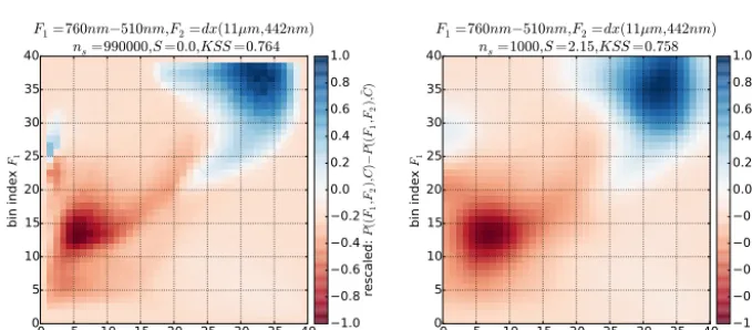
Both left panels of Fig. 3 and 4 show results of two-dimensional histograms for MERIS and AATSR Synergy data. For both cases, almost 1 million spectra were used to compute both histograms. Shown is the difference between the histograms forCandC¯. Both choices of features recreate the Synergy cloud mask reasonably well with a skill score of about 0.76. The cloud masking setup is discussed in detail in Sect. 7. The main point here is that with enough data points these histograms can be computed. The two-dimensional case was chosen since this is simple to visualize.
Both right panels of Figs. 3 and 4 show remarkably similar histograms with just barely smaller skill score values of about 0.75, but only 1000 randomly selected measurements from the original data set were used to produce these histograms. A simple Gaussian smoothing filter was applied to both his-tograms and each Gaussian smoothing factor was chosen such that the skill score as a function of the Gaussian smooth-ing was maximized. This is the first main result of this paper. This numerical experiment shows that, at least for some sets of feature functions, thenF-dimensional histograms can be approximated by using very few data points and an appropri-ate Gaussian smoothing factor. The best smoothing factor for both cases is slightly different and is obtained from optimiza-tion. More detailed results are shown in Sect. 7.1. In addition to the previously discussed parameters, e.g., the construction of features, classical Bayesian cloud masks are defined by the number of bins used in the histograms and the chosen Gaus-sian smoothing parameter, which is discussed in Sect. 7.1.
It should be noted that this is an extreme case and we do not propose to use so few data points to construct cloud masks for real-world applications. These two examples merely show how well this approach operates and that a sur-prisingly small number of data might be sufficient to explore the application of classical Bayesian cloud masks.
The Gaussian smoothing approach works reasonably well and is so far only justified by its actual success for a partic-ular problem, where in fact sufficient numbers of artificial truth data are available. Its general application to situations with limited numbers of such data is therefore not very well justified. However, numerical experiments with the available data have shown that this approach yields remarkably good results. Other functional kernels have not been tested, but the Gaussian approach seems sufficient since the convoluted histograms yield nearly the same skill score as the original histograms. Success of this approach is likely based on the fact that the smoothing procedure distributes data to neigh-bor bins but does not strongly change the defining spectral features of the measurements. That is, it implicitly creates data which could represent different viewing geometries or situations with slightly varying optical parameters. Hence, this approach is not justified by first principles but rather with working examples which strengthen our expectations that this approach will work reasonably well for any other set of features.
6 Synergy cloud mask
The Synergy cloud mask is discussed in detail by Gómez-Chova et al. (2008) and is implemented as an external pro-cessor for the BEAM toolbox (Fomferra and Brockmann, 2005). It is based on radiative transfer simulations covering all spectral bands of MERIS and AATSR and statistical anal-ysis of classified data by human experts. Within the frame of the ESA Cloud CCI project phase 1, the years 2007–2009 of the MERIS and AATSR time series were processed. The derived cloud cover (or cloud number) was assessed in sev-eral validation exercises, e.g., compared to cloud numbers from the GEWEX CA database (Stubenrauch et al., 2012), which consists of a number of data sets with gridded and monthly mean cloud number derived from a variety of satel-lite instruments. Results of global mean cloud number are in line with GEWEX cloud numbers (Hollmann and Lecomte, 2013). The cloud mask product from the years 2007 to 2009 can be used as a large source of artificial truth data for the synergy data set.
7 Application to MERIS, AATSR, and their synergistic product
Re-0 5 10 15 20 25 30 35 40 bin index F2
0 5 10 15 20 25 30 35 40 bin in de x F1
F1=753nm−865nm,F2=dx(442nm,12µm) ns=990000,S=0.0,KSS=0.768
1.0 0.8 0.6 0.4 0.2 0.0 0.2 0.4 0.6 0.8 1.0 re sc ale d: P (( F1 ,F2 ) ,C ) − P (( F1 ,F2 ) ,
¯C)
0 5 10 15 20 25 30 35 40 bin index for F2
0 5 10 15 20 25 30 35 40 bin in de x F1
F1=753nm−865nm,F2=dx(442nm,12µm) ns=1000,S=1.84,KSS=0.759
1.0 0.8 0.6 0.4 0.2 0.0 0.2 0.4 0.6 0.8 1.0 re sc ale d: P (( F1 ,F2 ) ,C ) − P (( F1 ,F2 ) ,
¯C)
Figure 3. Difference of the two-dimensional histograms forP (F, C)andP (F,C). The left panel show a direct results using 990 000 globally¯ distributed measurements, while for the right panel only 1000 measurements were used. The histograms on the right side were post-processed using Gaussian smoothing with a width parameter of 1.84.
0 5 10 15 20 25 30 35 40 bin index F2
0 5 10 15 20 25 30 35 40 bin in de x F1
F1=760nm−510nm,F2=dx(11µm,442nm) ns=990000,S=0.0,KSS=0.764
1.0 0.8 0.6 0.4 0.2 0.0 0.2 0.4 0.6 0.8 1.0 re sc ale d: P (( F1 ,F2 ) ,C ) − P (( F1 ,F2 ) ,
¯C)
0 5 10 15 20 25 30 35 40 bin index for F2
0 5 10 15 20 25 30 35 40 bin in de x F1
F1=760nm−510nm,F2=dx(11µm,442nm) ns=1000,S=2.15,KSS=0.758
1.0 0.8 0.6 0.4 0.2 0.0 0.2 0.4 0.6 0.8 1.0 re sc ale d: P (( F1 ,F2 ) ,C ) − P (( F1 ,F2 ) ,
¯C)
Figure 4. Similar to Fig. 3 but for a different set of features and a different Gaussian smoothing factor of 2.15. This set of features includes the MERIS Oxygen A band absorption channel.
sults from existing algorithms can be reproduced using the Bayesian technique, which could potentially speed up and simplify the cloud masking of large numbers of data. With the Synergy cloud mask from Sect. 6 as an example, this pro-cedure is discussed in the following Sect. 7.1. When the ex-isting algorithm is reproduced reasonably well, one can use this technique to further enhance the algorithm, which is dis-cussed in Sect. 7.2. A simple example in which data classi-fied by a human expert are used to set up a Bayesian cloud mask is discussed in Sect. 7.3.
7.1 Reproduction of existing algorithms
A Bayesian cloud mask can be used to approximate indepen-dent algorithms but with the advantage of possibly drastically decreased computation times. However, it is not obvious that a particular algorithm is reproducible to a sufficient extent with this technique. Artificial truth data from the Synergy cloud mask, which was shortly discussed in Sect. 4, are used as a test case and a large number of Bayesian cloud masks with different feature sets were created and ranked
accord-ing to their skill score. The joint probabilities were estimated using globally equally distributed data from the year 2007, and similarly distributed data from the year 2008 were used to compute the skill score, which is used to assess the ability of the cloud mask to reproduce the Synergy cloud mask. The regional and temporal even distribution of the initial data is crucial to cover the widest possible range of combinations of surface reflectance, atmospheric condition, and non-cloudy and cloudy cases. Correct classifications are only limited by the information content carried within their set of features when the background probabilities are estimated such that they cover the same representative range of surface and at-mospheric conditions. For instance, when bright snow and desert surfaces are not included in the set of cloud-free cases, such examples could be easily misclassified as cloudy, even when the set of features would be in principle sufficient for a correct classification.
412nm,dx(885nm,865nm)
0.0 0.1 0.2 0.3 0.4 0.5 0.6 0.7 0.8 0.9 1.0
Hansen Kuipers skill score
Figure 5. Global distribution of skill scores for a classical Bayesian cloud mask using only two strongly independent features. Data are shown for the year 2008 and the joint probabilities of the mask were estimated with data from the year 2007. The global skill score is 0.78 and the used features are shown in the title of the figure.
of features and the classical or naive Bayesian approach, a certain upper bound of skill scores for any test case was not exceeded, but many feature sets with similar skill score to that soft limit were found.
Figures 5 and 6 show the global distribution of skill scores for two classical Bayesian cloud masks based on sets of two and four features. The increase to four features improves the results, although not dramatically for the mean global skill score. The two feature sets were the best candidates within the allowed search time for the full Synergy set of channels. The results are best for ocean areas and worst for areas with mountains (Nepal, west coast of northern USA, deserts (Sa-hara, Arabian peninsula), and ice- and snow-covered areas (poles, Siberia). These are actually the areas where one natu-rally would expect major difficulties in detecting clouds. The local skill scores in these areas were significantly improved by increasing the number of used features to four.
Interpreting spatial patterns of skill score or reproducibil-ity is not straightforward. It is difficult to differentiate be-tween poor reproducibility caused by inherent limitations of the selected feature set and that caused by inconsistencies or errors in the truth data. In general, when one decides to trust the truth data, one can only explore the state of methodologi-cal parameters such as the selected features or bin size of the histograms in order to optimize the reproducibility. It is then up to the potential user whether a certain skill score meets the requirements for the desired application.
The data used to produce Figs. 5 and 6 were sorted and used to generate the overview shown in Fig. 7. Shown is the computed cloud probability from the two Bayesian cloud masks, separated for the cloudy and non-cloudy group as classified by the Synergy cloud mask. The threshold of 0.5 cloud probability is also shown and was used as separa-tion between the cloudy and non-cloudy class. This repre-sentation shows the cause of non-unity skill score. Here, the misses (number of red points before crossing the blue line vs. those beyond) and the false alarms (number of green points
1.6µm,681nm/778nm,dx(0.55µm,760nm),dx(11µm,412nm)
0.0 0.1 0.2 0.3 0.4 0.5 0.6 0.7 0.8 0.9 1.0
Hansen Kuipers skill score
Figure 6. Similar to Fig. 5 but for a different classical Bayesian cloud mask based on four strongly independent features. The global skill score is 0.83.
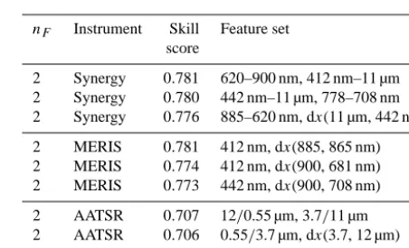
Table 1. Best found results for feature sets of classical Bayesian cloud masks with two strongly independent features which best recreate Synergy cloud mask results. The results are separated for the Synergy of MERIS and AATSR, MERIS, and AATSR. Chan-nels are referenced by their central wavelength. MERIS chanChan-nels use the unit nm, while AATSR channels use µm.
nF Instrument Skill Feature set
score
2 Synergy 0.781 620–900 nm, 412 nm–11 µm 2 Synergy 0.780 442 nm–11 µm, 778–708 nm 2 Synergy 0.776 885–620 nm, dx(11 µm, 442 nm)
2 MERIS 0.781 412 nm, dx(885, 865 nm) 2 MERIS 0.774 412 nm, dx(900, 681 nm) 2 MERIS 0.773 442 nm, dx(900, 708 nm)
2 AATSR 0.707 12/0.55 µm, 3.7/11 µm 2 AATSR 0.706 0.55/3.7 µm, dx(3.7, 12 µm) 2 AATSR 0.706 0.55/12 µm, dx(12, 3.7 µm)
after crossing the blue line vs. number of points before cross-ing) are quite similar. Figure 7 shows that the Bayesian cloud mask with four features exhibits a much smoother distribu-tion of probabilities and a decreased rate of misses, while the improvement of the false alarm rate is only minor. Also, the impact of changing the threshold value can be nicely seen. The overall skill score seems to be almost unaffected when changing the threshold. The false alarm rate decreases when the threshold is increased, but at the same time the rate of misses increases, which would decrease the skill score.
Table 2. Similar to Table 1 but for classical Bayesian cloud masks based on four strongly independent features.
nF Instrument Skill Feature set score
4 Synergy 0.826 1.6 µm, 681/778 nm, dx(0.55 µm, 760 nm), dx(11 µm, 412 nm) 4 Synergy 0.821 412 nm, 12 µm, 753 nm×1.6 µm, dx(11, 12 µm)
4 Synergy 0.820 442 nm, 3.7–11 µm, 3.7 µm×12 µm, dx(665, 753 nm)
4 MERIS 0.822 412 nm, 900 nm×510 nm, dx(760, 620 nm), dx(885, 865 nm)
4 MERIS 0.821 753/510 nm, 442 nm×412 nm, dx(865, 753 nm), dx(885, 760 nm)
4 MERIS 0.818 442, 665/900 nm, dx(560, 510 nm), dx(865, 885 nm)
4 AATSR 0.765 12, 0.55 µm, 12/3.7 µm, 0.55/0.87 µm
4 AATSR 0.757 0.67 µm, 12/3.7 µm, 0.87/0.55 µm, 11/0.67 µm
4 AATSR 0.757 0.55/0.87 µm, 12 µm×3.7 µm, dx(0.55, 3.7 µm), dx(12, 11 µm)
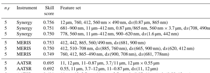
Table 3. Similar to Table 3 but for naive Bayesian cloud masks based on five strongly independent features.
nF Instrument Skill Feature set score
5 Synergy 0.756 12 µm, 760, 412, 560 nm×490 nm, dx(0.87 µm, 865 nm)
5 Synergy 0.751 681–900 nm, 11 µm–412 nm, 0.87 µm/865 nm, 560 nm×3.7 µm, dx(708, 490nm) 5 Synergy 0.750 778, 560 nm, 11 µm–412 nm, 900–620 nm, dx(1.6 µm, 442 nm)
5 MERIS 0.753 412, 442, 865, 560/490 nm, dx(681, 900 nm)
5 MERIS 0.750 412, 510–708 nm, dx(885, 760 nm), dx(665, 900 nm), dx(620, 412 nm)
5 MERIS 0.749 760, 412, 865–490 nm, dx(900, 708 nm), dx(681, 778nm)
5 AATSR 0.695 11, 12 µm, 11–0.87 µm, 3.7/11 µm, 12 µm×0.55 µm
5 AATSR 0.692 0.55, 11 µm, 3.7–12 µm, 11–0.87 µm, dx(11, 12 µm)
5 AATSR 0.691 11 µm, 12–3.7 µm, 11 µm×3.7 µm, dx(0.87, 11 µm), dx(0.55, 12 µm)
alone is used. The results for AATSR alone are significantly inferior. For the Synergy data set, the 11 µm channel in com-bination with a MERIS channel in the blue (412 and 442nm) is found in all three top results. For MERIS alone, a com-bination of a channel in the blue and an index of red and short-wave infrared channels is found in the top results. It is quite counterintuitive that the best results for MERIS are achieved with only three different channels, while the algo-rithm had the freedom to select up to four channels. The best result for the set of Synergy channels included four channels, which relates more to the naive intuition that more channels carry more information and would therefore be better suited for the application. However, since the search space was not fully covered, a better solution for MERIS with four channels could still be found.
Table 2 shows similar results but for classical Bayesian cloud masks based on a set of four features. Again, Synergy and MERIS results are significantly better than those from AATSR, while the Synergy results are only slightly better then those from MERIS alone. All possible feature functions are used within the results but of course not all the time for any result.
Similar studies were also performed for higher numbers of features, but no results with significantly higher skill scores were found. The skill score results for using three features are positioned right in the middle of the two discussed re-sults, such that four features seems to be the best choice to reproduce the Synergy cloud mask with a classical Bayesian cloud mask based on strongly independent features.
Similar searches for naive Bayesian cloud masks with strongly independent features were performed for 5 and 15 features, and results for five features are shown in Table 3. The search with 15 features did not show significantly bet-ter result than the ones shown. In general, these results are not as successful in reproducing the Synergy cloud mask as the approaches with the classical Bayesian cloud mask. Skill scores for AATSR alone are smaller than for MERIS and Synergy and also generally smaller than for the classical ap-proach with four features.
0% 10% 20% 30% 40% 50% 60% 70% 80% 90% 100%
fraction of total cases
0.0
0.2
0.4
0.6
0.8
1.0
Baysian cloud probability
P(C,FA), for SYN(cloudy)
P(C,FA), for SYN(cloud free)
P(C,FB), for SYN(cloudy)
P(C,FB), for SYN(cloud free)
Figure 7. Cloud probability from the two classical Bayesian cloud masks from Fig. 5 (dashed line,P (C,FA)) and Fig. 6 (solid line, P (C,FB)) separated by cases which were labeled as cloudy (red) and non-cloudy (green) by the Synergy cloud mask. The same data as in Figs. 5 and 6 were used and the results were sorted for a better overview. The threshold of 0.5 cloud probability is marked with a blue line.
skill score can be achieved with many different feature sets. From a technical point, it is then sufficient to choose one of those results with best skill scores, even if this might not be the absolute global maximum.
Some commonly used features, such as the brightness tem-perature difference of 11 and 12 µm, did not appear in the shown results. However, this does not indicate that the found features are in general superior to those missing. It simply states that during the search no set of features were found which included them and shows better results. Restricting the search space to cover only selected features is simple and could be used to limit the results to features with known physical meaning.
For both classical and naive Bayesian cloud masks, a spe-cific set of features should be evaluated as a whole. The effect of a certain feature on the skill score for the total feature set can be estimated by evaluating results for a particular set with and without the feature in question. The effect on the skill score when adding a feature to a given set might strongly de-pend on the original feature set. In addition, features which show only poor reproduction skill when used alone might significantly improve the skill score for a certain set of fea-tures.
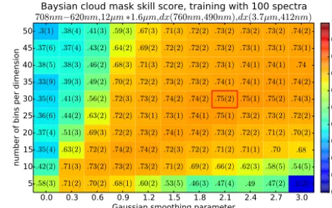
Next, the impact of the number of bins nB, Gaussian smoothing value, and sample size of the artificial truth data set is discussed. The sensitivity of the Bayesian cloud mask in terms of skill score with respect to a certain feature set is shown in Figs. 8 and 9. Both figures show skill scores for Synergy cloud mask artificial truth data with respect to number of bins, Gaussian smoothing factor, and sample size of the artificial truth data. Figure 8 shows an extreme case where only 100 randomly selected globally distributed cases were used as artificial truth. Again, the year 2007 was used as
0.0 0.3 0.6 0.9 1.2 1.5 1.8 2.1 2.4 2.7 3.0 Gaussian smoothing parameter
5 10 15 20 25 30 35 40 45 50
number of bins per dimension
.58(3) .71(2) .70(2) .68(1) .60(2) .53(5) .46(3).47(4) .49 .47(2) .1(2)
.42(2) .71(3) .73(2) .73(2) .73(2) .71(2) .69(2).66(2).62(3).58(5) .54(5)
.35(4) .63(2) .72(2) .74(2) .74(2) .72(3) .72(2).71(2).71(1) .70 .68
.37(4) .51(3) .69(3) .72(2) .73(2) .74(1) .74(2).73(2).72(2).71(2) .70(2)
.36(6) .44(2) .63(2) .72(2) .73(1) .73(1) .74(1).75(1).73(2).73(2) .72(2)
.35(6) .41(3) .56(2) .72(3) .73(2) .74(2) .74(2).75(2).75(1).75(2) .74(3)
.33(9) .39(3) .49(2) .70(2) .72(2) .73(2) .73(2).74(1).74(1).74(1) .74(2)
.38(5) .38(3) .46(2) .68(3) .71(3) .72(2) .73(2).73(1).74(1).74(1) .74
.37(6) .37(4) .43(2) .64(2) .69(2) .72(2) .72(2).73(2).73(1).73(1) .73(1)
.3(1) .38(4) .41(3) .59(3) .67(3) .71(3) .72(2).73(2).73(2).73(2) .74(2)
Baysian cloud mask skill score, training with 100 spectra
708nm−620nm,12µm∗1.6µm,dx(760nm,490nm),dx(3.7µm,412nm)
0.0 0.1 0.2 0.3 0.4 0.5 0.6 0.7 0.8 0.9 1.0
Hansen Kuipers skill score
Figure 8. Skill score of a classical Bayesian cloud mask with four strongly independent features with respect to number of bins for each dimension of the underlying histograms and the applied Gaus-sian smoothing. Artificial truth data are taken from 2007 and skill scores were computed for the year 2008. Only 100 randomly se-lected and globally distributed spectra were used to compute the histograms. This selection was repeated 10 times and mean values for the skill score are shown. The standard deviation on the last sig-nificant digit is shown in parenthesis.
pool for the artificial truth and the year 2008 to compute the skill score. The skill scores of the cloud mask which is based on such a small sample size clearly depends on the sample itself. The procedure was repeated 10 times and the achieved mean skill score is shown. The standard deviation in the last digit is shown in parenthesis.
With no Gaussian smoothing applied, the skill score clearly decreases with increasing number of bins since the sample size is much too small for this resolution. Also, the impact of the sample is largest when the standard deviation is highest. The skill score increases with increasing number of bins and Gaussian smoothing until a maximum is reached. With the increasing bin number and smoothing, the skill score decreases only slightly. In this case, an optimal set of bin size and smoothing can be found. When smaller vales are used, the skill scores are drastically reduced, but when larger values are used, the skill score decreases only slightly.
A similar sensitivity study is shown in Fig. 9, but here a much larger sample size of artificial truth data was used. Again, without Gaussian smoothing the smallest number of bins shows the best results, while with increasing number of bins the skill score decreased because the total number of bins grows with the fourth potential of the number of bins. A large plateau of consistently stable and high skill score values is found for numbers of bins above 25 and Gaussian smoothing above 0.9.
0.0 0.3 0.6 0.9 1.2 1.5 1.8 2.1 2.4 2.7 3.0 Gaussian smoothing parameter
5 10 15 20 25 30 35 40 45 50
number of bins per dimension
.79 .79 .76 .70 .66 .52 .46 .43(1) .46 .46(3) .53(2)
.81 .81 .81 .79 .77 .75 .72 .69 .64 .61 .56
.81 .82 .82 .81 .80 .79 .77 .76 .74 .72 .70
.79 .82 .83 .82 .82 .81 .80 .79 .77 .76 .75
.75 .81 .83 .83 .82 .82 .81 .80 .79 .78 .77
.70 .80 .83 .83 .83 .82 .82 .81 .80 .80 .79
.64 .80 .82 .83 .83 .83 .82 .82 .81 .81 .80
.58 .79 .82 .83 .83 .83 .83 .82 .82 .81 .81
.54 .79 .82 .83 .83 .83 .83 .83 .82 .82 .81
.50 .78 .81 .83 .83 .83 .83 .83 .82 .82 .82
Baysian cloud mask skill score, training with 100000 spectra
708nm−620nm,12µm∗1.6µm,dx(760nm,490nm),dx(3.7µm,412nm)
0.0 0.1 0.2 0.3 0.4 0.5 0.6 0.7 0.8 0.9 1.0
Hansen Kuipers skill score
Figure 9. Similar to Fig. 8 but the sample size of the artificial truth was 1000 times larger with 100 k cases.
information in incomplete histograms such that it better rep-resents the true probability density.
In general, one can not perform such studies to assess the optimal number of bins and value of Gaussian smoothing parameter, because only an insufficient number of artificial truth data might be available. The presented results from nu-merical experiments indicate that for four features and a suf-ficiently large sample of artificial truth data, a bin size of 40 with a Gaussian smoothing of 1.5 is a good choice. This result holds not only for the presented feature set but also for many other sets which have been assessed during this re-search.
7.2 Enhancements of existing algorithms
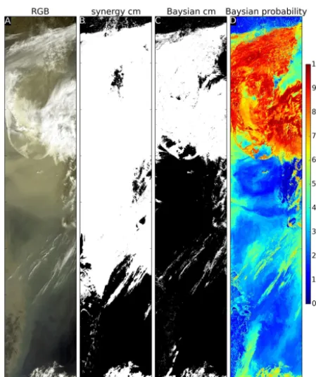
It was shown so far that Bayesian cloud masks can be used to reproduce at least one existing cloud mask up to a certain extent. It is unclear, however, what the limiting factors are in global skill score with respect to this particular cloud mask. A major contributor to this upper limit can be inconsistencies in the artificial truth data set. Examples are shown in panel a and b of Figs. 10 and 11, which actually show the surround-ings of the scenes shown in Figs. 1 and 2. Both figures show some classification errors of the Synergy cloud mask. The top part of Fig. 10 shows a partly cloudy scene over a large ice-or snow-covered area which is completely masked as cloudy (white areas in panel b). In addition, the arrow-shaped land area in the lower part of the figure (Brodeur Peninsula on Baffin Island) is clearly not cloudy but is classified as cloudy. Similarly in Fig. 11, the complete dust storm east of the Ko-rean peninsula is marked as cloudy. Such classification er-rors introduce inconsistencies which affect the produced his-tograms and are in general difficult to reproduce with an in-dependent system.
The appearance of such errors does not mean that the algo-rithm should be abandoned and with it all the work that has been invested into developing it. Panels c and d in Figs. 10 and 11 show how the Bayesian cloud mask technique can be
Figure 10. (a) shows an RGB view of a larger area of the scene which is shown in Fig. 1. (b) shows results of the non-Bayesian Synergy cloud mask with some classification errors over the top snow and ice region and the arrow-shaped land area in the bottom of the figure. (c) shows results of a Bayesian cloud mask which is based on corrected artificial truth from this scene and the one shown in Fig. 11. (c) shows the cloud probability results of this Bayesian cloud mask.
used to enhance this existing algorithm when errors in the artificial truth data are manually corrected by an human ex-pert. Synergy cloud mask results from these two orbits were manually corrected and used as artificial truth to produce a classical Bayesian cloud mask based on four strongly inde-pendent features. The two orbits were then reprocessed and the resulting cloud masks and cloud probabilities are shown. Some artifacts at land and ice boundaries are still present, but the major classification errors were strongly reduced.
Figure 11. Similar to Fig. 10 but a larger area corresponding to Fig. 2 is shown. (b) shows results of the non-Bayesian Synergy cloud mask where the strong dust storm is completely classified as cloud. (c) shows results of a Bayesian cloud mask which is based on corrected artificial truth from this scene and the one shown in Fig. 10. (c) shows the cloud probability results of this Bayesian cloud mask.
data gaps, or better representativity gaps, can then be filled with artificial truth data from manual classification. Such an approach can be used to focus the attention of the human ex-perts to areas where their expertise is most strongly needed and to use their available labor in the most efficient way.
As discussed in Sect. 7.1, possibly many different fea-ture sets can be used to recreate the algorithms which were used to produce the artificial truth data. This property can be used to produce much more robust cloud masking algo-rithms. When the seeding algorithm cannot cope with miss-ing data when, e.g., a certain needed channel is flagged as unusable or saturated, one can simply switch to a different Bayesian cloud mask which does not depend on that chan-nel. The operational version of the cloud mask for the Cloud CCI project contains several ranked Bayesian cloud masks, and when the top mask fails to produce a result, a mask of lower rank is used until the last mask is used or the algo-rithm produces a result. This approach can greatly reduce the number of unprocessed measurements for a cloud masking scheme.
7.3 Cloud masks from manually classified data
Human experts can produce artificial truth data of high qual-ity by careful manual classification of MERIS, AATSR, or Synergy images. It is of great advantage that the spatial res-olution of MERIS and AATSR images is high enough that spatial and spectral patterns together can be used to clas-sify data points. Cloud shadows, for instance, can be used to clearly distinguish clouds from snow and ice surfaces. In that respect, the algorithm itself is not based on spatial informa-tion, but it was surely used to create the artificial truth data. It is beyond the scope of this paper to produce a cloud mask with global applicability, but it should be demonstrated how straightforward such a procedure would be. The results pre-sented here are then clearly applicable to OLCI and SLSTR on-board the upcoming Sentinel-3 satellite.
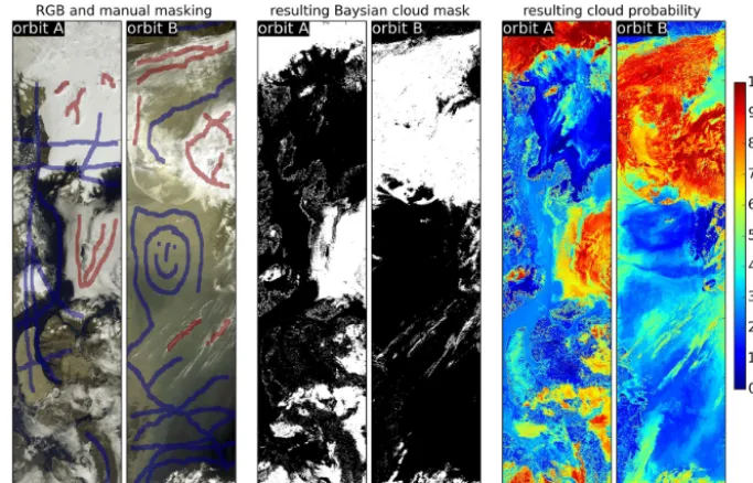
The same two orbits which were discussed in Sects. 4 and 7.2 are used for the procedure. Both orbits contain scenes which are in general difficult to classify accurately, such as clouds over a and ice-covered region, cloud-free snow-and ice-covered surfaces, or a pronounced dust storm. The manual classification setup was designed such that no spe-cial computational knowledge is needed to perform the cloud classification. For each test orbit, image files containing sev-eral layers were created. The various image layers include an RGB image, contrast stretched gray-scale images from Synergy channels, and several feature functions which were found to be of good performance in the Bayesian framework. To classify actual pixels, the human expert has to color ar-eas (e.g., blue color for cloud free and red color for cloudy) in a blank image layer. By adjusting the transparency of the single layers, each scene can be carefully inspected before a decision is made. The actual shape of the colored areas is of lower importance as well as the actual number of classi-fied areas. However, the total variability of possible cases and scenes should be included in the classification.
Results of this procedure are shown in Fig. 12. The left-most two panels show an RGB view of the scene and with blue and red color the areas which were classified by the hu-man expert. The actual number of the classified area is small compared to the total size of the scene. Then, this data set was used as artificial truth and a classical Bayesian cloud mask with four strongly independent features was set up to process the two orbits. The resulting cloud masks are shown in the middle two panels, while the actual cloud probability is shown in the two rightmost panels.
Figure 12. Manual classifications of the scenes shown in Figs. 1 and 2. Shown are the cloudy and non-cloudy classification together with an RGB view for two scenes (two leftmost panels, blue is non-cloudy, red is cloudy), the resulting cloud mask (two middle panels), and the cloud probability (rightmost two panels).
the artificial truth data set and as self-describing documenta-tion of the algorithm.
This approach is most straightforward when the spatial resolution of the instrument in question is high enough that the human expert can use the spatial pattern information to correctly classify cloudy from non-cloudy areas. For global applicability, a higher number of orbits with representative spatial and seasonal sampling should be included in the set of considered artificial truth data. Especially complex cases such as scenes with ice, snow, sun glint, mountains, or dust storms should be included in the classification effort.
8 Conclusions
The application of the classical and naive Bayesian cloud masking technique to MERIS, AATSR, and their Synergy was discussed in detail. Bayesian cloud masks based on in-dependent features are numerically highly efficient and are very well suited for the fast processing of large numbers of data. This technique will be applied to a reprocessing of the 9.5 year time series of MERIS and AATSR measurements within ESA’s Cloud CCI project.
Details of the actual implementation of the Bayesian cloud mask for Cloud CCI are not part of this paper. The algo-rithm is implemented in Python and is based on the multi-processing, SciPy, and NumPy libraries (van der Walt et al., 2011). Effective parallelization is achieved trough separa-tion of CPU bound and input / output (I /O) tasks. Process-ing time per orbit is largely dominated by I /Oand the ac-tual time spend in the Bayesian scheme is 1 order of
magni-tude smaller than the total run time. Currently, the scheme supports the classical and naive approach for independent Bayesian cloud masks. The final set of features for process-ing the complete Cloud CCI period of 9.5 years will be de-termined in the near future before starting the generation of level 3 data.
Sufficient numbers of artificial truth data and the frequen-tist approach can be used to estimate multidimensional his-tograms for the estimation of background joint probabili-ties. Gaussian smoothing of appropriate width can be used to drastically reduce the actual numbers of truth data needed to compute histograms for the classical Bayesian approach. This post-processing step greatly simplifies our ability to fur-ther explore the classical Bayesian approach.
Due to restrictions of modern computer hardware, the practical limit for the classical Bayesian approach is reached with six to seven features. This does not actually restrict its applicability, since trivial feature functions can be used which combine any number of measurements into a single feature.
to be present in the best results when the set of selected fea-ture functions and channels was numerically optimized.
The broad spectral range and the number of available channels within the Synergy data set can be used to set up Bayesian cloud masks with very similar classification skill but based on different combinations of channels. This can be used to design cloud masking schemes which are robust against partially missing data.
It was shown how Bayesian cloud masks can be used to reproduce the results of existing algorithms, improve exist-ing algorithms and how to set up new classification schemes based on manual classification by human experts. Reproduc-ing existReproduc-ing algorithms offers the perspective of increased numerical efficiency and processing robustness. The ap-proach based on manual image classification is straightfor-ward for the human expert. Classified scenes can be stored and revisited if the produced cloud masks show misclassifi-cations in certain areas or weather conditions. When errors are not traceable to errors in the manual classification, addi-tional scenes can be added to the set of artificial truth data to increase the chance of correct classification.
The presented results for MERIS and AATSR can be used to implement an accurate and highly efficient cloud masking scheme for OLCI and SLSTR on-board the upcoming Sen-tinel 3 satellite. Especially the additional oxygen absorption channels from the OLCI instrument might be used within an improved and numerically efficient cloud classification algo-rithm.
Although this paper is focused on strongly independent Bayesian cloud masks, there is no apparent reason which prevents the application of the introduced techniques to the case of dependent Bayesian cloud masks. It is straightfor-ward to include external information such as clear sky radi-ance estimators or NWP fields in the proposed optimization strategy for the construction of features. The application of Gaussian smoothing to derived histogram fields is indepen-dent of external information and can be used to reduce the numbers of needed truth data. To actually assess the added value of the external data, one must assure that the quality of the truth data is sufficient. In the case of MERIS and AATSR, one likely needs a reasonable large set of manually classified data.
Acknowledgements. This work has been funded by the European
Space Agency in the framework of the Climate Change Initiative project and by the German Federal Ministry of Education and Research (BMBF) in the framework of the HD(CP)2project.
Edited by: A. Kokhanovsky
References
Carbajal Henken, C. K., Lindstrot, R., Preusker, R., and Fischer, J.: FAME-C: cloud property retrieval using synergistic AATSR
and MERIS observations, Atmos. Meas. Tech. Discuss., 7, 4909– 4947, doi:10.5194/amtd-7-4909-2014, 2014.
Coppo, P., Ricciarelli, B., Brandani, F., Delderfield, J., Ferlet, M., Mutlow, C., Munro, G., Nightingale, T., Smith, D., Bianchi, S., Nicol, P., Kirschstein, S., Hennig, T., Engel, W., Frerick, J., and Nieke, J.: SLSTR: a high accuracy dual scan temperature ra-diometer for sea and land surface monitoring from space, J. Mod. Optic., 57, 1815–1830, doi:10.1080/09500340.2010.503010, 2010.
English, S., Eyre, J., and Smith, J.: A cloud-detection scheme for use with satellite sounding radiances in the context of data as-similation for numerical weather prediction, Q. J. Roy. Meteor. Soc., 125, 2359–2378, 1999.
Fomferra, N. and Brockmann, C.: Beam-the ENVISAT MERIS and AATSR toolbox, in: MERIS (A)ATSR Workshop 2005, 597, p. 13, 2005.
Gómez-Chova, L., Camps-Valls, G., Amorós-López, J., Guanter, L., Alonso, L., Calpe, J., and Moreno, J.: New cloud detection algo-rithm for multispectral and hyperspectral images: Application to ENVISAT/MERIS and PROBA/CHRIS sensors, in: IEEE Inter-national Geoscience and Remote Sensing Symposium, IGARSS, 2757–2760, 2006.
Gómez-Chova, L., Camps-Valls, G., Munoz-Marı, J., Calpe, J., and Moreno, J.: Cloud screening methodology for MERIS/AATSR Synergy products, in: Proc. 2nd MERIS/AATSR User Workshop, ESRIN, Frascati, 22–26, 2008.
Hall, D. K., Riggs, G. A., Salomonson, V. V., DiGirolamo, N. E., and Bayr, K. J.: MODIS snow-cover products, Remote Sens. En-viron., 83, 181–194, 2002.
Hanssen, A. W. and Kuipers, W. J. A.: On the Relationship Be-tween the Frequency of Rain and Various Meteorological Param-eters: (with Reference to the Problem of Objective Forecasting), Staatsdrukkerij-en Uitgeverijbedrijf, 1965.
Heidinger, A. K., Evan, A. T., Foster, M. J., and Walther, A.: A naive Bayesian cloud-detection scheme derived from CALIPSO and applied within PATMOS-x, J. Appl. Meteorol. Clim., 51, 1129– 1144, 2012.
Hollmann, R. and Lecomte, D. P.: Climate Assessment
Report, Tech. rep., ESA Cloud CCI, available at:
http://www.esa-cloud-cci.org/sites/default/files/documents/ public/Cloud_CCI_D4-2_CAR_1.0.pdf (last access: 13 April 2015), 2013.
Hollmann, R., Merchant, C., Saunders, R., Downy, C., Buchwitz, M., Cazenave, A., Chuvieco, E., Defourny, P., De Leeuw, G., Forsberg, R., Holzer-Popp, T., Paul, F., Sandven, S., Sathyen-dranath, S., and Roozendael, M.: The ESA climate change initia-tive: Satellite data records for essential climate variables, B. Am. Meteorol. Soc., 94, 1541–1552, 2013.
Kriegler, F., Malila, W., Nalepka, R., and Richardson, W.: Prepro-cessing transformations and their effects on multispectral recog-nition, in: Remote Sens. Environ., VI, vol. 1, p. 97, 1969. Llewellyn-Jones, D., Edwards, M., Mutlow, C., Birks, A., Barton,
I., and Tait, H.: AATSR: Global-change and surface-temperature measurements from Envisat, ESA bulletin, 105, 11–21, 2001. Mackie, S., Embury, O., Old, C., Merchant, C., and Francis, P.:
Mackie, S., Merchant, C., Embury, O., and Francis, P.: Generalized Bayesian cloud detection for satellite imagery. Part 2: Technique and validation for daytime imagery, Int. J. Remote Sens., 31, 2595–2621, 2010b.
Merchant, C., Harris, A., Maturi, E., and MacCallum, S.: Proba-bilistic physically based cloud screening of satellite infrared im-agery for operational sea surface temperature retrieval, Q. J. Roy. Meteor. Soc., 131, 2735–2755, 2005.
Miguel, A., Bruno, B., Jean-Loup, B., Mark, D., Florence, H., Ulf, K., Constantinos, M., Pierluigi, S., Bruno, G., and Jerome, B.: Sentinel-3 – the ocean and medium-resolution land mission for GMES operational services, ESA Bulletin (ISSN 0376-4265), 131, 24–29, 2007.
Murtagh, F., Barreto, D., and Marcello, J.: Decision boundaries us-ing Bayes factors: the case of cloud masks, IEEE T. Geosci. Re-mote, 41, 2952–2958, 2003.
Nieke, J.: Status of the optical payload and processor development of ESA’s Sentinel 3 mission, Geoscience and Remote Sensing Symposium, 2008, IGARSS 2008, IEEE International, 4, 427– 430, 2008.
Rast, M., Bezy, J. L., and Bruzzi, S.: The ESA Medium Res-olution Imaging Spectrometer MERIS a review of the instru-ment and its mission, Int. J. Remote Sens., 20, 1681–1702, doi:10.1080/014311699212416, 1999.
Rossow, W. B. and Garder, L. C.: Cloud detection using satellite measurements of infrared and visible radiances for ISCCP, J. Cli-mate, 6, 2341–2369, 1993.
Schlundt, C., Kokhanovsky, A. A., von Hoyningen-Huene, W., Din-ter, T., Istomina, L., and Burrows, J. P.: Synergetic cloud fraction determination for SCIAMACHY using MERIS, Atmos. Meas. Tech., 4, 319–337, doi:10.5194/amt-4-319-2011, 2011. Stubenrauch, C., Rossow, W., Kinne, S., Ackerman, S., Cesana, G.,
Chepfer, H., and Di, L.: Assessment of Global Cloud Data Sets from Satellites, A Project of the World Climate Research Pro-gramme Global Energy and Water Cycle Experiment (GEWEX) Radiation Panel, 2012.
Uddstrom, M. J., Gray, W. R., Murphy, R., Oien, N. A., and Murray, T.: A Bayesian cloud mask for sea surface temperature retrieval, J. Atmos. Ocean. Tech., 16, 117–132, 1999.
van der Walt, S., Colbert, S., and Varoquaux, G.: The NumPy Array: A Structure for Efficient Numerical Computation, Comput. Sci. Eng., 13, 22–30, doi:10.1109/MCSE.2011.37, 2011.