www.ocean-sci.net/7/175/2011/ doi:10.5194/os-7-175-2011
© Author(s) 2011. CC Attribution 3.0 License.
Ocean Science
A global comparison of Argo and satellite altimetry observations
A. -L. Dhomps1, S. Guinehut1, P.-Y. Le Traon2, and G. Larnicol1 1CLS, Space Oceanography Division, Ramonville Saint-Agne, France 2Ifremer, Technopole de Brest-Iroise, Plouzan´e, France
Received: 30 April 2010 – Published in Ocean Sci. Discuss.: 12 May 2010 Revised: 31 January 2011 – Accepted: 1 March 2011 – Published: 10 March 2011
Abstract. Differences, similarities and complementarities between Sea Level Anomalies (SLA) deduced from altimeter measurements and dynamic height anomalies (DHA) calcu-lated from Argo in situ temperature (T) and salinity (S) pro-files are globally analyzed. SLA and DHA agree remarkably well and, compared to previous studies, Argo dataset allows an improvement in the coherence between SLA and DHA. Indeed, Argo data provides a much better spatial coverage of all oceans and particularly the Southern Ocean, the use of an Argo mean dynamic height, the use of measured salinity pro-files (versus climatological salinity), and the use of a deeper reference level (1000 m versus 700 m). The large influence of Argo salinity observations on the consistency between al-timetry and hydrographic observations is particularly demon-strated with an improvement of 35% (relative to the SLA mi-nus DHA signal) by using measured salinity profiles instead of climatological data. The availability of observations along the Argo float trajectories also provides a means to describe the sea level variability of the global ocean both for the low frequency and the mesoscale part of the circulation. Results indicate that sea level variability is dominated by baroclinic signal at seasonal to inter-annual periods for all latitudes. In the tropics, sea level variability is baroclinic for meso-scale to interannual periods and at high latitudes, sea level vari-ability is barotropic with also deep baroclinic signals (i.e. influence of deep temperature and salinity signals) for intra seasonal and mesoscale periods. These results emphasize the need to separate the different time and space scales in order to improve the merging of the two data sets. The qualita-tive study of seasonal to interannual SLA minus DHA sig-nals finally reveals sigsig-nals related to deep ocean circulation variations and basin-scale barotropic signals. Future work is, however, needed to understand the observed differences and relate them to different forcing mechanisms.
Correspondence to: A.-L. Dhomps ([email protected])
1 Introduction
In November 2007, the global Argo array of profiling floats reached its initial target of 3000 operating floats worldwide. The array provides for the first time a global monitoring of ocean temperature and salinity data in real time (Roemmich et al., 2009). In the meantime, satellite altimeters continue to provide global and synoptic measurements of sea level vari-ations. These observations are now the two most important and complementary components of the global ocean observ-ing system required by climate and operational oceanogra-phy applications (Bell et al., 2009). The study of their con-sistency is an essential step before the data are jointly assim-ilated in ocean general circulation models.
Differences, similarities and complementarities between Sea Level Anomalies (SLA) deduced from altimeter mea-surements and dynamic height anomalies (DHA) calculated from in situ temperature (T) and salinity (S) profiles have al-ready been studied globally by (Guinehut et al., 2006; here-after referred to as GLL06). As SLA reveal both barotropic and baroclinic component of the ocean circulation, DHA, calculated with in situ temperature and salinity, reveal only the baroclinic part of the ocean circulation between the sur-face and a chosen reference level. In GLL06, authors showed very good correlation between the two data sets but also systematic large-scale differences that have been related to a barotropic, Sverdrup-like, response of the ocean to wind forcing. This previous study, focused on the 1993–2003 pe-riod, was limited by the in situ observations available. In-deed, at that time, the in situ dataset was mainly composed of XBT instruments. The GLL06 study is revisited here using the new available Argo data set. The Argo data set allows a series of improvements ranging from: (1) a better global spatial coverage (i.e. Southern Ocean), (2) a deeper refer-ence level (1000 m versus 700 m), (3) the use of measuredS
The full Argo dataset was downloaded from the Coriolis Global Data Acquisition Center as of September 2008 for the 2001–2007 periods and as of January 2009 for the year 2008 (http://www.coriolis.eu.org). The dataset went through the real-time quality control procedures applied by each Data Acquisition Center and about half of the profiles older than one year have went through delayed-mode procedures (see the Argo quality control manual for more details: Wong et al., 2008). For this study, when available, adjusted fields (delayed-mode and real-time) are preferred to real-time ones and only measurements having pressure, temperature, and salinity observations considered “good” (i.e. with a quality flag numerical grade of “1”) are used. In the GLL06 study, the reference level for the analyses was chosen at 700 m be-cause the in situ observations were mainly composed of XBT instruments. 350 000 700 m depth profiles were used for the 1993–2003 period because only 90 000 1000 m depth profiles were available. With the Argo dataset, it is possible to deepen the reference level to 1000 m. A total of 325 650 1000 m depth validated profiles are collected for the 2001–2008 pe-riod. As many floats do not profile deeper than 1000 m at low latitudes due to technical limitations, a 1500 m reference level reduces the number of profiles to 230 200 but mainly involves an under-sampling of the tropical oceans. Using a 1000 m reference level reduces slightly the number of pro-files compared to the previous study but improves the spatial coverage of the analyses.
Measured S profiles were not available for the GLL06 study as the in situ observations came mainly from XBT instruments. To analyze the impact of Argo measured S, a climatological salinity profile has been interpolated for each Argo profile. As in GLL06, the method uses a sim-ple salinity-depth relationship as a function of the geograph-ical position and using the World Ocean Atlas 2005 monthly fields (WOA05: Antonov et al., 2006; Locarnini et al., 2006). Impact of measured and climatological salinity on DHA/SLA consistency can then be studied.
The altimeter data used are delayed-mode fields of SLA obtained from an optimal combination of all available satel-lite altimeters that are distributed by AVISO (AVISO, 2010). The fields are available every 7 days on a Mercator grid of 1/3◦resolution at the equator. As this product provides SLA
Finally, SLA maps are interpolated to the time and location of each in situ DHA measurement using a linear space/time interpolation.
3 Correlation between Argo and altimeter observations
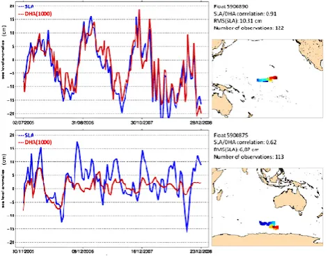
Correlation coefficients between all collocated SLA and DHA time series were first calculated on a 1◦×1◦horizontal grid using observations available in a 5◦longitude by 2◦ lati-tude box of influence around each grid point (Fig. 1b). These parameters have been chosen in order to reduce the prob-lems due to the non-uniform temporal and spatial distribution of in situ measurements, to take into account the latitudinal structure of the correlation signal and to obtain a relatively large-scale uniform map. Besides, the relatively large-scale size of the box smoothes the small-scales signals and leads to global interpretations. Correlation coefficients show val-ues greater than 0.8 in most part of the Indian and Pacific oceans. The Southern Oceans and the northern part of the North Atlantic Ocean show, as expected, lower values, in the order of 0.6 or less. This can be explained by the influence of deep baroclinic and barotropic signals in these regions. Three tropical sub-regions also show lower values of the same or-der: the South East Pacific Ocean and the South and North Tropical Atlantic Ocean. These regions correspond to areas where the sea level and steric sea level variabilities are very small (<3 cms rms) as well as the signal to noise ration. Thus high correlations are difficult to obtain between them. As an example, collocated SLA/DHA observations are showed on Fig. 2 for two Argo floats. In the Equatorial Pacific, SLA and DHA signals are very similar with high correlation (0.91). In the Southern Ocean, DHA have smaller amplitude than SLA and the correlation is smaller (0.62).
Fig. 1. Correlation coefficients (b) and regression coefficients (c) between SLA and DHA. The mean correlation as a function of lati-tude is also represented (a).
Fig. 2. DHA and collocated SLA for two Argo floats. The position of each float are also indicated, the blue cross corresponding to the deployment position, and the red cross to its last position.
values of the regression coefficients at high latitudes are due to strong barotropic signal and deep baroclinic signals (Vino-gradova et al., 2007). This leads to an underestimation of the steric part of the sea level by DHA calculated using a 1000 m depth reference level (Fig. 1c). Additionally, the regression coefficients are also useful to calculate DHA from SLA ob-servations and to derive the 3-D ocean state from SLA obser-vations through data assimilation.
Additionally to correlation coefficients and regression co-efficients, variances of SLA and DHA, both calculated on a 1◦×1◦ grid, display very similar patterns with very close amplitudes, showing again the very good consistency
Fig. 3. Rms of SLA (a), of DHA (b) and of the differences (SLA-DHA) when DHA are calculated from ArgoT/Sprofiles (c) and of the differences (SLA-DHA) when DHA are calculated from Argo
T profiles andSprofiles from the WOA05 climatology (d).
between Argo and altimeter observations (Fig. 3a and b). However and as expected, DHA variance shows lower ampli-tudes in the Brazil-Malvinas Confluence region and Antarc-tic Circumpolar Current (ACC) regions where eddies deeper than 1000 m depth are found.
Given the higher number of observations available in each 5◦ longitude by 2◦latitude radius of influence around each grid point (>500), the 95% confidence interval is of the order of 0.05 for the correlation coefficient, 0.07 for the regression coefficient and almost everywhere smaller than 1 cm rms for the variance fields. These numbers increase up to 0.1 for the correlation coefficient and 0.15 for the regression coefficient in the three tropical sub-regions mentioned above and south of 55◦S where the number of observations decrease to 100 or less. Error associated to each global statistic given later on in the paper are much smaller and of the order of 0.001 for the correlation coefficient and of the order of 0.01 cm rms for the variance due to the 325 000 validated profiles used. All the results given thereafter are thus highly significant in the 95% confidence interval.
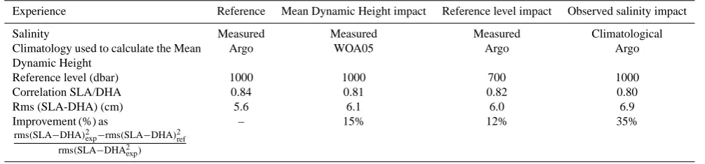
It is worth highlighting that the Argo mean dynamic height already provides improved comparison between SLA and DHA compared to the use of a climatological mean dynamic height. The rms difference between SLA and DHA is re-duced to 5.6 cm rms when using the Argo mean dynamic height from 6.1 cm rms when the WOA05 is used. This cor-responds to an improvement of 15% of the variance in the consistency of the two datasets (see Table 1). Their global correlation is also increased from 0.81 to 0.84. This is mainly the result of the reduction of the mean global bias of 1.0 cm that exists when using the World Ocean Atlas 2005.
The second improvement comes from the deeper reference level (1000 m versus 700 m). Comparing Fig. 1 from GLL06 to Fig. 1b from the present study shows that the correlation coefficient has increased everywhere by a minimum of 0.1. In order to quantify if the differences between the old and the new study are due to the change of the reference level from 700 to 1000 m, the DHA have been calculated using two additional reference levels: 700 and 1500 m. The rms difference between SLA and DHA varied from 6.0 cm rms using a level at 700 m to 5.6 cm rms with 1000 m. This cor-responds to an improvement of 12% in the consistency of the two datasets (Table 1). Locally, the correlation coeffi-cient increased by up to 0.3 in the Southern Ocean. Using a 1500 m reference level also increases the consistency of the two datasets but to a lesser extent. The general improve-ment is of the order of 2% of the SLA/DHA signal differ-ence. Again the correlation coefficient increases up to 0.1 in the Southern Ocean. These results mean that the density changes below 1000 m are much less important than the ones above and that this signal has only a small impact on the SLA/DHA differences.
The third improvement comes from the use of measured
Sprofiles. To analyze the impact of the measuredSprofiles on the differences between SLA and DHA, the same method as above has been applied to profiles for which the observed salinity has been replaced by climatological estimates of the salinity (see Sect. 2). The impact of this change is illustrated on Fig. 3c and d. It shows the rms of the differences be-tween SLA and DHA when using ArgoSprofiles and when using climatologicalSprofiles. When using ArgoSprofiles, the rms of the differences between the two time series shows values lower than the rms of SLA and of DHA in most parts of the Indian, Pacific and Atlantic Ocean (compare Fig. 3c with Fig. 3a and b). When using climatologicalS profiles, the rms of the differences increases everywhere by at least 1 to 2 cm rms and up to 8 to 10 cm rms in the Gulf Stream area, the Southern Oceans and in low variability regions like the North Tropical Atlantic Ocean. The rms of the differences (SLA-DHA) can even be larger than the rms of the
refer-enced fields (SLA, DHA) (compare Fig. 3d with Fig. 3a and b). These results mean that measuredSprofiles are partic-ularly critical in these regions, in agreement with previous studies (Ivchenko et al., 2008). Globally, the rms differences reducing from 6.9 cm rms when climatologicalS is used to 5.6 cm rms when using ArgoSprofiles, which correspond to an improvement of 35% of the SLA minus DHA signal in the consistency of the two datasets. The global correlation is also improved from 0.80 to 0.84 and up to 0.3 locally (Table 1).
In summary, by using a complete consistent Argo data set it is possible to improve the SLA/DHA consistency by 15% by using an Argo mean dynamic height, by 12% by using a deeper reference level and by 35% by using measuredS
profiles – percentages being given as of the SLA minus DHA signal.
4 Removing the effect of seasonal signals
One of the great assets of the Argo data set is the availability of observations along floats trajectories, with measurements usually available every ten days. To focus on the respec-tive role of intra seasonal and mesoscale signals, compared to seasonal and inter-annual ones, SLA and DHA observations along the float trajectories have been filtered using a 200 day low pass filter. Low frequency signals are thus defined for frequencies lower than 200 days and mesoscale signals for frequencies higher than 200 days. These two bands are close to the ones chosen by Penduff et al. (2010) to analyze the im-pact of global ocean model resolution on sea level variability. As only time series with at least three years of measurements have been kept, the number of profiles available for the anal-yses is reduced slightly.
Fig. 4. Correlation coefficient (b, e) and regression coefficient (c, f) between SLA and DHA for the intra-seasonal (mesoscale, top) and low frequency (bottom) signals. The mean correlation as a func-tion of latitude is also represented (a, d), together with the curve obtained using the total fields (in grey).
and Atlantic Oceans where the decrease is twice as large as for other latitudes and where it is of the order of 0.3–0.4. This shows that most of correlated signals in the SLA and DHA comparisons for these two regions are low frequency baro-clinic signals (mainly seasonal signals related to the heat-ing/cooling of the surface ocean). As the amplitude of this ef-fect is smaller in the Southern Hemisphere (Stammer, 2007), its effect on SLA/DHA comparisons is also smaller.
The impact on the regression coefficient is largely depen-dent on latitude (Fig. 4-right). In the tropics, the ocean is characterized by a stable density structure consisting of a warm upper layer and a cold deep layer separated by a more or less steep thermocline (the so-called two-layer system). In this region, the oceanic variability is mostly trapped in the first hundred meters depth and values are very similar for all scales. This result means that both low frequency and mesoscale parts of the circulation are well captured by the dynamic height relative to a reference level at 1000 m depth. For latitudes higher than 30◦–40◦, the regression coefficients of the mesoscale part of the signal drop to 0.2–0.3 and the ones for the low frequency part of the signal increase slightly. At these latitudes, the weak stratification and the high ver-tical coherence of mesoscale variability mean that the low frequency part of the circulation is reasonably well captured by the dynamic height relative to a reference level at 1000 m depth but that deeperT andS measurements are needed to observe mesoscale structures.
To summarize, sea level variability is clearly dominated by baroclinic motion at seasonal to inter-annual periods, and for all latitudes. In the tropics, sea level variability is baro-clinic at all periods. At high latitudes, for intra seasonal and mesoscale signals, sea level variability is barotropic with also deep baroclinic signals. These findings are in agreement with a previous study based on numerical simulations (Vino-gradova et al., 2007).
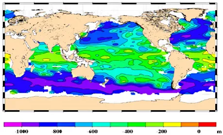
Fig. 5. Depth to which it is sufficient to integrate the DHA signals in order to explain 80% of the variance of the DHA calculated with a 1000 m depth reference level (the scale range from−1000 to 0).
5 Influence of the vertical structure of the ocean
To better understand the role of the vertical structure of the ocean on the correlation between SLA and DHA, DHA have been calculated relative to several depths from 100 m to 1000 m every 100 m. The depth to which it is sufficient to integrate the DHA signals in order to explain 80% of the variance of the DHA calculated with a 1000 m depth refer-ence level is first given on Fig. 5. The figure shows that the percentage is mainly a function of the latitude. At the equa-tor, a depth of 300 to 400 m is sufficient while a depth of at least 700 m is needed at high latitudes and in the Gulf Stream and the ACC.
The mean correlations between SLA and DHA have then been calculated by latitude bands (Fig. 6-left) as a function of depths used to calculate DHA. The latitudinal and hemi-spheric differences are clear. In the Northern Hemisphere, low latitudes reach the asymptote value of 0.85 at only 200 m of depth. At mid-latitudes, the correlation is of the order 0.74 at 200 m and increases slowly until it reaches 0.85 around 600 m. At high latitudes, the correlation evolves more reg-ularly from 0.68 at 200 m to 0.8 at 1000 m. For all North-ern Hemisphere latitudes, the correlation between SLA and DHA reach an asymptote value at depth, meaning that most part of the baroclinic signal is contained in the first 1000 m depth of the ocean. In the Southern Hemisphere, only the low latitudes reach an asymptote value. Mid and high lat-itudes SLA/DHA correlation start at a lower value than for the Northern Hemisphere but increase twice as rapidly with depth and do not reach a plateau. This means that the deep baroclinic signals not represented using a 1000 m depth ref-erence level would further improve the correlation between SLA and DHA.
Fig. 6. Correlation between SLA and DHA by latitude bands as a function of depth used to calculated DHA, for the Northern Hemi-sphere (top) and the Southern HemiHemi-sphere (bottom) and for to-tal SLA/DHA (left) and for SLA/DHA filtered from the seasonal means.
from SLA and DHA time series. SLA monthly means have been calculated on the studied period and the Arivo monthly climatological fields have been used for the DHA. Results have been compared to the ones obtained in the previous sec-tion and they show very similar patterns. For the intra sea-sonal signals, the evolutions of SLA/DHA correlation with depths (Fig. 6-right) show much smaller values than for the total signal and show very similar behaviors for the Northern and Southern Hemisphere. Intra seasonal SLA/DHA correla-tion rapidly reaches a plateau of 0.6 at low latitude. For mid and high latitudes, no plateau is reached and the increase of correlation with depth is of the order of 0.3 between 200 m and 1000 m depth.
To summarize, it implies that the high vertical coherence of the mesoscale variability is partly masked by the domi-nant signal due to heating/cooling of the surface ocean in the Northern Hemisphere. In the Southern Hemisphere, as the amplitude of the seasonal heating/cooling is half as large as in the Northern Hemisphere (Stammer, 2007), the signature of mesoscale variability and its coherency with depth is al-ready evident in the total SLA/DHA correlation (and even more obvious for intra-seasonal signals).
to 1.9 mm yr−1for the interannual time scales (Cazenave et al., 2008; Leuliette and Miller, 2009). The budget of global mean sea level is currently well documented. Second, in terms of regional analysis, SLA minus DHA signals have been less documented and can reveal deep ocean circulation patterns. A global seasonal mapping of these patterns has been performed by GLL06 and some of them were related to wind forcing mechanisms. Thanks to the Argo datasets, GLL06 seasonal cartography is revisited here and extended to interannual analysis.
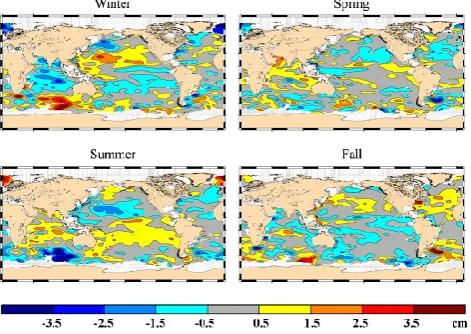
At seasonal time scales, the temporal and geographical distributions of the observations allow an almost global cov-erage. At 1000 m depth, SLA minus DHA signals differences show amplitudes of the order of 1 to 3 cm with minimum and maximum values in winter and summer respectively (Fig. 7). These patterns are similar to the ones described at 700 m depth by GLL06 but with lower amplitudes, due to the deeper reference level. Results obtained here with better data sets confirm and extend the ones from the previous study. Com-paring the two studies confirm, moreover, that the seasonal cycle of dynamic height is much more dependent on temper-ature than on salinity (Vinogradov et al., 2008; Ivchenko et al., 2008).
Fig. 7. Seasonal variation of the differences between SLA and DHA. Boxes with less than 10 observations are masked.
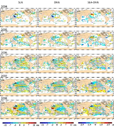
Even if the Argo datasets reached its initial target of 3000 operating floats worldwide only in November 2007, it is now possible to study interannual SLA minus DHA signals back to the year 2004. Variations of SLA, DHA, and SLA-DHA have been first calculated for each season of each year from 2004 to 2008, keeping only boxes with at least 5 observa-tions. Annual means are then calculated from the four sea-sonal means by keeping only the boxes validated for the four seasons. Each box is thus calculated using a minimum of 20 observations. Even if the coverage is far from been global in 2004, it increases rapidly with a good coverage of the Pacific Ocean from 2006. Large gaps remain in the Atlantic Ocean since large portion of Atlantic floats suffers from pressure offset errors and have not been used here.
At interannual time scales and on a 5 yr period, the spa-tial structure of SLA and DHA signals is dominated by the interannual to decadal variability and not the long term drift (Fig. 8). SLA and DHA signals are very consistent in all three oceans. For example, the tropical Pacific Ocean which is dominated by the El-Ni˜no/La-Ni˜na events shows very sim-ilar patterns in both data sets. The strong La-Ni˜na structure is particularly well reproduced in 2008 with enhanced sea level amplitudes in the Indian and Pacific oceans. Systematic dif-ferences between SLA and DHA are nevertheless visible at basin-scale. An interesting feature is that amplitudes of these differences are very similar to the ones observed for the sea-sonal signals and range from 1 to 3 cm. A shift from negative to positive values is for example observed for the whole In-dian Ocean (from−2 cm to 1 cm) between the year 2005 and the year 2006 reminding in basin-scale mass redistribution. The South Pacific Ocean also shows negative differences in 2005 and 2006 but positives ones in 2007 and again mainly negatives values in 2008. The opposite is observed in the North Pacific Ocean. For the Atlantic Ocean, the structures are very noisy and no clear tendency is visible.
Seasonal and interannual SLA minus DHA signals have been described here very qualitatively and future work is, in any case, needed to understand the observed differences and related them to different forcing mechanisms. They show, however, the new capability offered by the combined use of Argo and satellite altimetry observations to map these sig-nals.
7 Conclusions
The global Argo array of profiling floats is used together with satellite altimeter measurements of SLA in order to study the differences and complementarities between SLA and DHA calculated from the Argo temperature and salinity profiles. Results show very good correlation between the two data sets which is necessary to jointly use the two complemen-tary data sets in ocean forecasting models or data synthesis methodologies (Willis et al., 2003; Guinehut et al., 2004).
Compared to the previous study of GLL06, the newly available Argo data set bring about a series of improvements. The first one is a much better spatial coverage of all oceans and particularly of the Southern Ocean. The Argo array now allows sampling everywhere in all weather. This is particu-larly true during the harsh winter time conditions at high lat-itudes. The second improvement arises from the possibility to calculate a contemporaneous Argo mean dynamic height versus the use of climatological mean dynamic height, al-lowing improving the SLA/DHA consistency by 15%. The third improvement arises from the availability of deeper mea-surements and hence the use of a deeper reference level of 1000 m compared to 700 m, corresponding to an improve-ment of 12%. The fourth and the more important one in terms of SLA/DHA consistency increase (∼35%) concerns the use of measuredT andS profiles from Argo versus the use of climatologicalSprofiles. The Argo array also revolu-tionized the ocean salinity measurements and thus opens new insight on salinity variability studies.
The availability of observations along the Argo floats tra-jectories allows the description of the vertical structure of the ocean in term of baroclinic and barotropic contributions to sea level for the low frequency and mesoscale part of the circulation. Sea level variability is clearly dominated by baroclinic motion at seasonal to inter-annual periods, and for all latitudes. In the tropics, sea level variability is baro-clinic at all periods and at high latitudes, for intra seasonal and mesoscale signals, sea level variability is barotropic with also large influence of deep baroclinic signals. These results emphasize the need to separate the different time and space scales when altimeter and Argo data are jointly assimilated to estimate the 3-D temperature and salinity structure of the ocean.
Fig. 8. Annual variations of SLA, DHA, and SLA-DHA for the years 2004 to 2008. Boxes with less than 20 observations (5 observations for each season, see text) are masked.
qualitatively and show spatially coherent structures in the In-dian and Pacific Ocean. These signals are related to deep ocean circulation variations or basin-scale ocean mass vari-ations. Future work is needed to understand the observed differences and relate them to different forcing mechanisms. The comparison with Argo deep velocity observations and GRACE ocean mass variations should be, in particular, very instructive.
However, the improvements allowed by the Argo dataset in the comparison between the DHA and the SLA are not currently sufficient to study small-scale signals. Firstly, the Argo array does not allow meso-scale structure observations even if the spatial temporal resolution of the data is good. Secondly, altimetry maps that we used are not instantaneous fields, but the average of the available measures in a temporal
window of 7 days. More Argo data and a better temporal resolution of altimetry maps would allow pursuing the study through smaller-scales.
Acknowledgements. The Argo data were collected and made freely available by the international Argo project (a pilot program of the Global Ocean Observing System) and the na-tional programs that contribute to it (http://www.argo.ucsd.edu, http://argo.jcommops.org). The altimeter products were produced by SSALTO/DUACS and distributed by AVISO with support from CNES.
References
Antonov, J. I., Boyer, T. P., Mishonov, A. V., and Garcia, H. E.: Salinity. Vol. 2, World Ocean Atlas 2005, NOAA Atlas NESDIS, 65, 182 pp., 2006.
AVISO: Ssalto/Duacs user Handbook: (M)SLA and (M)ADT near-real time and delayed time products, SALP-MU-P-EA-21065-CLS, Edition 2.2, 2010.
Bell, M. J., Lefebvre, M., Le Traon, P. Y., Smith, N., and Wilmer-Becker, K.: The Global Ocean Data Assimilation Experiment, Oceanography, 22(3), 14–21, 2009.
Cazenave, A., Dominh, K., Guinehut, S., Berthier, E., Llovel, W., Ramilien, G., Ablain,M., and Larnicol, G.: Sea level budget over 2003–2008: A reevaluation from GRACE space gravimetry, satellite altimetry and Argo, Global Planet. Change, 65, 83–88, 2008.
Gaillard, F. and Charraudeau, R.: New climatology and statistics over the global Ocean, MERSEA-WP05-CNRS-STR-001-1A, 2008.
Guinehut, S., Le Traon, P.-Y., Larnicol, G., and Philipps, S.: Com-bining Argo and remote-sensing data to estimate the ocean three-dimensional temperature fields – a first approach based on simu-lated observations, J. Marine Syst., 46, 85–98, 2004.
Guinehut, S., Le Traon, P.-Y., and Larnicol, G.: What can we learn from Global Altimetry/Hydrography comparisons?, Geo-phys. Res. Lett., 33, L10604, doi:10.1029/2005GL025551, 2006. Ivchenko V. O., Danilov, S., Sidorenko, D.,Schr¨oter, J., Wenzel, M., and Aleynik, D. L.: Steric height variability in the Northern Atlantic on seasonal and interannual scales, J. Geophys. Res., 113, C11007, doi:10.1029/2008JC004836, 2008.
Leuliette, E. W., and Miller, L.: Closing the sea level rise bud-get with altimetry, Argo, and GRACE, Geophys. Res. Lett., 36, L04608, doi:10.1029/2008GL036010, 2009.
Locarnini, R. A., Mishonov, A. V., Antonov, J. I., Boyer, T. P., and Garcia, H. E. : Temperature. Vol. 1, World Ocean Atlas 2005, NOAA Atlas NESDIS, 61, 182 pp., 2006.
Penduff, T., Juza, M., Brodeau, L., Smith, G. C., Barnier, B., Mo-lines, J.-M., Treguier, A.-M., and Madec, G.: Impact of global ocean model resolution on sea-level variability with emphasis on interannual time scales, Ocean Sci., 6, 269–284, doi:10.5194/os-6-269-2010, 2010.
Roemmich, D., Belbeoch, M., Belchi, P. J. V., Freeland, H., Gould, W. J., Grant, F., Ignaszewski, M., Klein, B., Mork, K. A., Owens, W. B., Pouliquen, S., Ravichandran, M., Riser, S., Sterl, A., Suga, T., Suk, M.-S., Sutton, P., Thierry, V., Le Traon, P. Y., Wijffels, S., and Xu, J.: Argo: the challenge of continuing 10 years of progress, Oceanography, 22(3), 46–55, 2009.
Stammer D.: Steric and wind-induced changes in TOPEX/POSEIDON large-scale sea surface topography observations, J. Geophys. Res., 102(C9), 20987–21010, 2007. Vinogradov, S. V., Ponte, R. M, Heimbach, P., and Wunsch, C.:
The mean seasonal cycle in sea level estimated from a data-constrained general circulation model, J. Geophys. Res., 113, C03032, doi:10.1029/2007JC004496, 2008.
Vinogradova, N. T., Ponte, R. M., and Stammer, D.: Relation between sea level and bottom pressure and the vertical depen-dence of oceanic variability, Geophys. Res. Lett., 34, L03608, doi:10.1029/2006GL028588, 2007.
Willis, J. K., Roemmich, D., and Cornuelle, B.: Combining altimet-ric height with broadscale profile data to estimate stealtimet-ric height, heat storage, subsurface temperature, and sea-surface tempera-ture variability. Journal of Geophysical Research, 108(C7), 3292, doi:10.1029/2002JC001755, 2003.