https://doi.org/10.5194/se-9-385-2018
© Author(s) 2018. This work is distributed under the Creative Commons Attribution 4.0 License.
Monte Carlo simulation for uncertainty estimation on structural
data in implicit 3-D geological modeling, a guide for disturbance
distribution selection and parameterization
Evren Pakyuz-Charrier1, Mark Lindsay1, Vitaliy Ogarko2, Jeremie Giraud1, and Mark Jessell1
1Centre for Exploration Targeting, The University of Western Australia, 35 Stirling Hwy, Crawley WA 6009, Australia 2The International Centre for Radio Astronomy Research, The University of Western Australia,
35 Stirling Hwy, Crawley WA 6009, Australia
Correspondence:Evren Pakyuz-Charrier ([email protected]) Received: 10 October 2017 – Discussion started: 17 October 2017
Revised: 26 February 2018 – Accepted: 13 March 2018 – Published: 6 April 2018
Abstract. Three-dimensional (3-D) geological structural modeling aims to determine geological information in a 3-D space using structural data (foliations and interfaces) and topological rules as inputs. This is necessary in any project in which the properties of the subsurface matters; they ex-press our understanding of geometries in depth. For that rea-son, 3-D geological models have a wide range of practical applications including but not restricted to civil engineering, the oil and gas industry, the mining industry, and water man-agement. These models, however, are fraught with uncertain-ties originating from the inherent flaws of the modeling en-gines (working hypotheses, interpolator’s parameterization) and the inherent lack of knowledge in areas where there are no observations combined with input uncertainty (observa-tional, conceptual and technical errors). Because 3-D geolog-ical models are often used for impactful decision-making it is critical that all 3-D geological models provide accurate esti-mates of uncertainty. This paper’s focus is set on the effect of structural input data measurement uncertainty propagation in implicit 3-D geological modeling. This aim is achieved using Monte Carlo simulation for uncertainty estimation (MCUE), a stochastic method which samples from predefined distur-bance probability distributions that represent the uncertainty of the original input data set. MCUE is used to produce hun-dreds to thousands of altered unique data sets. The altered data sets are used as inputs to produce a range of plausi-ble 3-D models. The plausiplausi-ble models are then combined into a single probabilistic model as a means to propagate uncertainty from the input data to the final model. In this paper, several improved methods for MCUE are proposed.
The methods pertain to distribution selection for input un-certainty, sample analysis and statistical consistency of the sampled distribution. Pole vector sampling is proposed as a more rigorous alternative than dip vector sampling for planar features and the use of a Bayesian approach to disturbance distribution parameterization is suggested. The influence of incorrect disturbance distributions is discussed and proposi-tions are made and evaluated on synthetic and realistic cases to address the sighted issues. The distribution of the errors of the observed data (i.e., scedasticity) is shown to affect the quality of prior distributions for MCUE. Results demonstrate that the proposed workflows improve the reliability of uncer-tainty estimation and diminish the occurrence of artifacts.
1 Introduction
simpli-fications of the natural world (Bardossy and Fodor, 2001) linked to errors about their inputs (data and working hypothe-ses), processing (model building) and output formatting (dis-cretization, simplification). Reason dictates that these models should incorporate an estimate of their uncertainty as an aid to risk-aware decision-making.
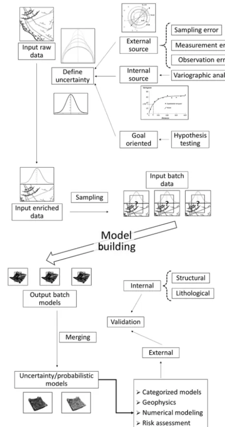
Monte Carlo simulation for uncertainty propagation (MCUE) has been a widely used uncertainty propagation method in implicit 3-D geological modeling during the last decade (Wellmann and Regenauer-Lieb, 2012; Lindsay et al., 2012; Jessell et al., 2014a; de la Varga and Wellmann, 2016). A similar approach was introduced to geoscience with the generalized likelihood uncertainty estimation (GLUE; Beven and Binley, 1992), which is a non-predictive (Camacho et al., 2015) implementation of Bayesian Monte Carlo (BMC). MCUE (Fig. 1) simulates input data uncertainty propaga-tion by producing many plausible models through pertur-bation of the initial input data; the output models are then merged and/or compared to estimate uncertainty. This can be achieved by replacing each original data input with a prob-ability distribution function (PDF) thought to best represent its uncertainty called a disturbance distribution. Essentially, a disturbance distribution quantifies the degree of confidence that one has in the input data used for the modeling such as the location of a stratigraphic horizon or the dip of a fault. In the context of MCUE, uncertainty in the input data mainly arises from a number of sources of uncertainty, including but not restricted to device basic measurement error, operator error, local variability, simplification radius, miscalibration, rounding errors, (re)projection issues and external perturba-tions. In the case of a standard geological compass used to acquire a foliation on an outcrop,
– device basic measurement error refers to error in lab and under perfect conditions (this information is typically provided by the manufacturer).
– operator error refers to human-related issues that affect the process of the measurement such as trembling or misinterpreting features (mistaking joints or crenulation for horizons for example).
– local variability refers to the difficulty of picking up the trend of the stratigraphy appropriately because of sig-nificant variability at the scale of the outcrop (usually due to cleavage or crenulation).
– simplification radius refers to the uncertainty that is in-troduced when several measurements made in the same area are combined into a single one.
– external perturbations refer to artificial or natural phe-nomena that have a detrimental effect on precision and accuracy such as holding high-magnetic-mass items close to the compass (smartphone, car, metallic struc-tures) when making a measurement or the magnetiza-tion of the outcrop itself.
Figure 1.Monte Carlo uncertainty propagation procedure work-flow.
been used to express the model uncertainty in MCUE, includ-ing information entropy (Shannon, 1948; Wellmann, 2013; Wellmann and Regenauer-Lieb, 2012), stratigraphic variabil-ity (Lindsay et al., 2012) and kriging error. The case for re-liable uncertainty estimation in 3-D geological modeling has been made repeatedly and this paper aims to further improve several points of MCUE methods at the preprocessing steps (Fig. 1). More specifically, we aim to improve (i) the selec-tion of the PDFs used to represent uncertainties related to the original data inputs and (ii) the parameterization of said PDFs. Section 2 reviews the fundamentals of MCUE meth-ods while Sect. 3 addresses PDF selection and parameteriza-tion. Lastly, Sect. 4 expands further into the details of distur-bance distribution sampling.
2 MCUE method
Recently developed MCUE-based techniques for uncertainty estimation in 3-D geological modeling require the user to de-fine the disturbance distribution for each input datum, based on some form of prior knowledge. That is necessary because MCUE is a one-step analysis as opposed to a sequential one: all inputs are perturbed once and simultaneously to generate one of the possible models that will be merged or compared with the others. MCUE is vulnerable to erroneous assump-tions about the disturbance distribution in terms of structure (what is the optimal type of disturbance distribution) and magnitude (the dispersion parameters) of the uncertainty of the input data. However, it is possible to post-process the re-sults of an MCUE simulation to compare them to other forms of prior knowledge and update accordingly (Wellmann et al., 2014a).
The MCUE approach is usually applied to geometric mod-eling engines (Wellmann and Regenauer-Lieb, 2012; Lind-say et al., 2013; Jessell et al., 2010, 2014a), although it can be applied to dynamic or kinematic modeling engines (Wang et al., 2016; Wellmann et al., 2016). This choice is motivated by critical differences between the three approaches, at both the conceptual and practical level (Aug, 2004). More specif-ically, explicit geometric engines require full expert knowl-edge while implicit ones are based on observed field data, variographic analysis and topological constraints (Jessell et al., 2014a). Geometric modeling engines interpolate features from sparse structural data and topological assumptions (Aug et al., 2005; Jessell et al., 2014a); they require prior knowl-edge of topology and are computationally affordable (La-jaunie et al., 1997; Calcagno et al., 2008). Dynamic model-ing engines require knowledge of initial geometry, physical properties and boundary conditions; the modeling process is computationally expensive. Kinematic modeling engines re-quire knowledge of initial geometry and kinematic history (Jessell, 1981); the modeling process is computationally in-expensive. The implicit geometric approach is preferred for MCUE because knowledge of initial conditions is nearly
im-possible to achieve, and perfect knowledge of current condi-tions defeats the purpose of estimating any uncertainty.
Implicit geometric modeling engines use mainly three types of inputs: interfaces (3-D points), foliations (3-D vec-tors) and topological relationships between geological units and faults (stratigraphic column and fault age relationships). Drill holes and other structural inputs such as fold axes and fold axial planes can also be used (Maxelon and Mancktelow, 2005). Each data input is assigned to a geological unit and the model is then built according to predefined topological rules. The implicit geometric 3-D modeling package GeoModeller distributed by Intrepid Geophysics was used as a test plat-form for this study. The use of this specific software is moti-vated by its open use of co-kriging (Appendix C), which is a robust (Matheron, 1970; Isaaks and Srivastava, 1989; Lajau-nie, 1990) geostatistical interpolator to generate the models (Calcagno et al., 2008; FitzGerald et al., 2009). In addition, GeoModeller allows uncertainty to be safely propagated pro-vided that the variogram is correct (Chilès et al., 2004; Aug, 2004) as the co-kriging interpolator then quantifies the its intrinsic uncertainty. Nevertheless, MCUE is not inherently limited by the choice of the interpolator and, therefore, may be used with any implicit modeling engine. In the next sec-tion, a series of improvements are proposed to address the disturbance distribution problem.
3 Distribution types and their parameters
Often, the disturbance distribution used to estimate input un-certainty is the same (same type and same parameterization) for all observations of the same nature (Wellmann et al., 2010; Wellmann and Regenauer-Lieb, 2012; Lindsay et al., 2012, 2013). Disturbance distribution parameters are defined arbitrarily (Lindsay et al., 2012; Wellmann and Regenauer-Lieb, 2012) in most cases. Additionally, uniform distribu-tions have been regularly used as disturbance distribution and expressed as a plus minus range over the location of inter-faces (Wellmann et al., 2010; Wellmann, 2013) or the dip and dip direction (Lindsay et al., 2012, 2013; Jessell et al., 2014a). Here, propositions are made about the type of dis-turbance distributions that should be used for MCUE, how to parameterize them and associated possible pitfalls.
3.1 Standard distributions for MCUE
indepen-dent trial in terms of its measurement error. Consequently, MCUE may sample from disturbance distributions indepen-dently from one another. Under these conditions, the cen-tral limit theorem (CLT) holds true for these data (Sivia and Skilling, 2006; Gnedenko and Kolmogorov, 1954) if the vari-ance of each source of uncertainty is always defined. Uncer-tainty would then be better represented by disturbance distri-butions that are consistent with the CLT, namely the normal distribution for locations (Cartesian scalar data) and the von Mises–Fisher (vMF) distribution for orientations (spherical vector data; Davis, 2003). However, MCUE does not a priori forbid the use of any kind of distribution. The normal distri-bution is the canonical CLT distridistri-bution (i.e., the distridistri-bution towards which the sum of random variables tends) defined as
N (x|ε, σ )=e −(x−ε)2
/2σ2 σ
√
2π , (1)
whereεandσ are the arithmetic mean and standard devia-tion, respectively. Note that the normal distribution is con-jugate to itself or to Student’s t distribution depending on which parameters are known a priori. That is, a normal prior distribution gives a normal or Student posterior distribution in the Bayesian framework given that the likelihood function is normal itself.
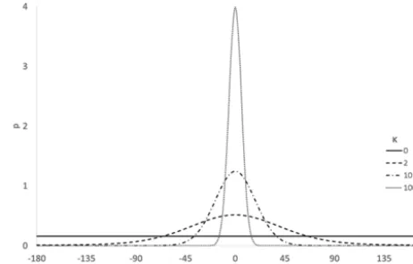
The vMF distribution (Fig. 2) is the CLT distribution for spherical data; it is the hyperspherical counterpart to the normal distribution (Fisher et al., 1987) and is used under the same general assumptions for unit vectors on the p -dimensional unit hypersphere S(p−1)1. The most important property of the vMF distribution is the axial symmetry of the data around the mean direction. The vMF distribution is also the maximum entropy distribution for spherical data and is conjugate to itself given that the likelihood function is vMF distributed (Mardia and El-Atoum, 1976). These properties make the vMF distribution suitable for uncertainty analysis of spherical data (Hornik and Grün, 2013). Sampling from the vMF distribution is described in Appendix A. The gen-eral probability density of the vMF distribution for Sp−1is expressed as follows
vMF(x|γ , κ)=Cp(κ) eκγ Tx
, κ >0 and||γ|| =1, (2) whereγTis the transposed mean direction vector andκis the concentration.|| ||denotes the Euclidean norm.κ is analo-gous to the inverse of σ for the normal distribution. High κ values denote distributions with low variance (Fig. 2), ul-timately leading to a p-dimensional hyperspherical Dirac distribution andκ=0 means complete randomness (equiva-lent to ap-dimensional hyperspherical uniform distribution). Bear in mind thatκ impacts the shape of the vMF distribu-tion exponentially (Fig. 2). Therefore, confidence intervals 1HereSp−1 denotes the surface of the p-dimensional
hyper-sphere.
Figure 2.Von Mises–Fisher probability distribution function on S1 (p=2) for various concentrationsκ.
are not linearly correlated toκ. For example, the 95% half aperture confidence interval forκ=1 is 150◦,κ=10 is 37◦ andκ=100 is 11◦.C
p(κ)is a normalization constant given
by
Cp(κ)=
κp/2−1
(2π )p/2Iv=p/2−1(κ)
, (3)
whereIv(κ)is the modified Bessel function of the first kind
at orderv, andpthe dimensionality ofS(p=3 forS2). 3.2 Disturbance distribution parameterization
compatible likelihood function to generate a predictive pos-terior disturbance distribution. The following demonstration applies to both the normal and the vMF distributions.
The uncertainty about an input structural datum (location or orientation) can be described by a distributionG
G=p (x|µtrue, ϑtrue) , (4)
whereµtrueandϑtrueare the true mean and dispersion of the population, respectively. Measured data at a single location are an-sized sampleX= {x1, . . ., xn}ofG. The disturbance
distribution that should be used for MCUE must take into account prior knowledge aboutϑtrue and the observed data X. This is achieved through a simple application of Bayes’ theorem:
p (µ|X, ϑ )=∝p (X|µ, ϑ ) p (µ, ϑ ) , (5) whereµandϑare the expression of prior knowledge about µtrueandϑtrue, respectively. The dispersionϑtrueis expected to be a deterministic function estimated via rigorous metro-logical studies, the methodology of which is beyond the scope of this paper. Thus, Eq. (5) simplifies to
p (µ|X)=∝p (X|µ) p (µ) . (6)
The prior distribution function p (µ)expresses prior belief about µ. In this case,p (µ)is defined as Jeffreys improper prior (Sivia and Skilling, 2006) for locations to express a complete lack of knowledge aboutp (µ):
ploc(µ)=const, (7)
and, for the same reason, as a uniform spherical distribution for orientations:
pori(µ)= 1
4π. (8)
The likelihood distributionp(X|µ)expresses the probability of observingXgivenµand is obtained under the assumption of independence by computing the joint density function for X:
p (X|µ)=
n
Y
i=1
p (xi|µ) . (9)
The posterior predictive distribution p xˆ|X
expresses the theoretical distribution of a new observation givenX regard-less ofµ; it is the target disturbance distribution to be sam-pled for MCUE and is given by
p xˆ|X= Z
p ( µ|X) p xˆ|X, µdµ, (10)
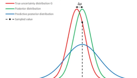
Figure 3.Effect of bias over predictive posterior and posterior dis-tributions.
wherexˆis the element to be sampled. To illustrate the ratio-nale for the usage of Eq. (10), one may consider the following example.
When a single measurement is made at a specific loca-tion, the sample size is 1(X = {x1})and the observed av-erage is equivalent to the measurement itself(µ≡x1). As-suming that the dispersion function is deterministic then ϑtrue is known. Obviously, the posterior distribution will be p (µ=x1|X=x1)=p (x|x1, ϑtrue). One might think that p (µ=x1|X=x1)is the target disturbance distribution that should be used for the perturbation step. However, doing so would lead to systematic underestimation of the effect of ϑtrue because p (µ|X) only quantifies the knowledge of µ in regard to x1. Indeed p (µ|X) tells about all the pos-sible Gvalues that x1 might be sampled from; it is a dis-tribution of the average and, ultimately, how farµ is from µtrue is (and will remain) unknown (Fig. 3). That is, sam-pling directly from p (µ|X) ignores the fact that 1µ= q
(µ−µtrue)2 is unknown. Such a procedure would intro-duce an undesired unknown bias to the perturbation step. To account for this,p (µ|X)is compounded to itself to ob-tain p (x|p (µ|X) , ϑtrue), which is equivalent to (10) and practically amounts to a double sampling ofp (µ|X). Con-sequently, regardless of the quality of the prior knowledge aboutϑtrue, sampling from the posterior predictive distribu-tion is better than sampling from the posterior distribudistribu-tion.
For a normal distribution, the posterior predictive distribu-tionpNis
pN xˆ|X∼N
x
µ0, σ2+ σ2
n
, (11)
pvMF xˆ|X∼vMF(x|vMF(µ0, κR) , κ) ≈vMF x
µ0, κR 1+R
, (12)
whereµ0andκand are the mean direction vector of the sam-ple and prior concentration (Appendix B) of the observed sample. Note that Eqs. 11 and 12 can be applied to data recorded as a mean value provided that the size of the sample is known.
In Eq. (12)µ0is given by
µ0=(sinφcosθ,sinφsinθ,cosφ) , (13) where
sinφ=Xn
i=1sinφi;sinθ= Xn
i=1sinθi; cosθ=Xn
i=1cosθi, (14)
where φ is the colatitude, θ is the longitude and R is the resultant length of the observed sample.
In Eq. (12)Ris given by
R= h
(sinφcosθ )2+(sinφsinθ )2+(cosφ)2 i12
. (15)
From Eqs. (11) and (12) it appears that sampling from prior distributions directly will lead to systematic underestimation of dispersion because σ2≥σ2
n and κ≤ κR
1+R. In turn, this
bias will narrow the range of models explored by MCUE and will make the final results look less uncertain than they should be. This is highly important because disturbance dis-tribution sampling in MCUE is a one-step process and incor-rect disturbance distributions are not to be updated or refined at any point. Therefore, accurate parameterization of a dis-turbance distribution at the beginning of the process is cru-cial to ensure accurate sampling. Bayesian schemes exist to validate models based on some external observations or as-sumptions (Fig. 1) that are used to build likelihood functions (de la Varga and Wellmann, 2016). However, these schemes are known to not yield good results when incorrect informa-tive priors are used (Freni and Mannina, 2010; Morita et al., 2010). Incorrect informative priors have low dispersion (high precision, “self-confident”) and high bias (low accuracy, “off target”). This results in an inability of standard Bayesian schemes to update these priors regardless of the strength of the evidence. For example, a posterior distribution extracted from a single foliation measured on an outcrop cannot be used as a disturbance distribution. Indeed, it is too narrow and may be heavily biased (Fig. 3). To avoid this detrimen-tal effect, one should instead sample from the posterior pre-dictive distributions (Eqs. 11, 12) for more accurate results about uncertainty.
3.3 Measurement scedasticity
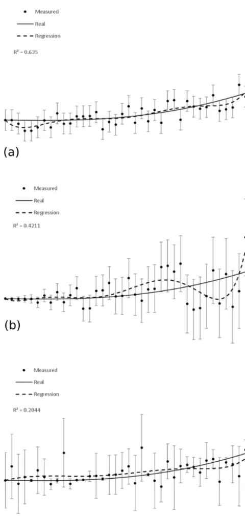
Scedasticity is defined as the distribution of the error about measured or estimated elements of a random variable of in-terest (Levenbach, 1973). It expresses the relationship be-tween the measured values and their uncertainty. In the case in which uncertainty is constant across the variable space the variable is homoscedastic (Fig. 4a); such behavior is commonly assumed in gravity surveys (Middlemiss et al., 2016). When uncertainty is not constant throughout the vari-able space, the varivari-able is called heteroscedastic (Fig. 4b, c). Note that heteroscedastic cases include both structured (Fig. 4b) and unstructured (Fig. 4c) relationships between the measured values and their respective errors. Structured heteroscedastic variables show a clear relationship (e.g., cor-relation, cyclicality) between the variable and its uncertainty while unstructured ones do not. Structured heteroscedastic behavior is observed electrical resistivity tomography (Per-rone et al., 2014), magnetotellurics (Thiel et al., 2016; Rawat et al., 2014), airborne gravity and magnetics (Kamm et al., 2015), and controlled-source electromagnetic (Myer et al., 2011) surveys. It is usually possible to transform a struc-tured heteroscedastic variable to a space where it becomes homoscedastic (commonly the log space), perform analysis and transform back to the original space. Unstructured het-eroscedastic behavior is common in seismic surveys and im-pacts inversions (Kragh and Christie, 2002; Quirein et al., 2000; Eiken et al., 2005). The heteroscedastic case essen-tially allows for any level of correlation between the mea-sured values and their uncertainty or error to be possible (Fig. 5).
The failure to account for scedasticity often implies the as-sumption of homoscedasticity as this asas-sumption allows for a wider range of statistical methods to be applied. With het-eroscedastic data, the results of methods that depend on the assumption of homoscedasticity, such as least-squares meth-ods (Fig. 4), give results of much decreased quality (Eubank and Thomas, 1993) and this may lead to the validation of in-correct hypotheses. Scedasticity analysis from raw data with-out prior knowledge is challenging (Zheng et al., 2012) and this topic of research is still being investigated (Dosne et al., 2016). If there is no option for an appropriate transform, it is advisable to perform an empirical analysis of scedasticity beforehand. This is usually achieved through experimental assessment of uncertainty under various conditions (metro-logical study) of measurement and over the entire range of measured values (Allmendinger et al., 2017; Cawood et al., 2017; Novakova and Pavlis, 2017). The results of such anal-ysis can then be used to define the prior dispersion (ϑ in 5) more accurately as a function of the measurement instead of a constant.
Figure 4. Synthetic examples of different levels of scedastic-ity of measurements of the same variable. (a) Homoscedastic case,(b)structured heteroscedastic case and(c)unstructured het-eroscedastic case. Note how the least-square polynomial residual score (R2) is heavily impacted by scedasticity.
better defined when scedasticity is accounted for. It is worth mentioning that both the normal distribution and the von Mises–Fisher distribution have a complete range of analyti-cal or approximated solutions for both posterior and posterior predictive distributions (Rodrigues et al., 2000; Bagchi and
Figure 5.Distribution of errors for the cases described in Fig. 3. Homoscedastic case shows constant uncertainty and no relationship of uncertainty to the data. The structured heteroscedastic case has a linear relationship of uncertainty to the data. The unstructured het-eroscedastic case demonstrates no obvious relationship of uncer-tainty to the data and is not constant.
Guttman, 1988; Bagchi, 1987). In the next section, distur-bance distribution sampling for spherical data (orientations) is discussed.
4 Sampling of orientation data for planar features In the geoscience, the orientation of planar features such as faults and bedding is described by foliations. These folia-tions can be recorded in the form of dip vectors using the dip and dip-direction system. This system is equivalent to a reversed right-hand rule spherical coordinates system. The following covers sampling strategies for such spherical data and demonstrates their impact on MCUE results.
4.1 Artificial heteroscedasticity
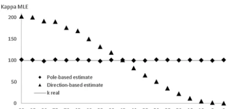
Figure 6.Distortion of the maximum likelihood estimation (MLE) of concentration or spherical variance of 100 spherical unit vector samples of a size of 1000 individuals drawn from a von Mises– Fisher distribution withκ=100. A pole-based estimate is always consistent with the data while dip-based ones either over- or under-estimate it.
plane, dip vectors distribute themselves directly below and about the equator ofS2, following a girdle-like distribution (Fig. 7a, b). Consequently, the resultant length is null and the spherical varianceSs2(Eq. 16) equals unity as the barycenter of all dip vectors is located at the center ofS2.
Ss2=1−R
n (16)
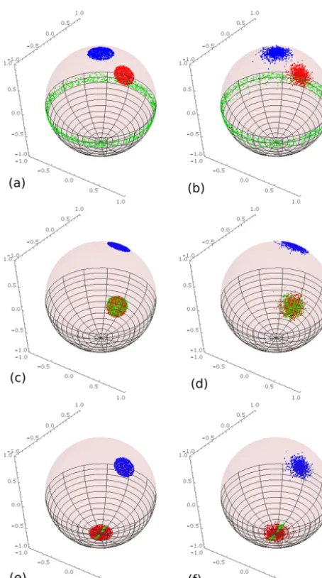
Naive interpretation of S2s may lead one to misinterpret un-certainty to be infinite Ss2=1and the plane’s orientation to be uniformly random where it might be very well constrained in reality. That is so because Ss2 is a scalar quantity used to represent dispersion for samples of spherical unit vectors. Therefore, it is expected thatSs2is ambiguous in some cases. The opposite effect occurs for (sub)vertical planes whereS2s will appear to be lower than expected. In Fig. 7, the effect of dip vector sampling and pole vector sampling is demon-strated for theoretical cases. Here, the blue clusters are the direct result of pole vector sampling and always describe the plane’s behavior accurately in terms of pole vectors. They have constant point density and are isotropic; parameteriza-tion is easy and reliable for distribuparameteriza-tions such as von Mises– Fisher (Fig. 7b, d, f) or bounded uniform (Fig. 7a, c, e). Green clusters are the result of pole vector sampling (blue) converted back to dip vector and they describe the plane’s behavior accurately in terms of dip vectors. These clusters have varying shapes and may not be modeled satisfactorily by any existing spherical distribution for all possible cases. Red clusters are the direct result of dip vector sampling and fail to describe the behavior of the plane accurately. There-fore, accurate sampling based on dip vectors (green) is nearly impossible to achieve without increasing the number of pa-rameters of the distributions to take into account the afore-mentioned effects (i.e., adding a set of functions to compen-sate for scedasticity errors as well as boundary effects). For example, in a scenario in which dip vectors are used directly
to estimate a sample’s spherical variance or sample over a disturbance distribution, one may attempt to define separate values for dispersion of dip and dip direction (Lindsay et al., 2012) in order to compensate for scedastic incoherence. A horizontal plane’s uncertainty is then obtained by setting cir-cular variance as null over the dip direction and as any real positive value over the dip. In addition, some form of bound-ary control or polarity correction of the dip is necessbound-ary to remove incorrect occurrences. Conversely, poles to planes carry information about polarity implicitly (e.g., the Carte-sian pole of a horizontal plane is [0, 0, 1] while its reversed counterpart is [0, 0,−1]). Note that this method still does not solve the scedasticity issue entirely, especially for high uncertainty values about the dip and vertical dips. Similarly, if dip vectors are used directly, near-vertical planes display uniform random behavior of dip direction (Fig. 7e, f) instead of the expected “bow tie” pattern. This pattern is impossible to model accurately using CLT spherical distributions as they are unimodal and symmetric.
The use of distributions in MCUE makes it very sensi-tive to scedasticity over inputs. The uncertainty of a dip vec-tor which is quantified by any dispersion parameter similar toSs2 will show non-systematic heteroscedasticity because of variance distortion. A plane dipping at any angle would show increased heteroscedasticity of its uncertainty as the dispersion parameter used to parameterize the underlying distribution increases. Note that uncertain planes show in-creased heteroscedasticity as their dip diverges from a 45◦ dip (Fig. 7c, d). Boundary effects also play a role for hor-izontal and vertical limit cases (Figs. 6, 7) as standard dip angles are constrained to 0−π
Figure 7.Effect of sampling over dip vectors or pole vectors on bounded uniform spherical distribution at a range=10◦(a, c, e)and von Mises–Fisher distribution atκ=100.0(b, d, f)for uncertain horizontal planes(a, b), 45◦dip planes(c, d)and vertical planes(e, f). Correct (pole perturbed) dip vectors are green, incorrect (dip perturbed) dip vectors are red and blue vectors are the poles. See Sect. 4.1 for details.
4.2 Impact of pole vector sampling versus dip vector sampling
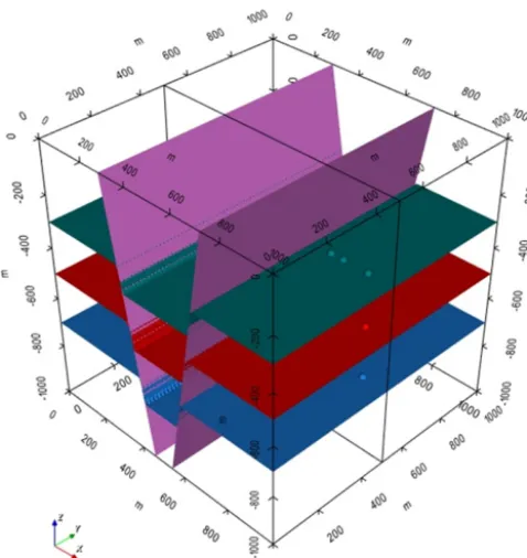
The impact of pole versus dip vector sampling on the results of MCUE is evaluated on a simple synthetic model and on a realistic synthetic model. The simple model is a standard symmetric graben with four horizontal units; it has been cho-sen for its simplicity and is commonly used as a test case (Wellmann et al., 2014b; de la Varga and Wellmann, 2016; Chilès et al., 2004) in MCUE for proof of concepts. The real-istic model is a modification of a real demonstration case that is part of the GeoModeller package based on a location near
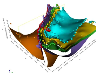
Mansfield, Victoria, Australia. It features a Carboniferous sedimentary basin oriented NW–SE that is in a faulted con-tact (Mansfield Fault) on its SW edge to a Silurian–Devonian set of older, folded basins. Outcropping units are almost all of the siliceous detritic type ranging from mildly deformed sandstones to siltstones and shales; the basement is made of Ordovician–Cambrian serpentinized sandstone. The orig-inal data for the Mansfield model were not altered in any way, instead data based on the Mansfield geological map (Cayley et al., 2006) geophysical map (Haydon et al., 2006) and airborne geophysical survey (Wynne and Bacchin, 2009; Richardson, 2003) were added to refine it.
The graben model is built using orientations and inter-faces only, with three interinter-faces and three foliations per unit and one interface and one foliation per fault (Figs. 8, 9c). The Mansfield model is built with 281 interface points and 176 foliations over six units and three faults (Figs. 10, 11c). For both models, perturbation is performed as described in Sect. 3. For the graben model, units’ interfaces are isotrop-ically perturbed over a normal distribution with the mean centered on the original data point and a standard deviation of 25 m. The orientations of the faults are perturbed over a von Mises–Fisher distribution with the original data as the mean vector and concentration of 100 (p95∼ ±10◦) fol-lowing the recommended pole vector procedure described in Sect. 4.1 (Figs. 9a, 11a) or the dip vector one (Figs. 9b, 11b). For the Mansfield model, all interfaces and orientations (both for units and faults) are perturbed using the parameterization given for the graben model. The perturbation parameters for orientations were chosen to be compatible with metrological data. That is, values for the dispersion of the spherical distur-bance distributions used for the foliations were estimated on the basis of the variability in plane measurements observed by other authors (Nelson et al., 1987; Stigsson, 2016; All-mendiger et al., 2017; Cawood et al., 2017; Novakova and Pavlis, 2017) in a variety of settings and for different types of devices. Perturbation parameters for interfaces were de-signed to meet observed GPS uncertainty (Jennings et al., 2010) and observed experimental interface variability in pre-vious authors’ works (Courrioux et al., 2015; Lark et al., 2014, 2013). More specifically it was assumed that the ob-served end variability in the interfaces’ locations in their models can be transposed to the presented cases. This is of course an approximation in the absence of specific metrolog-ical studies.
Figure 8.Structural data for the graben model and modeled surfaces for units and faults. Spheres represent interfaces and cones represent pole vectors.
11c) to be easily distinguishable. In cases in which the ori-entation data are more vulnerable to improper sampling error (away from 45◦dips) important structures such as the near-vertical faults in the graben model (Fig. 9) or the circled areas in Fig. 11 may completely disappear. It also appears that ar-eas where low uncertainty would be expected (orange unit in Fig. 11) are the loci of excess uncertainty. These observa-tions support the assertion that pole vector sampling should be favored to improve uncertainty propagation in MCUE.
5 Discussion
Generally, CLT distributions are valid choices as prior uncer-tainty distributions (and disturbance distributions) because they describe the behavior of uncertainty well. However, there may be scenarios in which alternatives can offer a bet-ter solution. More specifically, the uniform or the Laplace distribution may better describe location uncertainty than the normal distribution. The uniform distribution indicates a lack of constraints as to the prior uncertainty distribution; it is a valid choice when there is little knowledge about data dis-persion. The Laplace distribution is suitable if the measured data abide by the first law of errors instead of the second (Wilson, 1923). For example, to model the uncertainty on the thickness of a geological unit along a drill core, one might observe that the uncertainty of the location of the top and bottom interfaces of the unit is best represented by an
expo-nential distribution. In this instance, the Laplace distribution would be a suitable option to model the thickness’ uncer-tainty. Under similar circumstances, a spherical exponential distribution could be swapped with the vMF distribution. The Kent2distribution is also a good candidate to describe tation uncertainty when the pole vectors of measured orien-tations appear to be anisotropically distributed onS2(Kent and Hamelryck, 2005).
In this paper, it is explicitly assumed that the dispersion of prior uncertainty distributions is a deterministic function. Note that this does not necessarily make this function a con-stant and it might depend on the observed data. The disper-sion function of field measurements (using a compass) of structural data would be expected to be nearly constant. Con-versely, the dispersion function of interpreted measurements (using geophysics) would be expected to be dependent on the sensitivity of the intermediary method. Additionally, disper-sion functions may be probabilistic as well as deterministic (Bucher, 2012). Determinism is a strong assumption when no metrological study was conducted beforehand to assess its plausibility. Such metrological studies involve experimental testing of devices and procedures in order to estimate pre-cision, accuracy, bias, scedasticity or drift about measured data. These estimates can then be compiled into a dispersion function that can be used as an input parameter for other pur-poses, including prior uncertainty distributions for MCUE. Probabilistic dispersion functions apply non-negligible un-certainty to the dispersion function for prior unun-certainty dis-tributions. Uncertainty about dispersion makes the proposed workflow for disturbance distribution parameterization inad-equate. Indeed, Eq. (5) may not be simplified into Eq. (6) anymore and the following statements (Eqs. 7 to 14) would then ignore the probabilistic nature of the dispersion func-tion. Both the normal and the vMF distributions have ana-lytical solutions or good approximations for such cases; the authors recommend the readers refer to relevant works (Gel-man et al., 2014; Bagchi and Gutt(Gel-man, 1988) if required. Note that there is significant metrological work about bore-hole data (Nelson et al., 1987; Stigsson, 2016) as opposed to usual structural data such as foliations, fold planes, fold axes or interfaces.
Although the authors make the case for scedasticity anal-ysis in MCUE, it is left open in this paper. Scedasticity is essentially an untouched subject in geological 3-D modeling and it was pointed out to make the geological 3-D modeling community aware of this fact and its potentially nefarious in-fluence on MCUE outputs. However, standard metrological studies can determine scedasticity and include it in a disper-sion function to be a parameter of the prior uncertainty dis-tributions (Bewoor and Kulkarni, 2009; Bucher, 2012).
2The Kent distribution is the spherical analogue to a bivariate
Figure 9.Effect of pole(a)versus dip(b)perturbation for a graben model(c); orientations are perturbed over a vMF distribution with
κ=100.
Figure 10.Structural data for the Mansfield model and modeled surfaces for units and faults. Spheres are interfaces and cones are orientations.
The evidence brought at the theoretical and practical lev-els allows us to strongly advocate for the use of pole vec-tors over dip vecvec-tors. In fact, dip vector sampling shows poor performance away from 45◦ dip planes, induces artificial heteroscedasticity and requires specific polarity indicators. This especially applies to MCUE methods in which Bayesian post-analysis is performed for the probabilistic model that re-sults from basic propagation of uncertainty (de la Varga and
Figure 11.Effect of pole(a)versus dip(b)perturbation on a cross section of the Mansfield model(c); orientations are perturbed over a von Mises–Fisher distribution withκ=100.
features (lineations, fold axes, other planar features intersec-tions) for which the concept of a pole does not apply.
Good prior knowledge about input uncertainty is critical to the propagation of uncertainty in general. This, in turn, makes metrological work mandatory to any form of model-ing that relies on actual measured data. Note that it is ac-ceptable to use preexisting metrological studies to define the priors (Allmendinger et al., 2017; Cawood et al., 2017; No-vakova and Pavlis, 2017) provided that the measurement de-vice and procedure used are similar to those of the studies. To gather multiple observations per site is strongly recom-mended as this practice sharply increases the quality of the disturbance distributions. From a practical point of view this would require field operators to perform several measure-ments on the same outcrop. If that is not possible one may group measurements of clustered outcrops together provided that the scale of the modeled area compared to that of the cluster allows it. The authors recommend not grouping clus-ters that are spread out more than 3 orders of magnitude be-low the model size (e.g., for a 10 km×10 km model, clusters of radius higher than 5 m shall not be grouped). Note that more refined structural data upscaling methods have been recently proposed to address this specific issue (Carmichael and Ailleres, 2016). However, there is another major source of uncertainty that stems from the necessarily imperfect mod-eling engine itself. Implicit geometric modmod-eling engines (in this case, GeoModeller) use interpolation to draw the contact surfaces of geological units. Therefore, the parameterization of the interpolator may impact results. The co-kriging inter-polator (Appendix C) used in this paper relies on (uncertain) variographic analysis (Appendix C, Eq. C2) and is natively able to express its own uncertainty (Appendix C, Eq. 29). Therefore, these sources of uncertainty are expected to be
propagated along the input uncertainty as a hyperparameter in Eq. (5).
6 Conclusions
Propagation of uncertainty is the process through which dif-ferent kinds and sources of uncertainties about the same phe-nomenon are combined into a single final estimate. MCUE methods seek to achieve propagation of uncertainty using Monte Carlo-based systems in which input uncertainty is simulated through the sampling of probability distributions called a disturbance distribution. Disturbance distributions are the distributions that normally best represent the uncer-tainty about the input data in the context of unceruncer-tainty prop-agation in geological 3-D modeling.
to be the best alternative because it is guaranteed not to dis-tort the disturbance distribution shape or generate artifacts in the output uncertainty models the way dip vector sampling does.
The proposed framework and methods are compatible with previous MCUE work on 3-D geological modeling and can be easily added to existing implementations to improve their accuracy. As MCUE is applicable to all fields in which 3-D geological models are needed, so is the proposed framework. The primary domains of application are the mining and oil and gas industries at the exploration, development and pro-duction steps. In addition, numerous secondary domains of potential application are available to this work, such as civil engineering and fundamental research.
Appendix A: Von Mises–Fisher pseudo-random number generation
Von Mises–Fisher sampling on the usual sphere is not new (Wood, 1994) and this appendix serves as a reminder for the reader. To generate a von Mises–Fisher distributed pseudo-random spherical 3-D unit vector Xsphe onS2 for a given mean directionµand concentrationκ, define
Xsphe=[φ, θ, r]. (A1)
Forµ=[0, (.) ,1] the pseudo-random vector is given by
Xsphe=[arcosW, V ,1]. (A2)
V is given by
V ∼U (0,2π ) . (A3)
U (a, b)is the usual continuous uniform distribution. W is given by
W =1+1 κ
lnξ+ln
1−ξ−1
ξ e
−2κ, (A4)
where
ξ ∼U (0,1) . (A5)
Note that in Eq. A4,W is undefined forξ=0 and it should be set toW = −1 in this case.Xspheshould then be rotated to be consistent with the chosenµ.
Appendix B: Parameter estimates for von Mises–Fisher The maximum likelihood estimationµˆ ofµfor a given sam-ple ofnunit vectors onS2is the mean direction vector
ˆ
µ= R
kRk. (B1)
A simple approximation of the concentration parameterκˆ is estimated by (Banerjee et al., 2005)
ˆ κ=
Rp−R2
1−R2
, (B2)
where
R=R
n. (B3)
More refined techniques are available to compute this last es-timation (Sra, 2011) though they do not produce significantly better results for low-dimensionality cases (p < 5)with high values ofκ. Thus, it is recommended to use the above.
Appendix C: Co-kriging algorithm in GeoModeller The co-kriging algorithm used in GeoModeller interpolates a 3-D vector field and converts it into a potential (scalar) field (Calcagno et al., 2008; Guillen et al., 2008) that is then contoured to draw interface surfaces. The space between sur-faces is defined as belonging to a specific unit based on topo-logical rules. The topotopo-logical rules are set by (i) the strati-graphic column for units versus unit topological rules, (ii) the fault network matrix for faults versus fault topological rules and (iii) the fault affectation matrix for faults versus unit topological rules.
The potential field co-kriging interpolator is
T∗(p)−T∗(p0)=
M
X
α=1
µα T (pα)−T pα0
+
N
X
β=1 νβ
∂T ∂uβ
pβ, (C1)
whereT∗(p)−T∗(p0)is the potential difference at the point p given an arbitrary constant origin pointp0. The weights µα andνβ are the unknowns.Mis the number of interfaces
andNis 3×the number of foliations. For practical purposes, the modeled random functionT is considered to be affected by a polynomial drift that is deduced from the foliation data (Chilès and Delfiner, 2009). The theoretical semi-variogram is obtained through variographic analysis; it is then used to solve Eq. (C1) and is usually of the cubic (Eq. C2) type (Calcagno et al., 2008).
γ (d)=C 7
d a 2 −35 4 d a 3 +7 2 d a 5 −3 4 d a 7! , (C2)
whered and a are the lag distance and the range, respec-tively. The theoretical semi-variogram is fit to an empirical semi-variogram (Matheron, 1970). In practical cases, the em-pirical to theoretical semi-variogram fit is never perfect and is mostly parametric. The probability that the potential value estimated at a pointx is comprised betweent andt0 (Aug, 2004; Chilès et al., 2004) is given by
P t≤T∗(p)−T∗(p0) < t0=N
t0−t
σCK(x)
, (C3)
Competing interests. The authors declare that they have no conflict of interest.
Acknowledgements. The authors would like to thank the Geologi-cal Survey of Western Australia, the Western Australian Fellowship Program and the Australian Research Council for their financial support. In addition, the authors make special distinction to Intrepid Geophysics for their outstanding technical support. In addition, the authors express their gratitude to Ylona van Dinther, Guil-laume Caumon and Eric de Kemp, for their insightful comments and dedication to help us improve this paper.
Edited by: Ylona van Dinther
Reviewed by: Eric de Kemp and Guillaume Caumon
References
Aldiss, D. T., Black, M. G., Entwisle, D. C., Page, D. P., and Terrington, R. L.: Benefits of a 3-D geological model for major tunnelling works: an example from Farringdon, east-central London, UK, Q. J. Eng. Geol. Hydroge., 45, 405–414, https://doi.org/10.1144/qjegh2011-066, 2012.
Allmendinger, R. W., Siron, C. R., and Scott, C. P.: Structural data collection with mobile devices: Accuracy, redundancy, and best practices, J. Struct. Geol., 102, 98–112, 2017.
Aug, C.: Modelisation geologique 3-D et caracterisation des incer-titudes par la methode du champ de potentiel, PhD, Ecole des Mines de Paris, Paris, 220 pp., 2004.
Aug, C., Chilès, J.-P., Courrioux, G., and Lajaunie, C.: 3-D geolog-ical modelling and uncertainty: The potential-field method, in: Geostatistics Banff 2004, Springer, 145–154, 2005.
Bagchi, P.: Bayesian analysis of directional data, University of Toronto, Ottawa, Ont: National Library of Canada, 1987. Bagchi, P. and Guttman, I.: Theoretical considerations of the
multi-variate von Mises-Fisher distribution, J. Appl. Stat., 15, 149–169, 1988.
Banerjee, A., Dhillon, I. S., Ghosh, J., and Sra, S.: Clustering on the Unit Hypersphere using von Mises-Fisher Distributions, J. Mach. Learn. Res., 6, 1345–1382, 2005.
Bardossy, G. and Fodor, J.: Traditional and NewWays to Handle Uncertainty in Geology, Nat. Ressour. Res., 10, 179–187, 2001. Beven, K. and Binley, A.: The future of distributed models: model
calibration and uncertainty prediction, Hydrol. Process., 6, 279– 298, 1992.
Bewoor, A. K. and Kulkarni, V. A.: Metrology and measurement, McGraw-Hill Education, New Delhi, 2009.
Bucher, J. L.: The metrology handbook, edited by: Bucher, J. L., ASQ Quality Press, United States of America, 2012.
Calcagno, P., Chilès, J. P., Courrioux, G., and Guillen, A.: Geological modelling from field data and geologi-cal knowledge, Phys. Earth Planet. Int., 171, 147–157, https://doi.org/10.1016/j.pepi.2008.06.013, 2008.
Camacho, R. A., Martin, J. L., McAnally, W., Díaz-Ramirez, J., Ro-driguez, H., Sucsy, P., and Zhang, S.: A comparison of Bayesian methods for uncertainty analysis in hydraulic and hydrodynamic modeling, J. Am. Water Ressour. Assoc., 51, 1372–1393, 2015.
Cammack, R.: Developing an engineering geological model in the fractured and brecciated rocks of a copper porphyry de-posit, Geol. Soc. Lond. Eng. Geol. Spec. Publ., 27, 93–100, https://doi.org/10.1144/egsp27.8, 2016.
Carmichael, T. and Ailleres, L.: Method and analysis for the upscal-ing of structural data, J. Struct. Geol., 83, 121–133, 2016. Cawood, A. J., Bond, C. E., Howell, J. A., Butler, R. W., and
To-take, Y.: LiDAR, UAV or compass-clinometer? Accuracy, cov-erage and the effects on structural models, J. Struct. Geol., 98, 67–82, 2017.
Cayley, R. A., Osborne, C. R., and Vanderberg, A. H. M.: Mansfield 1:50 000 geological map, Geological Survey of Victoria, Geo-Science Victoria, Department of Primary Industries, Melbourne, 2006.
Chilès, J. P. and Delfiner, P.: Geostatistics: modeling spatial uncer-tainty, John Wiley & Sons, New Jersey, 2009.
Chilès, J. P., Aug, C., Guillen, A., and Lees, T.: Modelling the Ge-ometry of Geological Units and its Uncertainty in 3-D From Structural Data: The Potential-Field Method, Orebody Mod-elling and Strategic Mine Planning, Perth, 22 November 2004, 2004.
Courrioux, G., Allanic, C., Bourgine, B., Guillen, A., Baudin, T., Lacquement, F., Gabalda, S., Cagnard, F., Le Bayon, B., and Besse, J.: Comparisons from multiple realizations of a geological model, Implication for uncertainty factors identification, IAMG 2015: The 17th annual conference of the International Associa-tion for Mathematical Geosciences, 2015.
Davis, J. C.: Statistics and Data Analysis in Geology, 3rd Edn., Wi-ley, New Jersey, 656 pp., 2003.
de la Varga, M. and Wellmann, J. F.: Structural geologic modeling as an inference problem: A Bayesian perspective, Interpretation, 4, SM1–SM16, 2016.
Delgado Marchal, J., Garrido Manrique, J., Lenti, L., López Casado, C., Martino, S., and Sierra, F. J.: Unconventional pseudostatic stability analysis of the Diezma landslide (Granada, Spain) based on a high-resolution engineering-geological model, Eng. Geol., 184, 81–95, https://doi.org/10.1016/j.enggeo.2014.11.002, 2015. Dominy, S. C. N., Mark, A., and Annels, A. E.: Errors and Un-certainty in Mineral Resource and Ore Reserve Estimation: The Importance of Getting it Right, Explor. Min. Geol., 11, 77–98, 2002.
Dosne, A.-G., Bergstrand, M., and Karlsson, M. O.: A strategy for residual error modeling incorporating scedasticity of variance and distribution shape, J. Pharmacokinet. Phar., 43, 137–151, 2016.
Eiken, O., Haugen, G. U., Schonewille, M., and Duijndam, A.: D. A Proven Method for Acquiring Highly Repeatable Towed Streamer Seismic Data, in: Insights and Methods for 4D Reser-voir Monitoring and Characterization, Society of Exploration Geophysicists and European Association of Geoscientists and Engineers, 209–216, 2005.
Ennis-King, J. and Paterson, L.: Engineering Aspects of Geological Sequestration of Carbon Dioxide, Asia Pacific Oil and Gas Con-ference and Exhibition Melbourne, Australia, 8 October 2002, 2002.
Eubank, R. and Thomas, W.: Detecting heteroscedasticity in non-parametric regression, J. Roy. Stat. Soc. B, 55, 145–155, 1993. Fisher, N. I., Lewis, T., and Embleton, B. J.: Statistical analysis of
FitzGerald, D., Chilès, J. P., and Guillen, A.: Delineate Three-Dimensional Iron Ore Geology and Resource Models Using the Potential Field Method, Iron Ore Conference, Perth, 27 July 2009, 2009.
Freni, G. and Mannina, G.: Bayesian approach for uncertainty quan-tification in water quality modelling: The influence of prior dis-tribution, J. Hydrol., 392, 31–39, 2010.
Gelman, A., Carlin, J. B., Stern, H. S., and Rubin, D. B.: Bayesian data analysis, Chapman & Hall/CRC Boca Raton, FL, USA, 2014.
Gnedenko, B. and Kolmogorov, A.: Limit distributions for sums of independent, Am. J. Math., 105, 28–35, 1954.
Guillen, A., Calcagno, P., Courrioux, G., Joly, A., and Ledru, P.: Geological modelling from field data and geologi-cal knowledge, Phys. Earth Planet. Int., 171, 158–169, https://doi.org/10.1016/j.pepi.2008.06.014, 2008.
Haydon, S. J., Skladzien, P. B., and Cayley, R. A.: Parts of Mans-field Alexandra and Euroa 1:100 000 maps: Geological interpre-tation of geophysical features map, Geological Survey of Victo-ria, Geoscience VictoVicto-ria, Deparment of Primary Industries, Mel-bourne, 2006.
Hornik, K. and Grün, B.: On conjugate families and Jeffreys priors for von Mises–Fisher distributions, J. Stat. Plan. Infer., 143, 992– 999, 2013.
Intrepid Geophysics: “GeoModeller API” Intrepid Geophysics|Home of GeoModeller, Intrepid, Jetstream and Sea-g|Gravity, Magnetics, Radiometrics, FTG, available at: www. intrepid-geophysics.com/ig/index.php?page=geomodeller-api, last access: 19 February 2018.
Isaaks, E. H. and Srivastava, R. M.: Applied Geostatistics, Oxford University Press, Inc., New York, 561 pp., 1989.
Jairo, N.: Estimation and propagation of parameter uncertainty in lumped hydrological models: A case study of HSPF model ap-plied to luxapallila creek watershed in southeast USA, J. Hydro-geol. Hydrol. Eng., https://doi.org/10.4172/2325-9647.1000105, 2013.
Jennings, D., Cormack, S., Coutts, A. J., Boyd, L., and Aughey, R. J.: The validity and reliability of GPS units for measuring dis-tance in team sport specific running patterns, Int. J. Sport. Phys-iol., 5, 328–341, 2010.
Jessell, M.: Noddy: an interactive map creation package, Unpub-lished MSc Thesis, University of London, 1981.
Jessell, M., Aillères, L., and de Kemp, E. A.: Towards an integrated inversion of geoscientific data: What price of geology?, Tectono-phys, 490, 294–306, https://doi.org/10.1016/j.tecto.2010.05.020, 2010.
Jessell, M., Aillères, L., de Kemp, E. A., Lindsay, M. D., Wellmann, J. F., Hillier, M., Laurent, G., Carmichael, T., and Martin, R.: Next Generation Three-Dimensional Geologic Modeling and In-version, in: Society of Economic Geologists Special Publication 18, Society of Economic Geologists, 12, 2014a.
Kamm, J., Lundin, I. A., Bastani, M., Sadeghi, M., and Pedersen, L. B.: Joint inversion of gravity, magnetic, and petrophysical data – A case study from a gabbro intrusion in Boden, Sweden, Geo-physics, 80, B131–B152, 2015.
Kent, J. T. and Hamelryck, T.: Using the Fisher-Bingham distribu-tion in stochastic models for protein structure, Quantitative Biol-ogy, Shape Analysis, and Wavelets, 24, 57–60, 2005.
Kolmogorov, A. N.: Foundations of the Theory of Probability, Chelsea Publishing Company, 1950.
Kragh, E. and Christie, P.: Seismic repeatability, normalized rms, and predictability, Lead Edge, 21, 640–647, 2002.
Lajaunie, C.: Comparing Some Approximate Methods for Building Local Confidence Intervals for Predict-ing Regionalized Variables, Math. Geol., 22, 123–144, https://doi.org/10.1007/BF00890301, 1990.
Lajaunie, C., Courrioux, G., and Manuel, L.: Foliation fields and 3-D cartography in geology: principles of a method based on po-tential interpolation, Math. Geol., 29, 571–584, 1997.
Lark, R. M., Mathers, S. J., Thorpe, S., Arkley, S. L. B., Morgan, D. J., and Lawrence, D. J. D.: A statis-tical assessment of the uncertainty in a 3-D geological framework model, P. Geol. Assoc. Can., 124, 946–958, https://doi.org/10.1016/j.pgeola.2013.01.005, 2013.
Lark, R. M., Thorpe, S., Kessler, H., and Mathers, S. J.: Interpre-tative modelling of a geological cross section from boreholes: sources of uncertainty and their quantification, Solid Earth, 5, 1189–1203, https://doi.org/10.5194/se-5-1189-2014, 2014. Levenbach, H.: The estimation of heteroscedasticity from a
marginal likelihood function, J. Am. Stat. Assoc., 68, 436–439, 1973.
Lindsay, M. D., Aillères, L., Jessell, M., de Kemp, E. A., and Betts, P. G.: Locating and quantifying geological uncer-tainty in three-dimensional models: Analysis of the Gippsland Basin, southeastern Australia, Tectonophys, 546–547, 10–27, https://doi.org/10.1016/j.tecto.2012.04.007, 2012.
Lindsay, M. D., Perrouty, S., Jessell, M., and Aillères, L.: Making the link between geological and geophysical uncertainty: geo-diversity in the Ashanti Greenstone Belt, Geophys. J. Int., 195, 903–922, https://doi.org/10.1093/gji/ggt311, 2013.
Lisle, R. J. and Leyshon, P. R.: Stereographic projection techniques for geologists and civil engineers, Cambridge University Press, Cambridge, 2004.
Mardia, K. V. and El-Atoum, S.: Bayesian inference for the von Mises-Fisher distribution, Biom, 63, 203–206, 1976.
Matheron, G.: La Theorie des Variables Regionalisees et ses Appli-cations, Les Cahiers du Centre de Morphologie Mathematique de Fontainebleau, ENSMP, Paris, 220 pp., 1970.
Maxelon, M. and Mancktelow, N. S.: Three-dimensional geome-try and tectonostratigraphy of the Pennine zone, Central Alps, Switzerland and Northern Italy, Earth-Sci. Rev., 71, 171–227, 2005.
Middlemiss, R., Samarelli, A., Paul, D., Hough, J., Rowan, S., and Hammond, G.: Measurement of the Earth tides with a MEMS gravimeter, Nature, 531, 614–617, 2016.
Moeck, I. S.: Catalog of geothermal play types based on geologic controls, Renew. Sust. Energ. Rev., 37, 867–882, https://doi.org/10.1016/j.rser.2014.05.032, 2014.
Moffat, R. J.: Contributions to the theory of single-sample uncer-tainty analysis, ASME Trans. J. Fluids Eng., 104, 250–258, 1982. Moffat, R. J.: Describing the uncertainties in experimental results,
Exp. Therm. Fluid Sci., 1, 3–17, 1988.
Myer, D., Constable, S., and Key, K.: Broad-band waveforms and robust processing for marine CSEM surveys, Geophys. J. Int., 184, 689–698, 2011.
Nearing, G. S., Tian, Y., Gupta, H. V., Clark, M. P., Har-rison, K. W., and Weijs, S. V.: A philosophical basis for hydrological uncertainty, Hydrol. Sci. J., 61, 1666–1678, https://doi.org/10.1080/02626667.2016.1183009, 2016. Nelson, R., Lenox, L., and Ward Jr., B.: Oriented core: its use, error,
and uncertainty, AAPG Bull., 71, 357–367, 1987.
Nordahl, K. and Ringrose, P. S.: Identifying the representative el-ementary volume for permeability in heterolithic deposits using numerical rock models, Math. Geosci., 40, 753–771, 2008. Novakova, L. and Pavlis, T. L.: Assessment of the precision of smart
phones and tablets for measurement of planar orientations: A case study, J. Struct. Geol., 97, 93–103, 2017.
Omre, H.: Bayesian kriging – merging observations and qualified guesses in kriging, Math. Geol., 19, 25–39, 1987.
Pakyuz-Charrier, E.: Basic graben GeoModeller model and relevant MCUE outputs, Zenodo, https://doi.org/10.5281/zenodo.854730, 2017.
Pakyuz-Charrier, E. and Intrepid Geophysics: Mansfield (Victoria, Australia) area original GeoModeller model and relevant MCUE outputs, Zenodo, https://doi.org/10.5281/zenodo.848225, 2017. Patel, J. K. and Read, C. B.: Handbook of the normal distribution,
CRC Press, New York, 1996.
Perrone, A., Lapenna, V., and Piscitelli, S.: Electrical resistivity to-mography technique for landslide investigation: A review, Earth-Sci. Rev., 135, 65–82, 2014.
Phillips, F. C.: The use of stereographic projection in structural ge-ology, Edward Arnold, London, 1960.
Pilz, J. and Spöck, G.: Why do we need and how should we im-plement Bayesian kriging methods, Stoch. Env. Res. Risk A., 22, 621–632, 2008.
Prada, S., Cruz, J. V., and Figueira, C.: Using stable iso-topes to characterize groundwater recharge sources in the vol-canic island of Madeira, Portugal, J. Hydrol., 536, 409–425, https://doi.org/10.1016/j.jhydrol.2016.03.009, 2016.
Quirein, J., Hampson, D., and Schuelke, J.: Use of Multi-Attribute Transforms to Predict Log Properties from Seismic Data, EAGE Conference on Exploring the Synergies between Surface and Borehole Geoscience-Petrophysics meets Geophysics, 2000. Rawat, G., Arora, B., and Gupta, P.: Electrical resistivity
cross-section across the Garhwal Himalaya: Proxy to fluid-seismicity linkage, Tectonophys, 637, 68–79, 2014.
Richardson, L. M.: Index of Airborne Geophysical Surveys, Sev-enth Edn., Geoscience Australia Record 2003/10., 171, 2003. Rodrigues, J., Galvão Leite, J., and Milan, L. A.: Theory &
Meth-ods: An Empirical Bayes Inference for the von Mises Distribu-tion, Aust. NZ. J. Stat., 42, 433–440, 2000.
Shannon, C. E.: A Mathematical Theory of Communication, Bell Syst. Tech. J., 27, 379–423, 1948.
Sivia, D. S. and Skilling, J.: Data Analysis A Bayesian Tutorial, 2nd Edn., Oxford Science Publications, Oxford University Press, Oxford, 246 pp., 2006.
Sra, S.: A short note on parameter approximation for von Mises-Fisher distributions: and a fast implementation of I s (x), Comput. Stat., 27, 177–190, https://doi.org/10.1007/s00180-011-0232-x, 2011.
Stigsson, M.: Orientation Uncertainty of Structures Measured in Cored Boreholes: Methodology and Case Study of Swedish Crystalline Rock, Rock Mech. Rock Eng., 49, 4273–4284, 2016. Thiel, S., Heinson, G., Reid, A., and Robertson, K.: Insights into lithospheric architecture, fertilisation and fluid pathways from AusLAMP MT, ASEG Ext Abstr, 2016, 1–6, 2016.
Vos, P. C., Bunnik, F. P. M., Cohen, K. M., and Cremer, H.: A staged geogenetic approach to underwater archaeological prospection in the Port of Rotterdam (Yangtzehaven, Maasvlakte, The Nether-lands): A geological and palaeoenvironmental case study for lo-cal mapping of Mesolithic lowland landscapes, Quatern. Int., 367, 4–31, https://doi.org/10.1016/j.quaint.2014.11.056, 2015. Wallace, R. E.: Geometry of shearing stress and relation to faulting,
J. Geol., 59, 118–130, 1951.
Wang, H., Wellmann, J. F., Li, Z., Wang, X., and Liang, R. Y.: A Segmentation Approach for Stochastic Geological Modeling Us-ing Hidden Markov Random Fields, Math. Geosci., 49, 145–177, https://doi.org/10.1007/s11004-016-9663-9, 2016.
Wellmann, J. F.: Information Theory for Correlation Analysis and Estimation of Uncertainty Reduction in Maps and Models, En-tropy, 15, 1464–1485, https://doi.org/10.3390/e15041464, 2013. Wellmann, J. F. and Regenauer-Lieb, K.: Uncertainties have a meaning: Information entropy as a quality measure for 3-D geological models, Tectonophys, 526–529, 207–216, https://doi.org/10.1016/j.tecto.2011.05.001, 2012.
Wellmann, J. F., Horowitz, F. G., Schill, E., and Regenauer-Lieb, K.: Towards incorporating uncertainty of structural data in 3-D geological inversion, Tectonophys, 490, 141–151, https://doi.org/10.1016/j.tecto.2010.04.022, 2010.
Wellmann, J. F., Finsterle, S., and Croucher, A.: Integrat-ing structural geological data into the inverse modellIntegrat-ing framework of iTOUGH2, Comput. Geosci., 65, 95–109, https://doi.org/10.1016/j.cageo.2013.10.014, 2014a.
Wellmann, J. F., Lindsay, M. D., Poh, J., and Jessell, M. W.: Validat-ing 3-D Structural Models with Geological Knowledge for Im-proved Uncertainty Evaluations, Energy Proced., 59, 374–381, https://doi.org/10.1016/j.egypro.2014.10.391, 2014b.
Wellmann, J. F., Thiele, S. T., Lindsay, M. D., and Jessell, M. W.: pynoddy 1.0: an experimental platform for automated 3-D kinematic and potential field modelling, Geosci. Model Dev., 9, 1019–1035, https://doi.org/10.5194/gmd-9-1019-2016, 2016. Wilson, E. B.: First and second laws of error, J. Am. Stat. Assoc.,
18, 841–851, 1923.
Wood, A. T.: Simulation of the von Mises Fisher distribution, Com-mun. Stat. Simulat., 23, 157–164, 1994.