www.nonlin-processes-geophys.net/14/425/2007/ © Author(s) 2007. This work is licensed
under a Creative Commons License.
Nonlinear Processes
in Geophysics
Wavelet analysis in a structured clay soil using 2-D images
J. A. Pi ˜nuela1, D. Andina2, K. J. McInnes3, and A. M. Tarquis4
1Universidad Europea de Madrid, Villaviciosa de Od´on, Madrid, 28040, Spain
2Dpto. de Se˜nales, Sistemas y Radiocomunicaci´on. E.T.S. Ingenieros de Telecomunicaciones, U.P.M. Ciudad Universitaria s.n. Madrid 28040, Spain
3Dept. of Soil and Crop Sciences. Texas A&M University, 2474 Tamu, College Station, TX 77843, USA
4Dpto. de Matem´atica Aplicada. E.T.S. Ingenieros Agr´onomos, U.P.M. Ciudad Universitaria s.n. Madrid 28040, Spain Received: 18 December 2006 – Revised: 15 June 2007 – Accepted: 15 June 2007 – Published: 20 July 2007
Abstract. The spatial variability of preferential pathways for water and chemical transport in a field soil, as visualized through dye infiltration experiments, was studied by apply-ing multifractal and wavelet transform analysis (WTA). After dye infiltration into a 4 m2plot located on a Vertisol soil near College Station, Texas, horizontal planes in the subsoil were exposed at 5 cm intervals, and dye stain patterns were pho-tographed. Box-counting methods and WTA were applied to all of the 16 digitalized high-resolution dye images and to the dye-mass image obtained merging all sections. The well-known Devil’s staircase multifractal was also used to illus-trate wavelet-based analysis. Our results suggest that wavelet methods can complement box-counting analysis in the con-text of multiscaling structure analysis.
1 Introduction
The study of water movement and transport of chemicals in soils is of fundamental importance in hydrologic science. It is generally accepted that in most soils, water and solutes may flow through preferential paths. The spatial variabili-ty of these preferential pathways in a field soil, as visuali-zed through dye infiltration experiments are of special im-portance in determining if and how fast contaminants reach ground water (Tarquis et al., 2006).
A common approach to describe dye patterns has been by descriptive statistics of the vertical variation in dye coverage as estimated from high-resolution dye images taken at vary-ing depth increments. Frequently, these images show a com-plex pattern that are unpredictable in detail, but predictable in the sense that smaller pieces of the pattern, when suitably en-larged, are statistically similar to larger pieces of the pattern. Correspondence to: J. A. Pi˜nuela
This property of statistical self-similarity can be quantified using fractal geometry (Pachepsky et al., 2000).
Previous work done by some of the authors (Tarquis et al., 2006) describes the scaling/multiscaling behavior of dye-stained flow paths calculating the maximum configuration entropy (H (L)), the characteristic length (L) and the gene-ralized dimensions (Dq). The work presented herein focuses
on multifractal spectra and includes computation of the mul-tifractal spectrumf (α). The multifractal spectrumf (α) pro-vides a detailed distribution of the singularities of the signal and can be considered more general than generalized dimen-sionsDq. The relation between these two parameters is
es-tablished through the mass exponentτqas:
Dq=
τq
q−1 (1)
f (α)=qα(q)−τq (2)
However, other parameters such as configuration entropy have shown their relevance and are also of great importance while characterizing flow paths. For this reason these param-eters are briefly described in Sect. 2.
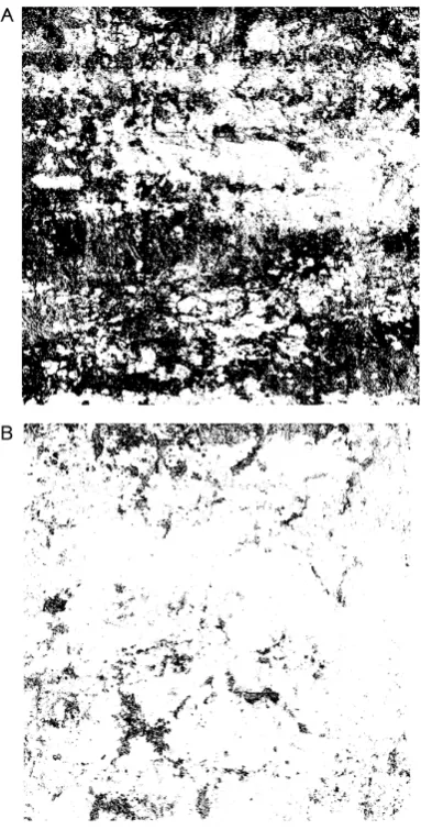
Fig. 1. Images of horizontal sections of 2×2 m corresponding to a depth of: (A) 20 cm and (B) 30 com. Black pixels represent dye stained areas.
The organization of the paper is as follows. First other pa-rameters such as configuration entropy are revisited. Next, a necessary introduction to wavelet transform and singu-larity measures is given as well as a definition of the so-called Wavelet Transform Modulus Maxima (WTMM) (Ma-llat, 1999). The extension to multifractal one dimensional signals is covered next and experiments on soil images are described. Finally some conclusions and future work re-search directions are given.
2 Methodology and previous results
2.1 Dye tracer experiment
The experiments were conducted in a five hectare agricul-tural research site located on the Brazos River floodplain near College Station, Texas. The field in which the plot was
lo-was found, resulting in 15 sections. A 35-mm camera with Kodachrome 60 film was used to photograph each of the hor-izontal sections as they emerged during the excavation. Six-teen sections were photographed: the surface and fifSix-teen sub-surface sections.
The 2×2 m horizontal section at any given depth was re-presented by a matrix of 2048×2048 pixels. Each pixel re-presented an area of approximately 1 mm2. The value of each pixel was either black (dye stained) or white (unstained), so we had two-dimensional binary images like the ones shown in Fig. 1.
2.2 Configuration entropy
Configuration entropy analysis studies the effect of scale in any measure (a scalar quantity that leads to a positive dis-tribution) defined in a plane. If a plane were divided into an arbitrary number of smaller areas (e.g., boxes) and the measure (µ) were estimated in each sub-area, a distribution of the measure would be obtained. Estimation of dye pat-terns from a binary image implies counting pixels represent-ing dyed areas and expressrepresent-ing this count as a percentage of the total number of pixels in the image. We refer to this quan-tity as Dye Tracer percentage (DT) and it is the basis of the configuration entropy.
Mathematically, the probability associated with a case of
j dye pixels in a box of sizeris defined as:
pj(r)=
Nj(r)
n(r) . (3)
whereNj(r) is the number of boxes withj dye pixels and
n(r) is the number of boxes of size r. The configuration entropy is thus defined as:
H (r)= −
r×r
X
j=0
pj(r)log(pj(r)). (4)
H (r)as expresses in Eq. (4) reveals the uncertainty associ-ated with the DT. For proper comparisonH (r)needs to be normalized resulting in:
H∗(r)= H (r) Hmax(r)
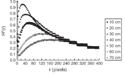
Fig. 2. Normalized configuration entropyH∗(r)versus box sizer from horizontal sections at different depths.
whereHmax(r)=log(r2+1). Plotting the normalized entropy versusrcould be used as a descriptor of the image morphol-ogy. In our experiment, for example, all the horizontal sec-tions showed the same behavior in the configuration entropy curve (Fig. 2). The general pattern was a rapid increase inH
withrfollowed by a gradual decay.
The first point of the curve, forr=1, was totally correlated with the DT of the horizontal section. Note that the decrease in DT with depth was not linear, but showed abrupt changes. By a depth of 15 cm, the DT value had decreased to half of that at the surface, and by 30 cm depth the value was 10%.
3 Wavelets and singularities
3.1 Introduction
Wavelet theory has its origin in several disciplines. The types of functions that are now called wavelets were studied in quantum field theory, signal analysis, and function space theory. In all these areas, wavelet-like algorithms replaced the classical “windowed” Fourier transform.
The windowed Fourier transform serves as means to des-cribe or compare the fine structure of a function at different resolutions. Its basic building blocks are the integer dilates of the sine and cosine functions multiplied by a “window” function. Although quite successful, this method is not ap-plicable to highly localized structures when the window size is fixed.
To overcome these problems, one replaces sine and cosine by a function that has compact support and its dilates and translates form an orthonormal basis of the function space being considered (usuallyL2(R)). The famous Daubechies wavelets (Daubechies, 1992) are an example of these wavelet bases. Other examples, like the derivative of a Gaussian that will be used in our work are also sketched in (Fig. 3)
It can be shown that under certain conditions this type of function performs a multiresolution analysis or decompo-sition of L2(R). Such wavelet decompodecompo-sitions are obtained via a multiresolution analysis (Mallat, 1989). Therefore, the
Fig. 3. Some examples of Wavelet bases: Daubechies of order 4,
first derivative of a gaussian and Mexican Hat wavelets.
main feature we are interested in, is the ability of wavelet transform to focus on localized signal structures performing a multiscale (multiresolution) analysis of signal singularities. Next, we extend this type of analysis to complex signals such as multifractals.
3.2 Wavelet transform and Lipschitz regularity
Conceptually, the continuous wavelet transform (CWT) is a convolution product of a signal with a scaled and translated kernel (usually a n-th derivative of a smoothing kernel in or-der to precisely detect singularities as pointed out later)
Wf (u, s)= 1 s
Z ∞ −∞
f (x)ψ
x−u s
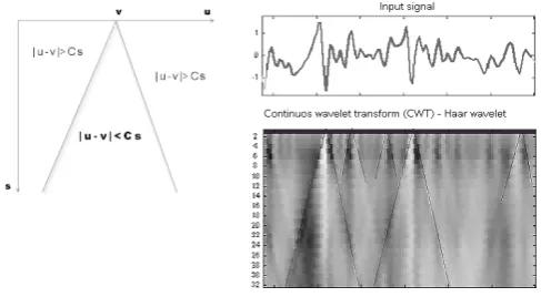
Fig. 4. Cone of influence of and abscissavand example.
To characterize singular structures, Lipschitz exponents are commonly used. They provide uniform regularity mea-surements over time intervals and local measures at any point. If f has a singularity at v, which means that it is not differentiable at this point, the Lipschitz exponent atv
characterizes this singular behaviour.
Proper definitions of Lipschitz exponents are given next: – A functionf is pointwise Lipschitzα≥0 atv if there
existK>0 and a polynomialpvof degreem= bαcsuch
that:
∀t ∈R,|f (t )−pv(t )| ≤k|t−v|α (7)
– A functionf is uniformly Lipschitz αover[a, b]if it satisfies (7) for allv∈[a, b], with a constantK indepen-dent ofv.
To measure the local regularity of a signal is crucial to choose a wavelet with enough vanishing moments. A wavelet func-tionψ (t )is said to haven>αvanishing moments if and only if:
Z ∞ −∞
tkψ (t )dt =0 for 0≤k≤n (8)
It can be shown that a wavelet withn vanishing moments can be written as thent h order derivative of a functionθ, so the resulting wavelet transform is a multiscale differen-tial operator which is able to detect and isolate singularities up to exponentsα≤n, such as the following theorem from establishes.
Theorem (Mallat, 1999)
If f∈L2(R) is uniformly Lipschitz α≤n over [a, b] then there existsA>0 such that:
∀(u, s)∈ [a, b]xR (s >0) |Wf (u, s)≤Asα+ 1 2 (9) Conversely, ifWf (u, s)satisfies Eq. (9) and ifα<nis not an integer thenf is uniformly Lipschitzα on[a+, b−]for any>0.
way, we have to analyze the wavelet transform values inside these cones so that Eq. (9) remains valid as a necessary and sufficient condition for pointwise regularity computation.
As a concluding remark of this section, it must be pointed out that a wavelet able to detect any singularity such as the derivatives of the Gaussian always will be a worse choice than a wavelet fitting the actual range of singularities because the more vanishing moments produce longer effective sup-ports and, as a consequence, coarser estimations.
3.3 Wavelet transform modulus maxima (WTMM) We use the term modulus maximum (strict maximum) to de-scribe any point(u0, s0)such that|Wf (u, s0)|is locally max-imum atu=u0. We call maxima line to any connected curve
s(u)in the scale-space plane(u, s)along which all points are modulus maxima.
It can be shown (Mallat, 1999) that:
– Singularities can be detected finding the abscissa where the wavelet modulus maxima converge at fine scales. – Pointwise regularity (α+1
2) can be calculated by mea-suring the decay slope of log2|Wf (u, s)|as a function of log2(s)at the finest scales. So measuring the decay in the time-scale plane as suggested in Eq. (9) is not ne-cessary. We can control it from its local maxima values connected via the maxima lines.
The Fig. 5 shows a signal with a sharp transition at and its corresponding continuous wavelet transform. We compute the WTMM (Wavelet transform modulus maxima) and store values of the modulus in the maxima lines that converge to the singularity. The decay of the modulus along these maxi-ma lines are given to the right for the ridges numbered as 9,7 and 4 (plotted using continuous, dashed and dotted lines res-pectively). A simple linear regression may be used in order to compute the desired Lipschitz exponents.
3.4 Extension to images
Fig. 5. Wavelet Transform Modulus Maxima and maxima chains.
Fig. 6. Decay of modulus amplitude as function of scale gives Lipschitz exponents.
The extension of the previous concepts to images, or mul-tidimensional signals in general, is conceptually simple, but cumbersome. For the two dimensional case the modulus of the wavelet transform is given by:
Mf (u, v, s)= q
|W1f (u, v, s)|2+ |W2f (u, v, s)|2 (10) withuandvdenoting the two dimensional coordinates and the scale parameter being usually used ass=2j. Now, we compute two separates wavelet transforms:W1refers to the wavelet transform performed along the horizontal dimension andW2refers to the vertical one.
Apart from the modulus, information about the angle is required in order to detect modulus maxima points which are defined as local maxima along the gradient direction which are initially expressed as:
Af (u, v, s)=t an−1 W
2f (u, v, s)
W1f (u, v, s)
!
(11) Next, we show different examples of the results obtained. The CWT has been computed for 20 consecutive scales along
Fig. 7. A 512×512 path of the dye image of the experiment.
Fig. 8. Modulus of the CWT at scales=2.
vertical and horizontal dimensions. The modulus of these images are shown in Fig. 8 fors=2 and in Fig. 9 fors=8. If we extract maxima values we have images like the ones showed in Fig. 10 and in Fig. 11.
4 Wavelets and multifractal analysis
4.1 Multifractal formalism
By multifractal structure we mean that there exists a parti-cular arrangement of the points in an image in the so-called fractal components. Those fractals components are sets de-fined by the property that the image undergoes the same kind of change (transition or singularity) for all the points in the same component.
Fig. 9. Modulus of the CWT at scales=8.
Fig. 10. Modulus maxima of the CWT at scales=2.
That decomposition can be done by means of the wavelet analysis.
First, for each pixelx(u0, v0)its singularity exponent α is computed. Then, all the points in the image are arranged according to the value of their singularity exponent arriving at the well known multifractal spectrumf (α).
4.2 Multifractal spectrum and wavelets
The goal of a multifractal analysis must then be to estimate the singularity distribution. In this context the so called mul-tifractal spectrum and its fractal dimension is used. With the help of the well-known Devil’s staircase fractal we will show how to compute its multifractal spectrum through the wavelet transform.
A Devil’s staircase is the integral of a Cantor measure whose recursive construction implies that the Devil’s stair-case is a self-similar function. Figure 12 displays the devil’s staircase obtained withp1=0.475 andp2=0.525, its wavelet transform computed using the first derivative of a Gaussian and the modulus maxima lines.
Letun(s)the position of all local maxima of the wavelet
modulus transform. The partition function Z measures the
Fig. 11. Modulus maxima of the CWT at scales=8.
Fig. 12. Devil’s staircase, wavelet transform and modulus maxima.
sum at power q of all these wavelet modulus maxima values:
Z(q, s)=X
n
|Wf (un, s)|q (12)
It is important to note that at each scale if there exist more than a maximum in the cone of influence, the sum includes only the maxima of largest amplitude.
For each q (which is a real number) the scaling expo-nent measures the asymptotic decay of the partition function
Z(q, s)at fine scales:
τq =lim s→0
logZ(q, s)
logs (13)
This means thatZ(q, s)∝sτq and intuitively, sinceq has the
Fig. 13. Partition function for several values ofq.
Fig. 14. Moments generating function.
Finally, using the inverse Legendre transform (which is applicable if and only iff (α)is convex) we obtain the mul-tifractal spectrumf (α)as:
f (α)=min
q∈R
q
α+1
2
−τ (q)
(14) wheref (α)is convex when the signal is self-similar (col-loquially speaking a measure is multifractals when its mul-tifractal spectrum exists and has the shape of an inverted parabola). The spectrumf (α)reveals the distribution of sin-gularities in a multifractal multifractal signal which is cru-cial to analyze its properties. The spectrum measures the global repartition of singularities having different Lipschitz regularity. For example, if the signal being considered were monofractal (only one component), the spectrum would con-sist of a single point. In the case of a multifractal as the devil’s staircase or the dye stained images we are working
Fig. 15. f (α)values calculated with Eq. (14) and theoretical spec-trum.
on, the spectrum range of α-values increases according to the increase in the distribution heterogeneity. In conclusion, wider concave spectrum means more heterogeneity.
All these steps applied to the Devil’s staircase example are shown in Fig. 13 whereZ(q, s)are plotted against scale for differentq values. Figure 14 which showτq and finally in
Fig. 15 where values calculated with Eq. (14) and theoretical spectrum (Mallat, 1999) are compared.
Thef (α)spectrum is related to the other commonly used set of multifractal exponents known as generalized fractal di-mensions, calculated from the mass exponent function as:
Dq=
τq
q−1 (15)
The fractal dimension atq=0, equals the geometric support of the measure being studied (equals 1.0 for one dimensional signals or 2.0 for images). The information fractal dimen-sionD1is obtained atq=1 using L’Hopital rule. A value of
D1close to 1.0 characterize a system uniformly distributed throughout all scales, whereasD1close to 0 reflects a subset of the scale in which the irregularities are concentrated. With respect toD2, simply said that is mathematically associated to the correlation function, so it measures the self-similarity of a signal.
For the Devil’s example we haveD1=0.6407 which is near the theoretical value ofD1=log 2log 3=0.6309. One of the rea-sons for the systematic difference between the theoretical and the computed multifractal spectrum might be in the computa-tion ofZ(q, s)=P
n|Wf (un, s)|qwhere at some scales we
may have an indeterminate function forq<0.
5 Multifractal and wavelet based analysis of soil spatial variability
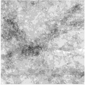
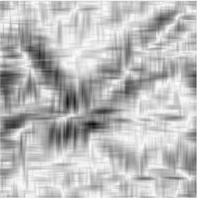
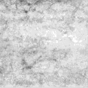
Fig. 16. Dye mass image being processed.
distribution can be uniquely characterized by a single frac-tal dimension (Kravchenko et al., 1999). However, a single fractal dimension might not always be sufficient to represent complex and heterogeneous behaviour of soil spatial varia-tions.
Motivated by this, the work presented in Folorunso et al. (1994) found multifractal parameters to be superior to a sin-gle fractal dimension in distinguishing between soil types. Later Muller (1996) used multifractal analysis to character-ize pore space in chalk and noticed that multifractal proper-ties are closely related to chalk permeability and porosity.
For our application there are two types of experiments. First of all, horizontal sections, such as those of Fig. 1 may be analyzed separately looking for any scaling pattern. Fi-nally the data from all 16 sections were merged to produce a spatial field of two measures: quantity of dye tracer (dye mass) and maximum dye infiltration depth (dye depth). The dye mass image is shown in Fig. 16 where darker values rep-resent higher dye mass. Although, initially dye mass and dye depth quantities are integers in the range 0 to 16 (the same value as number of sections) proper normalization is needed in order to accurately compute power-law relationships be-tween quantities and box size. For this reason the sum of all values is equalled to 1 prior to any computation.
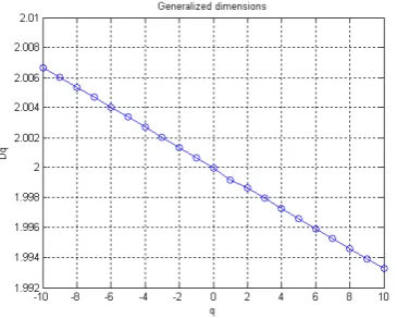
5.1 Box-counting methods for multifractal analysis A detailed description of the box-counting algorithm applied to our case study can be found in Tarquis et al. (2006), so only some results are given in order to analyze how wavelet anal-ysis can complement box-counting algorithms. Figure 17 shows the resulting bi-log plots of the partition function ver-sus box-size for different horizontal planes (only those cor-responding to 20 cm and 30 cm are given). Partition function and generalized dimension for different values ofqare given in Figs. 18 and 19 for the dye-mass image.
Fig. 17. Bi-log plot of partition function versus box-size for
differ-ent sections: (A) 20 cm and (B) 30 cm.
All partition functions showed a clear pattern in the data with two distinctive areas. One where there was a linear re-lationship and another where the slope was almost constant. So, only when the box-size passed a certain value a scaling pattern begins.
5.2 Wavelet analysys (WTA)
Fig. 18. Bi-log plot of partition function versus box-size for dye
mass image.
Fig. 19. Generalized fractal dimension for the dye mass image.
occurs only for scales larger thans≥8, so maxima lines re-vealing that scaling pattern do not propagate adequately.
However analysis of Lipschitz exponents along maxima lines is still convenient for our analysis providing important information about distribution of singularities (and so, the
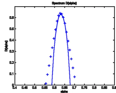
f (α)spectrum). As suggested in Zhong and Ning (2005) and Struzik (1999) it is possible to evaluate singular spectrum lo-cally using Eq. (9) and tracing an histogram of the number of pixels within a certain interval ofαvalues. First results for the dye mass image along the scales where a multifractal behaviour is expected are given in Fig. 20 where the centroid of the histogram equals α0=1.77, approximately equal to the computed value with box-counting method which equals
α0=1.83.
Fig. 20. Histogram of Local Lipschitz exponents for the dye mass
image.
6 Conclusions
The application of the CWT (Continuos wavelet transform) and its particular representation called WTMM (Wavelet transform modulus maxima) to multifractal analysis has al-most reached the status of a standard in natural phenomena analysis contributing to substantial progress in each domain where it has been applied.
This paper reviews the main concepts involved in the mul-tifractal formalism and its relation with the signal represen-tation obtained using the wavelet transform. The selected domain of application has been Hydrology, where different authors relate the permeability of different materials to the multifractal spectrum.
Some experiments using a dye tracer over a clay soil has been done, mainly focusing on the multifractal spectrum of the dye mass and dye depth quantities. Previous results by some of the authors (Tarquis et al., 2006) related with other parameters such as configuration entropy are also revisited trying to provide a complete set of measures capable of char-acterize soil properties.
Classical multifractal characterization with box-counting methods are given both for each horizontal section and for the dye mass image which shows that only for larger scales a multifractal behavior is expected. This is the main rea-son behind unexpected results obtained with wavelet exten-sion of methods exposed in Sect. 4. However, if we plot an histogram of coefficientsα for selected scales we obtain a very good approximation of the multifractal spectrum with the advantage that we precisely know the location of diffe-rentα-Lipschitz exponents. This may be an important and complementary information.
Arneodo, A., Grasseau, G., and Holshneider, M.: Wavelet transform of multifractals, Phys. Rev. Lett., 61, 2281–2284, 1988. Arneodo, A., Bacry, E., and Muzy, J.: Solving the inverse fractal
problem from wavelet analysis, Europhysics Lett., 25(7), 479– 484, 1994.
Daubechies, I.: Ten lectures on wavelets, volume 61, CBMS con-ference on wavelets, 1992.
Folorunso, O. A., Puente, D. E., Rolston, D. E., and Pinzon, J. E.: Statistical and fractal evaluation of the spatial characteristics of soil surface strength, Soil Sci. Soc. Am. J., 58, 284–295, 1994. Hsung, T., Lun, D., and Siu, W.: Denoising by singularity detection,
IEEE Trans. Signal Processing, 47, 3139–3144, 1999.
Kravchenko, A. N., Boast, C. W., and Bullock, D. G.: Multifractal analysis of soil spatial variability, Agronomy J., 91, 1033–1041, 1999.
fractal Sierpinsky carpets: Theory and application to upscaling effective saturated hydraulic conductivity, Geoderma, 134, 240– 252, 2006.
Struzik, Z. R.: Direct multifractal spectrum calculation from the wavelet transform. Technical Report INS-R9914, Information Systems, ISSN: 1386-3681, Amsterdam, 1999.
Tarquis, A. M., McInnes, K., Keys, J., Saa, A., Garcia, M. R., and Diaz, M. C.: Multiscaling analysis in a structured clay soil using 2D images, J. Hydrol., 322, 236–246, 2006.