Two-dimensional reconstruction of past sea level (1950–2003) from
tide gauge data and an Ocean General Circulation Model
W. Llovel1, A. Cazenave1, P. Rogel2, A. Lombard3, and M. B. Nguyen1 1LEGOS, OMP, 18 avenue Edouard Belin, 31401 Toulouse Cedex 09, France
2CERFACS/URA1875, 42, Avenue Gaspard Coriolis, 31057 Toulouse Cedex 01, France 3CNES, 18 avenue Edouard Belin, 31401 Toulouse Cedex 09, France
Received: 20 February 2009 – Published in Clim. Past Discuss.: 20 March 2009 Revised: 18 May 2009 – Accepted: 2 June 2009 – Published: 23 June 2009
Abstract. A two-dimensional reconstruction of past sea level is proposed at yearly interval over the period 1950– 2003 using tide gauge records from 99 selected sites and 44-year long (1960–2003) 2◦×2◦ sea level grids from the
OPA/NEMO ocean general circulation model with data as-similation. We focus on the regional variability and do not attempt to compute the global mean trend. An Empirical Orthogonal Function decomposition of the reconstructed sea level grids over 1950–2003 displays leading modes that re-flect two main components: (1) a long-term (multi-decadal), regionally variable signal and (2) an interannual, region-ally variable signal dominated by the signature of El Nino-Southern Oscillation. Tests show that spatial trend patterns of the 54-year long reconstructed sea level significantly de-pend on the temporal length of the two-dimensional sea level signal used for the reconstruction (i.e., the length of the gridded OPA/NEMO sea level time series). On the other hand, interannual variability is well reconstructed, even when only∼10-years of model grids are used. The robustness of the results is assessed, leaving out successively each of the 99 tide gauges used for the reconstruction and comparing observed and reconstructed time series at the non considered tide gauge site. The reconstruction performs well at most tide gauges, especially at interannual frequency.
1 Introduction
Sea level is an indicator of climate change because it inte-grates the response of many components of the Earth
sys-Correspondence to: W. Llovel ([email protected])
tem: the ocean and its interaction with the atmosphere, land ice, terrestrial waters. Even the solid Earth has some im-pact on sea level. Since the beginning of the 1990s, sea level is precisely measured by satellite altimetry systems (i.e., Topex/Poseidon, Jason-1 and now Jason-2) with global coverage and short revisit time. The satellite observations have revealed that sea level does not rise uniformly: some re-gions rise faster than the global mean; in some other rere-gions sea level rise slower (Bindoff et al., 2007). It has been shown that the main cause of regional variability in rates of sea level change is non uniform thermal expansion of the oceans (Ca-banes et al., 2001), although other processes may also give rise to regional sea level trends (e.g., the solid Earth response to last deglaciation and gravitational effects of on-going land ice melt). Studies have established that trend patterns in ther-mal expansion fluctuate both in space and time in response to ENSO (El Nino-Southern Oscillation), NAO (North Atlantic Oscillation) and PDO (Pacific Decadal Oscillation) (Lom-bard et al., 2005). Thus, it is important to know past regional variability and see how it evolves with time. Climate model projections suggest significant regional variability with re-spect to the global sea level rise for the end of this century (Meehl et al., 2007). But account for the interannual/decadal variability associated with ENSO and other phenomena by coupled climate models is still imperfect insight into past re-gional variability over time spans longer than the altimetry record may be helpful to improve the climate models.
Unfortunately, for the last century, information about sea level is sparse and essentially based on tide gauge records along islands and continental coastlines. This data set can-not alone inform on open ocean regional variability. For that reason, a number of previous studies have attempted to re-construct past decades sea level in two dimensions (2-D), combining sparse but long tide gauge records with global
218 W. Llovel et al.: Two-dimensional reconstruction of past sea level (1950–2003) gridded (i.e., 2-D) sea level (or sea level proxies) time series
of limited temporal coverage (Chambers et al., 2002; Church et al., 2004; Berge-Nguyen et al., 2008). The present study has a similar objective: it expands an earlier work by Berg´e-Nguyen et al. (2008) (hereafter denoted as BN08) but makes use of different information for the 2-D fields used for the reconstruction. Previous studies used global sea level grids based on Topex/Poseidon satellite altimetry of limited (10 to 15 years) temporal coverage (e.g., Chambers et al., 2002; Church et al., 2004) or long but spatially inhomogeneous gridded time series of thermal expansion based on in situ hy-drographic data (e.g., BN08). In this study, we use global dynamic heights grids from an Ocean General Circulation Model (OGCM), the OPA/NEMO model constrained by data assimilation (Madec et al., 1998). These model outputs, available over a 46-year time span (1960–2005), are com-bined with tide gauge records (that cover the period 1950– 2003). We consider 44-year (1960–2003) time span for the OPA/NEMO outputs to be in line with the tide gauge records length (that ends in 2003). The advantage of using such a long 2-D data set is twofold: (1) the 44-year long coverage minimizes the probably non stationarity of altimetry-based spatial patterns (see BN08 for a discussion), (2) the combi-nation of model-data resulting from an assimilation approach solves the problem of poor geographical and deep ocean cov-erage of in situ hydrographic data. The resulting sea level re-construction is presented below for the 1950–2003 time span.
2 Method
Several studies have developed methods for reconstructing past time series of oceanographic (e.g., sea surface tempera-ture, sea surface height) or atmospheric (e.g., surface wind speed, surface pressure) fields by combining 2-D grids of limited temporal coverage (in general available from remote sensing observations over the last 2 decades or less) with historical (several decade-long), sparse 1-D records (e.g., Smith et al., 1994, 1996; Kaplan et al., 1997, 1998, 2000; Church et al., 2004, 2006; Chambers et al., 2002; Beckers and Rixen, 2003; Alvera-Azcarate et al., 2005; Rayner et al., 2003). The general approach uses Empirical Orthogonal Em-pirical Functions (EOF) decomposition (e.g., Preisendorfer, 1988) of the 2-D time series to extract the dominant modes of spatial variability of the signal. These EOF spatial modes are then fitted to the 1-D records to provide reconstructed multidecade-long 2-D fields. Different computational vari-ants of the method have been developed to estimate the re-constructed long-term 2-D fields depending on the use of a priori information and data errors (e.g., Kaplan et al., 2000; Rayner et al., 2003; Church et al., 2004) or not (Smith et al., 1996). When applied to long-term past reconstruction, an implicit assumption of the method is the temporal station-arity of the spatial patterns recovered from the EOF modes of the short-term 2-D fields. The spatial covariance obtained
from the 2-D fields must indeed be able to describe the spa-tial covariance over the entire period of the reconstruction (e.g., Smith et al., 1996). If the dominant modes of spa-tial variability have characteristic time scales longer than the time interval covered by the 2-D fields, EOF spatial modes may incompletely capture the relevant long-term signal. In particular the multi-decadal components of the reconstructed signal may be in error.
We briefly summarize below the methodology. Let us call Fo(x,y,t) and Go(x,y,t) observed global gridded short-term fields and sparse, incomplete long-term sea level data re-spectively, withx,y andt being Cartesian coordinates and time. The time span Tf covered by the Fo(x,y,t) fields is
basically shorter than that -called Tg- of the reconstructed fields. Here, Fo(x,y,t) corresponds to gridded sea level from the OPA/NEMO models over 1960–2003, while the Go(x,y,t) -spatially incomplete- fields correspond to tide gauge records over 1950–2003. The Fo(x,y,t) function is expressed as a sum of combinedXn(x,y) spatial modes anden(t) principal
com-ponents using an EOF decomposition (with zero global mean trend). The objective of the reconstruction is to compute 2-D Go(x,y,t) fields with global spatial coverage – hereafter denoted as GR(x,y,t) – over the Tg time span (here 1950–
2003). The 2-D reconstructed sea level fields are written as GR(x,y,t)=P[Xn(x, y) Yn(t)] whereYn(t) are new
prin-cipal components computed at each time stept and mode n, through a least-squares fit that minimizes the quantityε expressed by ε=[Go(x,y,t)−P
[Xn(x, y)Yn(t)]]2. For more
details, see BN08.
3 Tide gauge data
W. Llovel et al.: Two-dimensional reconstruction of past sea level (1950–2003) 219 16
Figure 1
Figure 2a
Fig. 1. Location map of the 99 tide gauges (open circles) used in this
study. Stars correspond to the comparison sites with records shown in Fig. 10. The background map shows the OPA/NEMO spatial sea level trends computed over 1960–2003 (in mm/yr).
gauge records is that measurements are made in local datum that varies from one site to another. By working with the derivatives, this problem can be overcome (e.g., Holgate and Woodworth, 2004; Holgate, 2007). Here we choose a differ-ent approach (e.g., Kuo et al., 2008) consisting of subtracting from each sea level record a mean value computed over the 1950–2003 time span (note that the 99 tide gauge records are almost complete; when small gaps,<3 years, are observed, we linearly interpolate missing data). Figure 1 shows the distribution of the tide gauge sites used in this study (super-imposed on a map of OPA/NEMO dynamic height spatial trends).
4 OPA/NEMO Ocean General Circulation Model outputs
The ocean reanalysis used in this study has been produced with a 3-dimensional variational assimilation system (Daget and Weaver, 2008) applied to the OPA/NEMO OGCM (Madec et al., 1998). The model resolution, 2◦on average, with a latitudinal refinement in the tropics, is coarse but ap-propriate for the multidecadal period of interest here. The model is forced by the standard reanalyse ERA40 heat fluxes (Uppala et al., 2005) and corrected water fluxes (Troccoli and Kalberg, 2004). From September 2002 onwards, when ERA40 terminates, ECMWF (European Centre for Meteoro-logical Forecast) operational surface fluxes are used as forc-ing. The assimilation system minimizes the discrepancy be-tween model and observations by constraining the model to remain close to the a priori model state. In this iterative pro-cedure, the distance to the observations (respectively to the model state) is taken as the norm defined by the observation error (respectively the model state error). Whilst the obser-vational error is straightforward to characterise, a lot of work has been done to properly define the model state error (Ricci
(a)
Figure 1
Figure 2a
(b)
17
Figure 2b
Figure 3a
Fig. 2. (a) Spatial trend map over 1950–2003 of reconstructed sea
level (with 10 modes for the reconstruction); nominal case (case 1).
(b) Same as (a) but with 20 modes for the reconstruction. Unit:
mm/yr.
et al., 2005; Weaver et al., 2006). This ensures the propa-gation of information to the model variables not directly ob-served (e.g., sea level and velocity) and hence the realism of the analyses. Quality controlled temperature and salin-ity profiles from the EN3 oceanographic data base (Ingelby and Huddleston, 2007) are assimilated every 10 days from January 1960 to December 2006. Note that these profiles were not corrected for the recently discovered instrumenta-tion problems. The model outputs are on a monthly basis but only annual averages are considered hereafter.
As described in Roullet and Madec (2000), the model is formulated with a prognostic free surface, constant volume and salt preserving scheme, assuming that the mean sea level does not vary. Hence, both forcing and data assimilation have been designed to ensure that no drift in the mean sea level occurs. Water flux balance between precipitation, evapora-tion and runoff is set to zero in the free surface equaevapora-tion, and assimilation increments (i.e., the model corrections applied every 10 days to the model using temperature and salinity observations) are built under the constraint that the sea level increment is zero on global average. In addition, the model is
220 W. Llovel et al.: Two-dimensional reconstruction of past sea level (1950–2003)
(a)
17
Figure 2b
Figure 3a
(b)
18
Figure 3b
Figure 3c
(c)
-90 -60 -30 0 30 60 90
0 120 240 360
-90 -60 -30 0 30 60 90
0 60 120 180 240 300 360
-7 -5 -3 -1 1 3 5 7
mm/year
(d)
Fig. 3. Spatial trend map over 1950–2003 of reconstructed sea level. (a) spatial EOFs from OPA/NEMO over 1973–2003 (case 2); (b)
spatial EOFs from OPA/NEMO over 1983–2003 (case 3); (c) spatial EOFs from OPA/NEMO over 1993–2003 (case 4); (d) spatial EOFs from Topex/Poseidon altimetry (case 5). Unit: mm/yr.
relaxed towards a climatology (Levitus et al., 1994) poleward of 60◦and in the semi-enclosed seas, so that interannual vari-ations in those regions are almost suppressed. On the other hand, no constraint is applied over open ocean areas.
In Fig. 1 are displayed sea level trends from the OPA/NEMO model with data assimilation over 1960–2003. For the reasons explained above, the map has zero global mean (uniform) trend. Important regional variability is ob-served, especially in the western parts of the basins. The strongest spatial patterns are located close to the western boundary currents (e.g., Gulf Stream in the Northwestern At-lantic, Kuroshio in the Northwestern Pacific; Malvinas Cur-rent in the Southwestern Atlantic).
Here we focus on the regional variation and do not attempt to reconstruct the global mean trend. However, we must pay attention on a possible contamination of any global mean trend to the reconstructed sea level. We first checked that the model EOFs have zero global mean trend (this is expected as the model does not contain any uniform trend signal). We further checked that EOFs of the reconstruction do not con-tain either significant non-zero global average.
5 Sea level reconstruction
5.1 Reconstructed spatial trend patterns over 1950–2003
We reconstructed 2-D sea level grids at yearly interval over 1950–2003 combining spatial EOFs of the OPA/NEMO grids over 1960–2003 (44 years of gridded data) with 99 tide gauge time series covering the 1950–2003 time span. Most of the variance of the reconstructed sea level is included in the first 10–20 modes. Highest-order modes exhibit essentially noise. In the following, we consider as nominal case (called case 1), the first 10 modes when reconstructing sea level (with 75% of the total signal variance). Corresponding reconstructed spatial trend map over 1950–2003 is presented in Fig. 2a. We note that trend amplitudes are everywhere higher than in the model trend map (Fig. 1) but extrema are located in the same regions (e.g., Gulf Stream, Kuroshio; Malvinas Current, etc.). For comparison we also show the spatial trend map with the first 20 modes used for the reconstruc-tion (Fig. 2b). The 20 modes case contains more energy but is also noisier (as discussed in BN08).
W. Llovel et al.: Two-dimensional reconstruction of past sea level (1950–2003)Figure 3d 221
Figure 4a
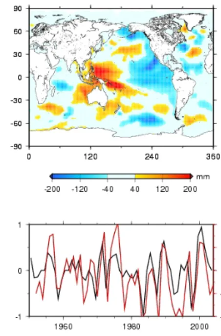
Fig. 4a. EOF decomposition over 1950-2003 for nominal case (case 1): left: mode 1; right mode 2 (with SOI index is superimposed on the
temporal curve).
20
Figure 4b
Figure 4c
Fig. 4b. Same as (a) but for case 2.
-case 3-, and 11 years of OPA/NEMO grids (1993–2003) -case 4. Case 4 can be compared with studies that use decade-long Topex/Poseidon altimetry grids for sea level re-construction (e.g., Chambers et al., 2002; Church et al., 2004). Corresponding reconstructed spatial trend maps are presented in Fig. 3a, b, c (using for each case, the num-ber of modes that correspond to 75% of the total variance). Significant regional differences are noticed between the first
two cases (44 years and 31 years of OPA/NEMO grids, re-spectively) and cases 3 and 4 (21 years and 11 years of OPA/NEMO grids, respectively) , in particular in the North Atlantic, Indian and Austral oceans, and Northeast Pacific. Spatial trend patterns for cases 1 and 2 give are quite in agreement. A similar observation can be done for cases 3 and 4. We thus observe a transition in reconstructed trends when the temporal coverage of OPA/NEMO grids increases
222 W. Llovel et al.: Two-dimensional reconstruction of past sea level (1950–2003) 20
Figure 4b
Figure 4c
Fig. 4c. Same as (a) but for case 3.
21
Figure 4d
Fig. 4d. Same as (a) but for case 4.
from∼20 years to∼30 years. As discussed below, the low-frequency sea level signal may not be well captured in cases that use short spatial grids for the reconstruction (cases 3 to 5). In the latter cases, patterns representing interannual variability dominate the reconstructed spatial trends.
To compare with case 4, we also show in Fig.3d recon-structed sea level trends (over 1950–2003) using 11 years (1993–2003) of Topex/Poseidon sea level grids (case 5). The
W. Llovel et al.: Two-dimensional reconstruction of past sea level (1950–2003) 223
22
Figure 5
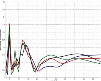
Fig. 5. Energy spectrum of the interannual variability for cases 1
(blue), 4 (red) and 5 (green) and SOI index (black).
We performed EOF decompositions of the reconstructed sea level grids over 1950–2003 for cases 1 to 4. Figure 4 a, b, c, d shows the two leading EOF modes each case. Mode 1 temporal curve (principal component) of nominal case is dominated by a positive slope. Associated mode 1 spatial map closely resembles case 1 reconstructed trend map (Fig. 2), with strong signal in the Austral Ocean (especially southeast of Africa). This suggests that the reconstructed trend map for the nominal case mostly reflects a long-term (multi-decadal), regionally variable signal. Mode 2 of case 1 (Fig. 4a right panel) is dominated by the interannual vari-ability, and displays clear signature of ENSO in the tropi-cal Pacific: the Southern Oscillation Index (SOI) -a proxy of ENSO- is significantly correlated (61%) to the temporal curve on which is it superimposed. It is worth mentioning that the spatial map of mode 2 (case 1) is very similar to the satellite altimetry-based sea level trend map over 1993– 2003 (see below). Hence, whilst mode 1 reflects long-term, multidecadal signal, mode 2 mostly reflects ENSO-type in-terannual variability.
The two leading modes of case 2 (Fig. 4b) closely resem-ble those of case 1. The first EOF mode of cases 3 and 4 reflects interannual variability (as mode 2 of cases 1 and 2). This is illustrated in Fig. 5 which shows energy spectra of the interannual signal for cases 1, 4 and 5 (i.e., temporal curves spectra of corresponding EOF modes). SOI spectrum is su-perimposed. The agreement between the four curves is strik-ing. Peaks in the 3–5 yr and 10–15 yr wavebands dominate. They mainly reflect ENSO frequency and associated decadal modulation. On the other hand, looking at the long-term sig-nal (e.g., comparing modes 1 of case 1 and 2 with mode 2 of cases 3 and 4), we note significant difference in the spa-tial maps, suggesting that multidecadal fluctuations are only partly recovered when using short-term gridded time series for the reconstruction (e.g., cases 3 and 4).
(a)
Figure 6a
Figure 6b (b)
Figure 6a
Figure 6b
Fig. 6. Spatial sea level trend map over 1993–2003. (a)
recon-structed sea level for nominal case. (b) observed sea level trends from satellite altimetry (uniform trend removed). Unit: mm/yr.
5.2 Robustness of the reconstruction
5.2.1 Sea level reconstruction over the altimetry (1993– 2003) period using the OPA/NEMO EOFs A way to check the validity of the reconstruction is to look at the reconstructed sea level trends over the altimetry period (here 1993–2003) for which we trust the spatial trend pat-terns. Figure 6a shows the reconstructed spatial trend map over 1993–2003 based on 44-years of OPA/NEMO grids. Comparing with Fig. 6b which shows observed satellite al-timetry spatial trend map over 1993–2003 (uniform trend re-moved) indicate very good agreement, although the recon-structed map is smoother (as expected considering the low resolution of the OPA/NEMO model).
5.2.2 Cross-validation of reconstructed series and tide gauge records
Another way to check the robustness of the reconstruction consists of reconstructing sea level, leaving out successively each one of the 99 tide gauge records (thus each of these 99 reconstructions now uses a set of 98 tide gauges, with
224 W. Llovel et al.: Two-dimensional reconstruction of past sea level (1950–2003)
24
Figure 7a
Figure 7b
Fig. 7a. Subset of 18 tide gauges not used in the reconstruction; observed record (solid curve); reconstructed sea level curve (thin dotted
curve).
24
Figure 7a
Figure 7b
Figure 8a
figure 8b Figure 8a
figure 8b
Fig. 8. Histogram of detrended sea level rms differences at the
99 tide gauges (reconstructed minus observed); Upper: case 1; Lower case 5 (reconstruction with Topex/Poseidon). Unit: mm.
different distribution from one case to another). For each deleted tide gauge, we compare the reconstructed sea level time series at the tide gauge site with the PSMSL data (re-constructed sea level is averaged within 2◦around the tide gauge site). For this test we consider two cases: case 1 (re-construction with 44 years of gridded OPA/NEMO grids) and case 5 (reconstruction with 11 years of Topex/Poseidon grid-ded data). Figure 7a shows a subset of 18 comparisons (cor-responding site locations are enhanced by stars in Fig. 1). Figure 7b is similar to Fig. 7a except for the trend which has been removed. We note that in general interannual to decadal variability is well reproduced (Fig. 7b). The average correla-tion at the 99 sites amounts to∼60%. The trends also agree well in most cases, although not everywhere. Sites where trends disagree concern mostly northeast Atlantic areas (e.g., North Shields, Lowestoft, Santander, La Coruna, and Vigo). We suspect that this is due to local underestimated variability in the OPA/NEMO reanalysis, especially in the first 20 years of the period. Similar test performed for case 5 (not shown) shows very similar results for the detrended time series.
Figure 9a
Figure 9b Figure 9a
Figure 9b
Fig. 9. Reconstructed sea level trends at the 99 tide gauges as a
function of observed trends. Upper: case 1; Lower: case 5 (recon-struction with Topex/Poseidon). Unit: mm/yr.
To see the above results in another way, we have com-puted the root mean squared (rms) differences between re-constructed and observed (detrended) sea level time series as well as between trends. Corresponding histograms for the cases 1 and 5 are shown in Fig. 8. Rms (detrended) sea level differences are included in the 15–60 mm but histogram for case 1 is more spread than for case 5. Figure 9 shows plots of reconstructed sea level trends at the 99 tide gauges as a function of observed trends for the two cases (cases 1 and 5). Here we see that case 1 gives better results than case 5, with higher correlation. These comparisons indicate that the re-construction performs well at the interannual time scale (as previously found by Chambers et al., 2002 and Church et al., 2004), with better results for case 5 than case 1. On the other hand, case 1 gives much better results for the trends (hence at multidecadal time scale) than case 5.
226 W. Llovel et al.: Two-dimensional reconstruction of past sea level (1950–2003) 6 Conclusions
We have performed a new 2-D sea level reconstruction over 1950–2003. The main change compared to previous pub-lished results (e.g., Chambers et al., 2002; Church et al., 2004; Berge-Nguyen et al., 2008) is the use of 44-year long gridded sea level data set from the OPA/NEMO OGCM with assimilation. This allows us to compute spatial EOFs over a >40 yr time span, long enough to capture the multidecadal variability in regional sea level (in addition to the interan-nual variability). Hopefully, this may prevent from problems due to the use of short-term altimetry grids. Another advan-tage is the good spatial sampling of the OPA/NEMO out-puts compared to in situ-based thermal expansion data (as in BN08). The main conclusion of this study is that using spatial EOFs computed over a short time span (e.g.,∼10– 20 years) leads to 2-D reconstructed trend patterns signifi-cantly different than when 40 years of EOFs are used. The latter case, not only captures the interannual variability (re-lated to ENSO and possibly NAO and PDO) but also the multidecadal variability. Even if they have local deficiencies, such 2-D reconstructed sea level time series based on low res-olution ocean reanalysis are able to bring physically consis-tent large-scale, low-frequency patterns associated with ma-jor climatic modes of variability.
As a final remark, we think that the use of OGCM outputs is a step towards better reconstruction of long-term sea level time series (at least waiting for global multidecadal altime-try records). Future improvements is expected by using new generation of eddy-permitting OGCM outputs with higher spatial resolution (e.g., 0.25◦×0.25◦) in which some local
misbehaviors can be corrected. This would provide finer de-scription of the spatial trend patterns. Progress in this direc-tion is already underway.
Acknowledgements. We thank Don Chambers, C. K. Shum and an anonymous reviewer for very useful comments.
Nicolas Daget and A. T. Weaver are thanked for their provision of the ocean reanalysis data. These data were produced for the EU FP6 Integrated Project ENSEMBLES (Contract number 505539), whose support is gratefully acknowledged. William Llovel PhD grant is supported by CNRS and Region Midi-Pyrenees.
Edited by: V. Masson-Delmotte
The publication of this article is financed by CNRS-INSU.Ł
References
Alvera-Azcarate, A., Barth, A., Rixen, M., and Beckers, J. M.: Reconstruction of incomplete oceanographic data sets us-ing empirical orthogonal functions: applications to the Adri-atic sea surface temperature, Ocean Model, 9(4), 325–346, doi:10.1016/j.ocemod.2004.08.001, 2005.
Berge-Nguyen, M., Cazenave, A., Lombard, A., Llovel, W., Viarre, J., and Cretaux, J. F.: Reconstruction of past decades sea level using thermosteric sea level, tide gauge, satellite altimetry and ocean reanalysis data, Global. Planet. Change, 62, 1–13, 2008. Bindoff, N., Willebrand, J., Artale, V. , Cazenave, A., Gregory, J.,
Gulev, S., Hanawa, K., Le Qu´er´e, C., Levitus, S., Nojiri, Y., Shum, C. K., Talley, L., and Unnikrishnan, A.: Observations: oceanic climate and sea level, in: Climate change 2007: The physical Science Basis. Contribution of Working Group I to the Fourth Assessment report of the Intergouvernmental Panel on Climate Change, edited by: Solomon S., Qin, D., Manning, M., Chen, Z., Marquis, M., Averyt, K. B., Tignor, M., and Miller, H. L., Cambridge University Press, Cambridge, UK, and New York, USA, 385–428, 2007.
Cabanes, C., Cazenave, A., and Le Provost, C.: Sea level rise during past 40 years determined from satellite and in situ observations, Science, 294, 840–842, 2001.
Cazenave A. and Nerem R. S.: Present-day sea level change: ob-servations and causes, Rev. Geophys., 42, RG3001, doi:8755-1209/04/2003RG000139, 2004.
Chambers, D. P., Mehlha, C. A., Urban, T. J., and Nerem, R. S.: Analysis of interannual and low-frequency variability in global mean sea level from altimetry and tide gauges, Phys. Chem. Earth, 27, 1407–1411, 2002.
Church, J. A., White, N. J., Coleman, R., Lambeck, K., and Mitro-vica, J. X.: Estimates of the regional distribution of sea-level rise over the 1950 to 2000 period, J. Climate, 17(13), 2609–2625, 2004.
Church, J. A., White, N. J., and Hunter, J. R.: Sea-level rise at tropical Pacific and Indian Ocean islands, Global Planet. Change, 53(3), 155–168, 2006.
Daget, N., Weaver, A. T., and Balmaseda, M. A.: Ensemble estima-tion of background-error variances in a three-dimensional varia-tional data assimilation system for the global ocean, Q. J. Roy. Meteorol. Soc., 135, 1071–1094, 2009.
Holgate, S. J. and Woodworth, P. L.: Evidence for enhenced coastal sea level rise during the 1990s, Geophys. Res. Lett., 31, L07305, doi:10.1029/2004GL019626, 2004.
Holgate, S. J.: On the decadal rates of sea level change dur-ing the twentieth century, Geophys. Res. Lett., 31, L01602, doi:10.1029/2006GL028492, 2007.
Ingleby, B. and Huddleston, M.: Quality control of ocean temper-ature and salinity profiles – historical and real-time data, J. Mar. Sys., 65, 148–175, 2007.
Kalnay, E, Kanamitsu, M., Kistler, R., Collins, W., Deaven, D., Gandin, L., Iredell, M., Saha, S., White, G., Woollen, J., Zhu, Y., Leetmaa, A., Reynolds, B., Chelliah, M., Ebisuzaki, W., Higgins, W., Janowiak, J., Mo, K. C., Ropelewski, C., Wang, J., Roy, J., and Joseph, D.: The NCEP/NCAR 40-year reanalysis project, B. Am. Meteorol. Soc., 77, 437–471, 1996.
doi:10.3319/TAO.2008.19.1-2.21.(SA), 2008.
Levitus, S., Burgett, R., and Boyer, T. P.: World Ocean Atlas (Na-tional Oceanic and Atmospheric Administration, Silver Spring, MD), Vols. 3 and 4, 1994.
Lombard, A., Cazenave, A., Le Traon, P. Y., and Ishii, M.: Contri-bution of thermal expansion to present-day sea level rise revis-ited, Global Planet. Change, 47, 1–16, 2005.
Madec, G., Delecluse, P., Imbard, M., and Levy, C.: OPA 8.1 Ocean General Circulation Model reference manual. Notes du pˆole de mod´elisation, Institut Pierre Simon Laplace (IPSL), France, 1998.
Meehl, G. A., Stocker, T. F., Collins, W. D., Friedlingstein, P., Gaye, A. T., Gregory, J. M., Kitoh, A., Knutti, R., Murphy, J. M., Noda, A., Raper, S. C. B., Watterson, I. G., Weaver, A. J., and Zhao, Z.-C.: Global Climate Projections, in: Climate Change 2007: The Physical Science Basis. Contribution of Working Group I to the Fourth Assessment Report of the Intergovernmental Panel on Climate Change, edited by: Solomon, S., Qin, D., Manning, M., Chen, Z., Marquis, M., Averyt, K. B., Tignor, M., and Miller, H. L., Cambridge University Press, Cambridge, United Kingdom and New York, NY, USA, 2007.
Peltier, W. R.: Global Glacial Isostasy and the Surface of the Ice-Age Earth: The ICE-5G (VM2) Model and GRACE, Annu. Rev. Earth Pl. Sc., 32, 111–149, 2004.
Preisendorfer, R. W.: Principal component Analysis in Meteorol-ogy and Oceanography, Developments in Atmospheric Science, vol. 17, Elsevier, 425 pp., 1988.
Rayner, N. A., Parker, D. E., Horton, E. B., Foll, C. K., Alexer, L. V., Powell, D. P., Kent, E. C., and Kaplan, A.: Global analyses of SST, sea ice, and night marine air temperature since the late nineteenth century, J. Geophys. Res., 108, 4407, doi:10.1029/2002JD002670, 2003.
tion, Mon. Weather Rev., 133, 317–338, 2005.
Roullet, G. and Madec, G.: Salt conservation, free surface and vary-ing volume : a new formulation for Ocean GCMs, J. Geophys. Res., 105, 23927–23942, 2000.
Smith, T. M., Reynolds, R. W., and Ropelewski, C. F.: Optimal averaging of seasonal sea surface temperatures and associated confidence intervals (1860–1989), J. Climate, 7, 949–964, 1994. Smith, T. M., Reynolds, R. W., Livezey, R. E., and Stockes, D.: Reconstruction of historical sea surface temperature using Em-pirical Orthogonal Functions, J. Climate, 9, 1403–1420, 1996. Toumazou, V. and Cretaux, J. F.: Using a Lanczos eigensolver in the
computation of Empirical Orthogonal Functions, Mon. Weather Rev., 129, 1243–1250, 2001.
Troccoli, A. and Kallberg, P.: Precipitation correction in the ERA-40 reanalysis, ERA-ERA-40 Project Report Series 13, ECMWF, 2004. Uppala, S. M., da Costa Bechtold, V., Fiorino, M., Gibson, J. K., Haseler, J., Hernandez, A., Kelly, G. A., Li, X., Onogi, K., Saari-nen, S., Sokka, N., Allan, R. P., Andersson, E., Arpe, K., Bal-maseda, M. A., Beljaars, A. C. M., van de Berg, L., Bidlot, J., Bormann, N., Caires, S., Chevallier, F., Dethof, A., Dragosavac, M., Fisher, L., Fuentes, M., Hagemann, S., H´olm, E., Hoskins, B. J., Isaksen, L., Janssen, P. A. E. M., Jenne, R., McNally, A. P., Mahfouf, J.-F., Morcrette, J. J., Rayner, N. A., Saunders, R. W., Simon, P., Sterl, A., Trenberth, K. E., Untch, A., Vasiljevic, D., Viterbo, P., and Woollen, J.: The ERA-40 re-analysis, Q. J. Roy. Meteorol. Soc., 131, 2961–30128, 2005.
Weaver, A. T., Deltel, C., Machu, E., Ricci, S., and Daget, N.: A multivariate balance operator for variational ocean data assimila-tion, Q. J. Roy. Meteorol. Soc., 131, 3605–3625, 2005.
Woodworth, P. L. and Player, R.: The permanent service for mean sea level: an update to the 21st century, J. Coastal. Res., 19, 287– 295, 2003.