The Calculation and Analysis of the Total Electron Content Over Different Latitudes and Seasons Using the Numerical Trapezoidal and Simpson Methods

Baghdad Science Journal

Vol.16 (4) Supplement 2019

DOI: http://dx.doi.org/10.21123/bsj.2019.16.4(Suppl.).1043

The Calculation and Analysis of the Total Electron Content Over Different

Latitudes and Seasons Using the Numerical Trapezoidal and Simpson Methods

Ali Hussein Ni'ma

Received 9/1/2018, Accepted 25/6/2019, Published 18/12/2019

This work is licensed under a Creative Commons Attribution 4.0 International License.

Abstract:

It has been shown in ionospheric research that calculation of the total electron content (TEC) is an important factor in global navigation system. In this study, TEC calculation was performed over Baghdad city, Iraq, using a combination of two numerical methods called composite Simpson and composite Trapezoidal methods. TEC was calculated using the line integral of the electron density derived from the International reference ionosphere IRI2012 and NeQuick2 models from 70 to 2000 km above the earth surface. The hour of the day and the day number of the year, R12, were chosen as inputs for the calculation techniques to take into account latitudinal, diurnal and seasonal variation of TEC. The results of latitudinal variation of TEC show anomally called equatorial ionization anomally which presents two crests about the geomagnetic equators. The mean absolute percent errors MAPE for two numerical methods using the electron density profiles shown above were 0.0253, 0.02273 and 0.0213, 0.0124 respectively. The results of seasonal variation of TEC show a larger values for spring and autumn equinoxes other than for summer and winter seasons. The MAPE for autumn equinox has the smallest value than for summer, winter seasons and spring equinox. The MAPE for spring equinox equals to 0.01093 and 0.01015 for Simpson and Trapezoidal methods respectively. For autumn, summer and winter, the MAPE equals to 0.005825 and 0.006629 and 0.04682 and 0.0454, 0.01253 and 0.01231 for Simpson and Trapezoidal methods respectively.

Key words: Electron density, GNSS, Global positioning System, Ionosphere, IRI2012 model, NeQuick2

model.

Introduction:

Users of satellite navigation and satellite communication systems need to assess and monitor ionospheric effects which may degrade their performance (1). The earth's ionosphere is an important error source for global navigation satellite system GNSS signals. The total electron content TEC is the number of free electrons in a column of unit area along a signal path. The ionospheric delay increasing with TEC along the signal trace (2). Transionospheric L-band radio signals used by GNSS may experience range errors up to 100 m which proportional to TEC (3). Over decades, great efforts have been made to model the ionospheric environmental through which the radio wave is propagating, as realistically as possible. Empirical modeling means the use of the real data obtained from different stations over the world wild and times, also it is difficult to predict the storm dynamics and abnormal variability (4).

Department of Atmospheric Sciences, College of Science, University of Al-Mustansiriyah, Baghdad, Iraq. E-mail: [email protected]

Figure 1. Signal affected at ionosphere region (6).

In addition to GPS data, we also used an empirical model to derive the TEC and electron density profile. These models estimate the TEC by integrating the electron density profile from the lower boundary to a specified upper boundary (7).

This study aims to calculate and analyse the total electron content (TEC) of ionosphere over different locations and four seasons obtained from the line integral of the electron density through the path of the ionosphere.

Materials and Methods:

In this paper, numerical method is used to determine the ionospheric total electron content from Ionosond measurements. The total electron content of the ionosphere is the line integral of electron density profile N (h) is:

𝑇𝐸𝐶 = ∫ 𝑁(ℎ)𝑑ℎ₀∞ …… 1

Where N (h) is the electron density height profile for the study area. One can then write

𝑇𝐸𝐶 = ∫₀ℎ𝑚𝐹2𝑁𝐵(ℎ)𝑑ℎ + ∫_{ℎ>ℎ𝑚𝐹2}∞ 𝑁𝑇(ℎ) 𝑑ℎ ..… 2

Where NB and NT are the bottomside and topside profiles. Ionosonde that determine the electron density profiles on line can then calculate TEC in real time if a suitable model for NT can be found (8). Sounding of the ionosphere using ionosondes is an important input for real-time monitoring and forecasting the state of the ionosphere and space weather impacts. The vertical ionospheric sounding is the traditional method for obtaining information about the profile of electron concentration (9).

The N (h) Profile:

The electron density profiles used in this study have been predicted from two models. First, the NeQuick2 ionospheric electron model.

NeQuick2 is the latest version of the NeQuick ionosphere electron density model. The NeQuick2 is a quick-run ionospheric electron density model particularly designed for transionospheric propagation applications (10). The NeQuick2 model established in the Abdus Salam International Centre for Theoretical Physics (ICTP) (11).

IRI2012, which is referred to as International Reference Ionosphere model based on all kinds of available data from universal ground observations as well as from satellites. For a given place, day, and time, describing the electron density, electron temperature, ion composition, and ion temperature (12). The IRI2012 website model (13).

Method of Calculation:

In this study, two numerical methods have been used to calculate the ionospheric total electron content (TEC). These methods are Composite Simpson's method and Composite Trapezoidal method. The Composite Simpson method is given by (14):

𝑇𝐸𝐶 = ∫ 𝑁_𝑎𝑏 𝑒(ℎ)𝑑ℎ =ℎ₃∗ [𝑁𝑒(𝑎) + 2 ∗ ∑ 𝑁_𝑒 (ℎ_2𝑗) + 4 ∑𝑚 𝑁_𝑒(ℎ_2𝑗−1) + 𝑁_𝑒(𝑏)

𝑗=1 𝑚−1

𝑗=1 ]

.…. 3

Where a,b are the initial and final values of the height electron density profile respectively, and h is the subinterval width and is given by

ℎ =𝑏−𝑎_2𝑚

and n=2m subintervals of [a,b]. Where for n-subintervals, the composite trapezoidal method can be written as:

𝑇𝐸𝐶 = ∫ 𝑁_𝑎𝑏 𝑒(ℎ)𝑑ℎ =ℎ₂∗ [𝑁𝑒(𝑎) + 2 ∗ ∑𝑛−1𝑁_𝑒 (ℎ_𝑗) + 𝑁_𝑒(𝑏

𝑗=1 )] ……..4

The previous numerical methods have been programmed using Matlab2013a.

Results and Discussion:

Latitudinal Variation of TEC

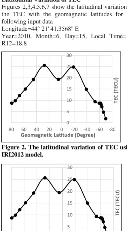
Figures 2,3,4,5,6,7 show the latitudinal variation of the TEC with the geomagnetic latitudes for the following input data

Longitude=44° 21' 41.3568'' E

Year=2010, Month=6, Day=15, Local Time=12, R12=18.8

Figure 2. The latitudinal variation of TEC using IRI2012 model.

Figure 3. The latitudinal variation of TEC using Simpson method.

Figure 4. The latitudinal variation of TEC using Trapezoidal method.

Figure 5. The latitudinal variation of TEC using NeQuick2 model.

Figure 6. The latitudinal variation of TEC using Simpson method.

Figure 7. The latitudinal variation of TEC using Trapezoidal method

The mean absolute percentage error (MAPE) which is given by (16):

𝑀𝐴𝑃𝐸 = 100_𝑛 ∑𝑛_𝑖=1|𝑇𝐸𝐶(𝑝𝑟𝑒𝑑𝑖𝑐𝑡𝑒𝑑)−𝑇𝐸𝐶 (𝑒𝑠𝑡𝑖𝑚𝑎𝑡𝑒𝑑)_{𝑇𝐸𝐶(𝑝𝑟𝑒𝑑𝑖𝑐𝑡𝑒𝑑)} | …..5

The MAPE values for both the numerical integration methods compared with both IRI2012 and NeQuick2 models are given in Table 1.

0 5 10 15 20 25 30

-80 -60 -40 -20 0 20 40 60 80

TE

C

(TE

CU)

Geomagnetic Latitude (Degree)

0 5 10 15 20 25 30

-80 -60 -40 -20 0 20 40 60 80

TE

C

(TE

CU)

Geomagnetic Latitude (Degree)

0 5 10 15 20 25 30

-80 -60 -40 -20 0 20 40 60 80

TE

C

(TE

CU)

Geomagnetic Latitude (Degree)

0 5 10 15 20 25

-80 -60 -40 -20 0 20 40 60 80

TE

C

(T

ECU

)

Geomagnetic Latitude (Degree)

0 5 10 15 20 25

-80 -60 -40 -20 0 20 40 60 80

TE

C

(TE

CU)

Geomagnetic Latitude (Degree)

0 5 10 15 20 25

-80 -60 -40 -20 0 20 40 60 80

TEC

(TECU)

Table 1. The MAPE values for the numerical integration methods

IRI2012 NeQuick2

Numerical Method

Simpson Trapezoidal Simpson Trapezoidal

0.0253 0.02273 0.0213 0.0124

From Table 1, it is shown that the results of TEC obtained using the trapezoidal method has good correspondence with the results of TEC obtained using IRI2012 and NeQuick2 models than for Simpson method. Figures (1-6) provides an important up normal (anomaly) phenomena called equatorial ionization anomaly (EIA). In the equatorial low latitudes ionosphere at F region the ionization density distribution is characterized by a trough at the equator and dual crests on other sides of the equator, are called the crests of EIA (17).

Seasonal Variation of TEC

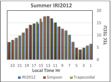
Figures 8, 9, 10, 11 represent the seasonal variation of TEC using

IRI2012 model compared with the results obtained using the numerical integration methods. The study includes two years (March 2010 to February 2011). Each year has three seasons, equinox (March and April, September and October), summer (May, June, July and August) and winter (November and December of current year 2010, January and February of successive year 2011). The following procedure and input data for calculating the TEC.

Input Data

Date: 15th of each month of the year 2010-2011. Location: Baghdad City

Procedure

1. Calculate the hourly variation of TEC using numerical methods.

2. Estimate the average of TEC for each hour of the month of the season.

3. The result of step 2 provides the seasonal mean of the TEC.

4. The comparison of the results of the TEC of step 3 with the TEC obtained from IRI2012 model. 5. The estimation of MAPE for both numerical methods.

Figure 8. The seasonal mean variation of TEC for March and April months.

Figure 9 The seasonal mean variation of TEC for May, June, July and August months

Figure 10. The seasonal mean variation of TEC for September and October months.

0 5 10 15 20

1 3 5 7 9 11 13 15 17 19 21 23

TE

C

TE

CU

Local Time Hr

Summer IRI2012

IRI2012 Simpson Trapezoidal

0 5 10 15 20 25

1 3 5 7 9 11 13 15 17 19 21 23

TE

C

(TE

CU)

Local Time Hr

Spring

Equinox IRI2012

IRI2012 Simpson Trapezoidal

0 5 10 15 20 25

1 3 5 7 9 11 13 15 17 19 21 23

TE

C

(TE

CU)

Local Time Hr

Autumn Equinox IRI2012

Figure 11. The seasonal mean variation of TEC for November, December 2010, and January and February 2011.

Figures 8, 9, 10, 11 present three important facts, first, the local time variation of total electron content (TEC), in general, has a maximum value at daytime hours and decreases at nighttime hours. The maximum value occurs in the local time interval (10-16 hr) for each season approximately. Secondly, the seasonal variation of TEC for spring equinox (March and April months) has the largest value compared with other seasons. Numerically, the values of TEC for spring, summer, autumn and winter seasons equal to 23.317 TECU at 13 hr, 17.896 TECU at 12 hrs, 21.521 TECU at 13 hr and 17.936 TECU at 12 hrs respectively. The largest values were for spring and autumn equinoxes came from the dense ionosphere at these times. Finally, both numerical integratin methods have mean absolute percent error as shown in Tables 2 and 3.

Table 2. The MAPE values for the numerical integration methods for spring and autumn months

Season

Spring Equinox Autumn Equinox

Simpson Trapezoidal Simpson Trapezoidal 0.01093 0.01015 0.008254 0.0066297

Table 3. The MAPE values for the numerical integration methods for summer and winter months.

Season

Summer Winter

Simpson Trapezoidal Simpson Trapezoidal 0.04682 0.04548 0.01253 0.01231

From Tables 2 and 3, it has been noticed that the numerical integration method called trapezoidal method is more accurate than the Simpson method. The smallest MAPE occured for autumn equinoxes with 0.008254 and 0.006629 for

Simpson and Trapezoidal methods respectively, where the largest took place at summer months with 0.046828 and 0.04548 for Simpson and Trapezoidal methods respectively.

From the above results, it is shown that the latitudinal variation of TEC for this study obey to the anomaly called the Equatorial Ionizatuion Anomaly (EIA) which has two crests about the geomagnetic equator. The seasonal variation of TEC provides a large values at spring and autumn equinoxes than for summer and winter seasons. Also, the Trapezoidal method has the best results than for the Simpson method for clculating the TEC for both latitudinal and seasonal variations.

Conflicts of Interest: None.

References:

1. Stamatis S, Thomas D, Konstantinos V. Dimitrios. TEC and foF2 variations: preliminary results. ANNALS OF Geophysics. 2004; 47(4), 1325-1332. 2. Memarzadeh Y. Ionospheric Modeling for Precise

GNSS Applications. PhD thesis, Delft University, Netherlands, 2009; 1-2.

3. Joseph A. GNSS Environmental Sensing, 2nd Ed. Switzerland: Springer International Publishing AG. 2017; 462 p.

4. Jean CU, John BH. Modelling total electron content during geomagnetic storm conditions using empirical orthogonal functions and neural networks. J. Geophys Res Space Phys. 2015; 120: 11,000-11,012.

5. Rajkumar H, Shyamal KC, Bruce TT, Ashish DG, Ezequiel E, Christiano GM, et al. An empirical model of ionospheric total electron content (TEC) near the crest of the equatorial ionization anomaly (EIA). J. Space Weather Spac, 2016; 6 (A29): 1-9. 6. Louis J, Ippolito J. Communications Atmospheric

Effects, Satellite Link Design. USA, John Wiley and Sons. 2008; p 458.

7. Sanjay K, Leong T, Sirajudeen GR, Chong MS, Devendraa S. Validation of the IRI-2012 model with GPS-based ground observation over a low-latitude Singapore station. EPS. 2014; 66 (17): 10.

8. Xueqin H, Bodo WR. Vertical electron content from ionograms in real time. Rad Sci. 2001; 36(2): 335-342.

9. Daniel K, Jaroslav C. Ground-based measurements of ionospheric dynamics. J. Space Weather Spac. 2018; 8(A29): 10.

10. Ashraf F. NeQuick2 model for single-frequency ionospheric delay mitigation. Geomatics. 2016; 10(2): 179-186.

11. The NeQuick2 Model. The Abdus Salam International Centre for Theoretical Physics (ICTP), Italy. 2012; Available at: http://t-ict4d-ictp.it/. 12. Patel NC, Karia SP, Pathak KN. Comparison of

GPS-derived TEC with IRI-2012 and IRI-2007 TEC predictions at Surat, a location around the EIA crest in the Indian sector, during the ascending phase of solar cycle 24. Adv Space Res. 2017; 60: 228-237.

0 5 10 15 20

1 3 5 7 9 11 13 15 17 19 21 23

TE

C

(

TE

CU)

Local Time Hr

Winter IRI2012

13. The International Reference Ionosphere model IRI, 2012. Available at: http://irimodel.org/.

14. Richard LB, Faires JD, Annette, MB. Numerical Analysis, 10th .USA, Boston. Cenveo Publisher services. 2016; p 918.

15. Space Weather Services, Australian Government/

Bureau of Meteorology. 2018; Available at:

www.sws.bom.gov.au/.

16. Chris T. A better measure of relative prediction accuracy for model selection and model estimation. J. Oper Res Soci. 2015; 66: 1352-1362.

17. Nilesh CP, Sheetal PK, Kamlesh NP. GPS-TEC Variation during Low to High Solar Activity Period (2010-2014) under the Northern Crest of Indian Equatorial Ionization Anomaly Region. Positioning. 2017; 8: 13-35.

ةيددعلا قرطلا مادختساب ةفلتخم لوصف و ضرع رئاود قوف يلكلا ينورتكللاا ىوتحملا ليلحت و باسح

همعن نيسح يلع

قارعلا ,دادغب ,ةيرصنتسملا هعماجلا ,مولعلا ةيلك ,وجلا مولع مسق

:ةصلاخلا

TEC .ةيفارغجلا ةحلاملا ماظنل مهم لماع وه ريفسونويلال

باسح مت ةساردلا هذه يف TEC

مهاسم امدختسم ,قارعلا ,دادغب ةنيدم قوف هبش ةقيرط و ةبكرملا نوسبمس ةقيرط امه نييددع نيتقيرط ة

.ةبكرملا فرحنملا TEC

يجذومنإ ةطساوب ةلصحتسملا ةينورتكللاا ةفاثكلل يطخلا لماكتلا مادختساب بسح IRI2012

و NeQuick2 نم

عافترا 70 ىلا 2000 Km و ةنسلا نم مويلا و مويلا نم هعاسلا .ضرلاا حطس قوف R12

ك تريتخا رظنب نيذخا باسحلا قرطل تلاخدم

ل ةيلصفلا و ةيمويلا و ةيفارغجلا تاربغتلا رابتعلاا TEC

ريغت جئاتن . TEC

و يئاوتسلاا نيأتلا ذوذشب ىمسي ذوذش تنيب ضرعلا طوطخ عم

ل نيتمق هيف رهظي يذلا TEC

قلطملا اطخلا ةبسن لدعم .يسيطانغمويجلا ءاوتسلاا لوح MAPE

ليلحتلا قرط نم ةلصحتسملا جئاتنلل

يلاتلاك تناك هلاعا نيجذومنلا امدختسم يددعلا 0.0253

و 0.02273 ,

0.0213 و

0.0124 دقف يلصفلا ريغتلا جئاتن اما .يلاوتلا ىلع

ميق نا تحضوا TEC

ميق تغلب .ةيوتشلا و ةيفيصلا ميقلا نم ربكا يفيرخلا و يعيبرلا نيلادتعلال MAPE

رلل عيب 0.01093 و

0.01015

تغلب دقف ءاتشلا و فيصلا و فيرخلا لوصفل اما .يلاوتلا ىلع فرحنملا هبشو نوسبمس يتقيرطل 0.005825

و 0.006629 ,

0.04682 و

0.0454 , 0.01253 و

0.01231 .يلاوتلا ىلع فرحنملا هبشو نوسبمس يتقيرطل

ةيحاتفملا تاملكلا :

,ةينورتكللاا ةفاثكلا GNSS

, جذومنأ ,ريفسونويلاا ,يملاعلا ديدحتلا ماظن IRI2012