* Corresponding author
E-mail: [email protected] (A. Costa) © 2018 Growing Science Ltd. All rights reserved. doi: 10.5267/j.ijiec.2017.8.003
International Journal of Industrial Engineering Computations 9 (2018) 331–348
Contents lists available at GrowingScience
International Journal of Industrial Engineering Computations
homepage: www.GrowingScience.com/ijiecSingle machine batch processing problem with release dates to minimize total
completion time
Pedram Beldara and Antonio Costab*
aDepartment of Industrial and Mechanical Engineering, Qazvin Branch, Islamic Azad University, Qazvin, Iran bUniversity of Catania, DICAR, Viale Andrea Doria 6, 95125 Catania, Italy
C H R O N I C L E A B S T R A C T
Article history: Received July 18 2017 Received in Revised Format July 29 2017
Accepted August 19 2017 Available online August 20 2017
A single machine batch processing problem with release dates to minimize the total completion time (1|rj,batch|
Cj) is investigated in this research. An original mixed integer linearprogramming (MILP) model is proposed to optimally solve the problem. Since the research problem at hand is shown to be NP-hard, several different meta-heuristic algorithms based on tabu search (TS) and particle swarm optimization (PSO) are used to solve the problem. To find the most performing heuristic optimization technique, a set of test cases ranging in size (small, medium, and large) are randomly generated and solved by the proposed meta-heuristic algorithms. An extended comparison analysis is carried out and the outperformance of a hybrid meta-heuristic technique properly combining PSO and genetic algorithm (PSO-GA) is statistically demonstrated.
© 2018 Growing Science Ltd. All rights reserved
Keywords:
Minimization of total completion time
Batch processing Single machine scheduling Mathematical programming Scheduling with release dates
1. Introduction
Batch processing (BP) problem has been attracting many academics and practitioners because of its intensive applications in the real-world industry. In BP, a resource is able to process more than one job as a batch at the same time. BP problems can be observed in different industries such as cutting machines in textile industry, testers in semiconductors manufacturing, and ovens in metalworking. A similar problem wherein jobs must be grouped into batches and contemporarily sequences of jobs and batches must be managed to satisfy a certain objective is also ascribable to the fields denoted as scheduling with tool changes (Costa et al., 2016) and group scheduling (Costa et al., 2017).
each batch based on one of the jobs attributes such as weight or volume; c) the jobs assigned to a batch must respect both conditions explained in (a) and (b).
Most of the research performed in BP problems have been focused on category (2) as for processing time of each batch and categories (a) or (b) as for the capacities of the batches. Chandru et al. (1993) propose an exact procedure and several heuristics for solving the 1|batch|
Cjproblem for categories (2) and (a). Uzsoy (1994) tackles both 1|batch|Cmax and 1|batch|
Cjproblems and proposes an exact procedure based on Branch and Bound (B&B) algorithm for the 1|batch|
Cjproblem. Moreover, he devises several heuristics to solve those problems for categories (2) and (b) and proves that both problems are NP-hard. Another research of Uzsoy and Yang (1997) deals with the 1|batch|
w Cj jproblem for categories (2) and (a). They propose several heuristics and an exact approach based on B&B algorithm. Jolai and Dupont (1997) approach the 1|rj,batch|Cmax problem for categories (2) and (b) and propose anumber of heuristics for the problem. Lee (1999) studies the 1|rj,batch|Cmax problem for categories (2)
and (a). He proposes several polynomial and pseudo-polynomial time algorithms for a few particular instances and develop efficient heuristics for the general problem. Liu and Yu (2000) approach the 1|rj,batch|Cmax problem for categories (2) and (a) and propose a pseudo-polynomial algorithm for the
case with a constant number of release dates and a greedy heuristic for the general case. Dupont and Dhaenens-Flipo (2002) address the 1|rj,batch|Cmax problem for categories (2) and (b) and develop an
exact procedure based on B&B method for the research problem. Chang and Wang (2004) develop a heuristic algorithm for the 1|rj, batch|
Cj problem for categories (2) and (b). Melouk et al. (2004) andDamodaran et al. (2006) develop several meta-heuristic algorithms based on simulated annealing (SA) and genetic algorithm (GA) for the 1|batch|Cmax problem for categories (2) and (b). Damodaran et al.
(2007) cope with the 1|batch|Cmax problem for categories (2) and (c) and develop a meta-heuristic
algorithm based on SA to solve the problem. Parsa et al. (2010) approach the 1|batch|Cmax problem for
categories (2) and (b) and propose an exact approach based on Branch and Price (B&P) algorithm. They compare their proposed algorithm with the B&B method proposed by Dupont and Dhaenens-Flipo (2002) and show that the B&P algorithm is better than the B&B algorithm. Xu et al. (2012) solve the 1|rj,batch|Cmax problem for categories (2) and (b) through a mixed integer linear programming (MILP)
model. They develop an effective lower bound method, a heuristic algorithm, and an ant colony optimization (ACO) algorithm for solving the mentioned BP problem. Lee and Lee (2013) develop several heuristics for the 1|batch|Cmax problem for categories (2) and (b). Jia and Leung (2014) provide
an improved max-min ant system algorithm for the 1|batch|Cmax problem for categories (2) and (b). Zhou
et al. (2014) approach the 1|rj,batch|Cmax problem for categories (2) and (b) and propose various heuristics
to solve the problem. Al-Salamah (2015) devises an artificial bee colony method to minimize the 1|batch|Cmax problem for categories (2) and (b). Li et al. (2015) consider the 1|batch, dj=d|
(EjTj) problem for categories (2) and (b) and develop a hybrid GA by combining GA with a heuristic algorithm managing the batches. Parsa et al. (2016) introduce a hybrid meta-heuristic algorithm based on the max-min ant system for 1|batch|
Cjfor categories for (2) and (b).P. Beldar and A. Costa
onto boards and then, the boards are put into an oven. The number of boards that can process at the same time is described as oven capacity. Thus, the boards must be split into batches. The processing time of a batch is defined by the longest processing time among all jobs in that batch. The processing time in burn-in operations is too lengthy compared to other testburn-ing operations. Thus, they form a bottleneck burn-in the final stage. The minimization of the total completion time would ensure the increase of the throughput. In this research, it is assumed that n jobs are assigned to a machine to be processed. The machine can process the jobs arranged into batches. All jobs are not available at the beginning of the planning horizon. The machine has a size capacity and also can process at most a limited amount of jobs at the same time. Each job has a different size. The processing time of each batch is equal to the maximum processing time of jobs assigned to the batch. The goal is to minimize the total completion time of jobs.
The rest of this paper is organized as follows. In Section 2 a mathematical model is developed for the proposed research problem. In Section 3 several meta-heuristic algorithms are proposed to heuristically solve the problem. The specifications of the test problems used to compare the performance of the proposed algorithms, also including parameter settings and solution time are explained in Section 4. In Section 5 numerical results and comparison analysis involving the proposed metaheuristic algorithms are presented. In Section 6 conclusions and future research areas are discussed.
2. The Mathematical Model
In this section, an original MILP model is developed for the proposed research problem. In this model, a batch is considered to be active whether it has at least one job and the maximum number of batches is equal to the number of jobs. Indexes, parameters, decision variables, and the whole mathematical model are as follows:
Indexes:
j Index of jobs
b Index of batches
Parameters:
n The number of jobs
B Capacity of machine
N The maximum number of jobs can be assigned to a batch
M A large number
pj The processing time of job j, j=1,2,…,n
rj The release date of job j, j=1,2,…,n
sj The size of job j, j=1,2,…,n
Decision variables:
1 if job is assigned to batch
1,2,..., & 1,2,..., 0 otherwise
jb
j b
X j n b n
1 if batch is active
1,2,..., 0 otherwise
b
b
y b n
The model
1 min n j
j C
(1) subject to 11 1, 2, ...,
n
jb b
X j n
(2)1
1, 2, ..., n
jb j b j
X s By b n
(3)1
1, 2, ..., n
jb j
X N b n
(4)1, 2, ..., ; 1, 2, . ..,
b
jb j
P X p j n b n (5)
1, 2, ..., ; 1, 2, . ..,
b jb j
S X r j n b n (6)
1 1
2, 3, ...,
b b b
S S P b n (7)
1
1, 2, ..., ; 1, 2, ..., b bj jb
C S P X M j n b n (8)
1
1, 2, ..., n
jb b j
X y b n
(9)1 1, 2, ..., 1
b b
y y b n (10)
0,1jb
X , Yb
0,1 , Cj0 ...,j 1, 2, ..., ; n b1, 2, n (11) The objective, as presented by Eq. (1), is to minimize the total completion time. Constraint (2) is incorporated into the model to ensure that each job is assigned to one batch. Constraint (3) guarantees that the total size of the jobs assigned to a batch does not exceed the batch capacity. Constraint (4) assures that the number of jobs assigned to a batch cannot be greater than the number of jobs to be assigned to each batch. Constraint (5) allows the processing time of each batch is equal to or greater than the processing time of the jobs assigned to that batch. Constraint (6) ensures that the starting processing time of a batch is greater than or equal to the arrival time of all jobs assigned to that batch. According to Constraint (7) the single-machine cannot process more than one batch at a time. Constraint (8) states the completion time of a job is equal to the completion time of the batch the job is assigned to. Constraint (9) ensures at least one job is allocated to an active batch. Constraint (10) guarantees that all active batches are ordered consecutively.Since Uzsoy (1994) proved that the 1|batch|
Cj problem for categories (2) and (b) is an NP-hard problem, the single machine batch processing problem under investigation, with release dates to minimize of the total completion time (1|rj,batch|
Cj) for categories (2) and (c), can be classified as an NP-hard problem too. As a result, meta-heuristic algorithms are needed to solve large-sized issues.3. Meta-heuristic algorithms
P. Beldar and A. Costa
algorithms try to make an improvement on multiple candidate solutions at each iteration. Genetic Algorithms (GAs), Ant Colony Optimization (ACO), particle swarm intelligence (PSO) fall under this class. In this research, due to the significant performance of TS and PSO in solving relevant BP scheduling problems (Liao and Huang (2011), Damodaran et al. (2012) and Damodaran et al. (2013)), both of them have been taken into account for solving the research problem under investigation. The following sections deal with the adopted algorithms in depth.
3.1 Tabu Search
Tabu Search (TS) was originally developed by Glover and Laguna (1999) and basically consists of a neighborhood search method that keeps track of the up-to-now search path to avoid to be trapped into local optima or to try an explorative search of the solution domain (Costa et al., 2015). The proposed TS was inspired to that of Liao and Huang (2011) but, differently from the original one, in this paper an enhanced two-level TS algorithm was devised. In the first level (inside level), the best assignment of jobs to batches is examined. In the second level (outside level), the best sequence of batches is investigated. The relationship between the aforementioned phases is that once the inside level search is carried out to assign jobs to batches, the search process is switched to the outside level. In fact, whenever the inside level search stopping criterion is met, the best obtained job assignment is considered and the search strategy changes to the outside level. The outside search stops when the related stopping criterion is met. The best obtained solution, which combines a sequence of batches and the allocation of jobs to each batch, is the final solution. The peculiarities of the proposed TS are as follows.
3.1.1 Initial Feasible Solution
In this research, an effective procedure inspired to the heuristic algorithm called DYNA (Jolai & Dupont, 1997) is proposed to generate the initial feasible solution to be handled by the inside level. Then, the best solution obtained by the inside level becomes the initial feasible solution for the subsequent phase, i.e., the outside level. The algorithm generating the initial solution works as follows:
Step 1: First, the jobs are ordered based on the Earliest Completion Time (ECT) sorting rule. In words, jobs are ordered in nondecreasing order of their expected completion time (rj + pj), with ties broken by rj.
Step 2: The first job in the ECT list is assigned to the first batch.
Step 3: The subsequent job is scheduled according to the following criteria:
Step 3.1: The job on the top of the list of remaining jobs is assigned separately to the existing batches having enough space.
Step 3.2: If the job on the top of the list of remaining jobs cannot be allocated to any batch, a new batch is created and the job is assigned to it.
Step 4: Then the total completion time is calculated for all possible combinations.
Step 5: The state with the minimum total completion time among all possible states is selected. Step 6: All jobs have been scheduled. Go to Step7. Otherwise go to Step3.
Step 7: Stop algorithm.
3.1.2 Neighborhood generation mechanism
After an initial feasible solution is generated, the neighborhood search at the inside level is performed by two moves, the former being a swap move and the latter being an insert move:
Swap move. The job in ath position of bth batch is swapped with the job in kth position of gth batch. if bth and gth batches have enough space the move is feasible. Otherwise the move is unfeasible and it is rejected from the neighborhood.
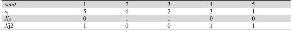
Let us consider a BP problem with n=5 jobs and two batches. The maximum number of items per batch is N=3 and B=10 is the machine capacity. The seed solution is [1-2-3-4-5] while the size of each job sj as
well as the batch i each job is allocated to, i.e., Xji, are reported in Table 1. Six distinct moves are allowed
by applying the swap operator as follows: (2,1), (2,4), (2,5), (3,1), (3,2), (3,5). Move (3,1) is not feasible as the obtained batch size (6+5) exceeds the provided maximum capacity B=10. As far as the insertion operator is concerned, since N=3, the following three different moves may be generated: (2,3,1), (2,3,4), (2,3,5). Only the last move is feasible under the batch size viewpoint. As a result, just six out of nine moves can be considered as candidates to be the next seed.
Table 1
An example of seed solution
seed 1 2 3 4 5
sj 5 6 2 3 1
Xj1 0 1 1 0 0
Xj2 1 0 0 1 1
As for as the outside level, the neighborhood is generated according to a regular adjacent pairwise interchange method; thus, β-1 alternative moves may be produced, where β is the current amount of batches. Hence, β-1 additional moves have to be considered for selecting the next seed solution.
3.1.3 The Tabu List (TL)
TL is a list of the characteristics of forbidden moves. It prevents the cycling back to formerly visited solutions by storing the characteristics of these moves for a certain period. At each iteration, the best neighbor solution, i.e., that one with the best objective function value, is selected and the move that generated that candidate solution is compared with the moves stored in the TL. Whether the move does not exist in the TL, the corresponding solution is selected as a new seed solution that, subsequently, will be subject again to the neighborhood generation mechanism. Otherwise, the move associated to the next best solution is taken into account. If a tabu move allows a better objective function value than the best global one found so far, the tabu restriction is ignored and the solution related to that move is selected as the new seed solution. The best objective function value found so far is denoted as the aspiration criterion.
3.1.4 Stopping Criterion
The aforementioned process is repeated until the stopping criterion based on the maximum time designated for each problem is met.
3.2 The PSO
The PSO algorithm, introduced by Kennedy and Eberhart (1995), is a population-based algorithm to solve continuous optimization problems. It starts with a set of initial solutions (particles). Each particle has its own position and velocity vector. The position vector 1, 2,...,
t t t t
i i i in
X x x x represents the position of the ith particle in the tth iteration where t
ij
x illustrates the jth dimension of the n-dimensional position vector. The velocity vector 1, 2,...,
t t t t
i i i in
V v v v represents the velocity of the ith particle in the tth iteration where t
ij
v illustrates the jth dimension of the n-dimensional velocity vector. The dimension of search space is equal to the number of jobs n in this research. The successful behavior of each particle affects the behavior of other particles, so particles move toward areas with better objective function values according to the two following targets:
Pbest: The best position visited by the ith particle at the tth iteration is shown as Pbest,
1, 2,...,
t t t t
i i i in
P. Beldar and A. Costa
Gbest: The best position visited by all particles at the tth iteration is called Gbest,
1, 2,...,
t t t t
i Gbest Gbe n
Gbest Gbest st .
Since particles move towards better positions during the search process, the velocity of each particle changes on the basis of Pbest and Gbest vectors at each iteration. The velocity of each particle at each iteration is updated by:
1
1 1 2 2 ,
t t t t t t
i i i i i
V wV c r Pbest X c r Gbest X (11)
where w is the inertia weight which controls the impact of the previous velocity vector at the tth iteration while c1 and c2 are two constants called acceleration coefficients. Also, r1 and r2 are random numbers
drawn from a uniform distribution U[0, 1]. The position of each particle varies as velocity changes. As a result, the position of the ith particle at the (t + 1)th iteration is updated as follows:
1 1
t t t
i i i
X X V (12)
3.2.1 PSO encoding
The original PSO algorithm is used to solve the continuous optimization problems. Arabameri and Salmasi (2013), and Tadayon and Salmasi (2013) apply the smallest position value (SPV) rule that is an increasing order mechanism to transform a continuous PSO to a discrete one. In other words, the SPV method allows transforming a real-encoded solution into a permutation one, that is a sequence of jobs. For instance, assume that t
i
X =[2.3,-1.5,-2.03,1.16] is the position vector of the ith particle at the tth iteration whose dimension is equal to four (i.e., four jobs). Since -2.03 is the smallest value in t
i X , the third member of the position vector, that is J3, is located in the first position of the sequence. The second
smallest value is -1.5, so J2 will be the second digit of the sequence, and so on. Following the same
fashion, the final permutation sequence will be: J3-J2-J4-J1.
3.2.2 Initial solutions
In this research, three members (particles) of the initial population are created by the following dispatching rules: shortest processing time (SPT) (Baker & Trietsch, 2009), earliest release date (ERD) (Baker and Trietsch, 2009), and ECT. The rest of the members are randomly generated.
3.2.3 Updating Particles
Based on Poli et al. (2007), if a multiplier χ is inserted into Eq. (11), the convergence speed as well as the effectiveness of PSO algorithm may be improved. The appropriate value of χ is calculated through the following Equations:
1 2
, c c 4
(13)
22
2 4
(14)
To satisfy Eq. (13), the value of 2.05 is considered for both c1 and c2. Therefore, according to Eq. (14),
is equal to 7298. As a result, the new expression for the velocity vector of each particle is:
1
1 1 2 2
t t t t t t
i i i i i
V wV c r Pbest X c r Gbest X
(15)
3.2.4 Improving the performance of PSO
Pros and cons characterize the particle swarm optimization algorithm (Coello Coello et al., 2007). The main advantage of PSO consists of its ability in exploitation while it may give weak result in exploring the solution space. In order to boost the performance of PSO, a series of hybrid PSO algorithms, which combine PSO with other performing search techniques, have been developed by literature so far (Sha & Hsu, 2006; Xia & Wu, 2006; Chen et al., 2013; Gao et al., 2014; Javidrad & Nazari, 2017).
Notably, Arabameri and Salmasi (2013) demonstrated as the performance of PSO may be significantly improved if it is combined with a proper neighborhood search. In this research, two different hybrid methods have been considered to boost the performance of the regular PSO, the former being based on GA (PSO-GA), the latter being focused on TS (PSO-TS).
PSO-GA. The GA, just like the PSO, is a population-based stochastic algorithm that evolves through a number of initial solutions called chromosomes. At each iteration, a series of basic operators called selection, crossover and mutation are performed on the population with the aim of performing both exploration and exploitation (Michalewicz, 1996; Lin & Kang, 1999). In this research, the selection of offspring is randomly executed on the population in order to strengthen the diversification phase. An arithmetic crossover operator based on Simon (2013) was employed to produce two chromosomes called offspring by combining two parent chromosomes. In this method, the genes related to two randomly selected individuals (ith and jth particles) are exchanged and modified through Eq. (16) and Eq. (17), where αl is an l-dimensional vector of random weights between 0 and 1. X1kl and X2klrepresent the offspring particles at the kth iteration. The part of population on which the crossover operator is executed at each iteration depends on the crossover rate pc.
1kl l il 1 l jl 1, 2, ,
X
X
X l n (16)
2kl l jl 1 l il 1, 2, ,
X
X
X l n (17)The goal of mutation is to maintain the population diversity, thus avoiding any premature convergence. It makes a new offspring up from a single parent and assists the algorithm to avoid to be trapped in local optima. A single parent (ith particle) is selected randomly to perform a Gaussian mutation procedure based on Simon (2013). Then, the jth element of the selected particle (Xi) is varied according to Kuo and
Han (2011), as follows:
0,1 [0,1]new ij ij
X X N rand (18)
where N(0,1) is a number from a standard normal distribution and rand[0,1] is a random number form a uniform distribution in the range [0,1]. The portion of population in which mutation procedure is applied to depends on the mutation rate (pc). A pseudo-code of the proposed PSO-GA is reported in the following
paragraph.
Pseudo-code of PSO-GA
Step 1. Initialize control parameters and create a swarm with P particles. Do While (stopping criterion is not met)
Step 2. Update position and velocity vectors fori= 1 to P
forj=1 to n
1
1 1 2 2
t t t t t t
i i i i i
V wV c r Pbest X c r Gbest X
end for end for
Step 3. Arithmetic crossover operator fork=1 to nc
P. Beldar and A. Costa
forl=1 to n
X1kl lXil
1 l
Xjl X2kllXjl
1 l
Xilend for end for
Step 4. Gaussian mutation operator forq=1 to nm
Select one single parent randomly (ith) and change the jth element of it
new
0,1 [0,1]ij ij
X X N rand
end for
Step 5. New particles
Merge all the newly generated particles yielded by the crossover, the mutation, and PSO operators. Then, select the best P particles in terms of objective function value.
Step 6. Update the Pbestand Gbestvectors fors=1 to P
if (f(Xs) < f(Pbests))
Pbests= Xs end if if (f(Pbests) < f(Gbest))
Gbest = Pbests end if
end for
update inertia weight loop
PSO-TS. Actually, three different versions of PSO-TS, hereinafter denoted with the subscripts a, b and c, have been developed as explained below:
a) In the first version, whenever the Gbest is updated at a certain iteration, it is given to TS as a seed solution and TS is performed for a finite amount of time. If a better solution is found, it is considered as the new Gbest.
b) In this version, whenever the Pbest is updated at a certain iteration, it is given to TS as a seed solution and TS is performed for a finite amount of time. If a better solution is found, it is considered as the new Pbest.
c) In the last scenario, PSO and TS are hierarchically applied to the problem at hand. The regular PSO is executed in the first phase until a switching criterion is satisfied. Subsequently, the best solution found by the PSO is handled by the TS algorithm until a time-based stopping criterion is met.
It is worthy to point out that the aforementioned versions of hybrid PSO are powered by the same two-levels tabu search described in Section 3.1.
3.2.5 Calculating the objective function
Based on empirical studies, an appropriate assignment of jobs to the batches has a considerable effect on the value of the objective function. Therefore, the proposed heuristic algorithm as in Section 3.1.1 was employed to calculate the total completion time of each solution.
4. Computational experiments
4.1 Test problems
To evaluate the performance of the proposed algorithms, a wide range of test problems has randomly been generated on the basis of the following five different factors: the number of jobs (n), the maximum number of jobs in a batch (N), the maximum capacity of the machine (B), the size of jobs (sj) and the
processing time of jobs (pj). Three different classes of problems (small, medium, large) have been
provided for each factor, as depicted in Table 2. Hence, the total amount of scenario problems to be investigated is 35 = 243.
Table 2
Settings about the test problems
Factor/Class Small Medium Large
n U[5, 20] U[21, 50] U[51, 100]
N 3 5 7
B 10 15 20
sj U[1, 5] U[1, 10] U[4, 10]
pj U[1, 10] U[1, 20] U[1, 50]
Two replicates have been considered for each class; thus, a total amount of 486 test problems have been solved by means of each algorithm. As far as the release dates are concerned, they are drawn from the uniform discrete distribution U[0,( / ) max( )j
j
n N p ] and then rounded to the closer integer value; max(pj)
is the maximum value of processing time among the n jobs.
4.2 Setting of control parameters
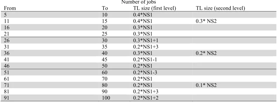
Both effectiveness and efficiency of metaheuristic algorithms can be enhanced by giving appropriate values to their control parameters. As for TS algorithm the most influencing parameter to be chosen is the TL size. In this paper an empirical formula for choosing the TL size has been conceived making use of a trial-and-error approach involving an extended number of instances. Table 3 shows how the TL size should be set for both the first and the second level, on the basis of the expected neighborhood size.
Table 3
The different values of TL size for different number of jobs
Number of jobs
From To TL size (first level) TL size (second level)
5 10 0.4*NS1
11 15 0.4*NS1 0.3* NS2
16 20 0.3*NS1
21 25 0.3*NS1
26 30 0.3*NS1+1
31 35 0.2*NS1+3
36 40 0.3*NS1 0.2* NS2
41 45 0.2*NS1-1
46 50 0.2*NS1
51 60 0.2*NS1-3
61 70 0.2*NS1
71 80 0.2*NS1 0.1* NS2
81 90 0.2*NS1+3
91 100 0.2*NS1+2
In fact, especially for the first level of TS, the neighborhood size (NS1) is not a priori known as it depends on how the jobs are allocated to the batches, conforming to the other parameters, i.e., N, B, sj. On the
P. Beldar and A. Costa
the current number of batches. To calculate both NS1 and NS2 the heuristic described in Section 3.3.1 has been employed. Whether the TL size in Table 3 does not yield any integer number, the obtained result must be properly rounded down. The control parameters pertaining to the other proposed algorithms (i.e., PSOa, PSOb, PSOc, PSO-GA) have been tuned through the response surface methodology (RSM) method. RSM is a collection of statistical and mathematical techniques used for developing, improving, and optimizing processes. In RSM, there are various input variables (control parameters) that can potentially influence some performance measures or quality characteristics that are called response (the objective function of the algorithm). Usually, in the RSM approach, it is convenient to transform the original variables into coded variables x1,x2,...,xl, which are usually defined to be dimensionless with mean zero and the same spread or standard deviation (Raymond et al., 2009). Eq. (190 shows how to transform an original variable to a coded one, where Xi and xi represent the actual
variable and the coded variable, respectively. Thus, the response function can be written as in Eq. (20).
2
2
High Low i
i
High Low
X X
X x
X X
,
(19)
1, , , 2 l
y x x x , (20)
where l represents the number of input variables. The goal is to gain the most suitable level of the algorithm parameters to optimize the response value. The main hypothesis is that the independent variables are continuous and controllable by experiments with negligible errors. Finding a proper approximation for the true functional relationship between independent variables and the response surface is required (Kwak, 2005). Raymond et al. (2009) proposed a second-order model, as follows:
2 0
1 1
l l l
j j jj j ij i j
j j i j
y x x x x
(21)where y is the predicted response, β0 is the model constant, βj is the linear coefficient, βjj is the quadratic
coefficient, and βij is the interaction coefficient.
Shi and Eberhart (1999) stated that a large value of inertia weight w simplifies probing new positions (global search), while a small value of inertia weight simplifies a local search. As a result, a suitable balancing between local and global search can be achieved by adaptively reducing the inertia weight linearly according to Eq. (22), where t indicates the time of the current iteration and T refers to the total time considered for each test problem, respectively. Also, wstart and wend are the starting and the finishing
values for the inertia weight, respectively.
start start end t
w w w w
T
(22)
Basically, NP, wstart, and wend, pc, and pm are the control parameters considered as the input variables for
PSO-GA. The input variables of the other PSO-based algorithms (namely PSOa, PSOb, and PSOc) are NP, wstart, wend and TL size. According to Eq. (19), the PSO-GA parameters are denoted by X1(NP), X2(wstart), X3(wend), X4(pc), X5(pm), while the other control parameters are denoted by X1(NP), X2(wstart), X3(wend), X4(TL size). Each control parameter has been varied at three levels, conforming to low (-1),
center (0) and high level (+1), as depicted in Table 4 and Table 5. As concerns the NP parameter, three scenarios depending on the problem size have been taken into account. The Box-Behnken experimental design was employed to handle a family of efficient three-level designs fitting the second-order response surfaces (Raymond et al., 2009). The number of experiments is equal to 2l(l-1)+nc, where nc is the number
Table 4
The levels of the values of each parameter for PSO-GA
Parameter/Level Low (-1) Center (0) High (+1)
NP (small size) 10 20 30
NP (medium size) 40 50 60
NP (large size) 70 80 90
0.1 0.3 0.5
0.7 0.9 1.1
0.7 0.8 0.9
0.1 0.2 0.3
Table 5
The levels of the values of each parameter for PSO , PSO , and PSO
Parameter/Level Low (-1) Center (0) High (+1)
NP (small size) 10 20 30
NP (medium size) 40 50 60
NP (large size) 70 80 90
0.2 0.4 0.6
0.9 1.1 1.3
0.1*NS 0.25* NS 0.4* NS
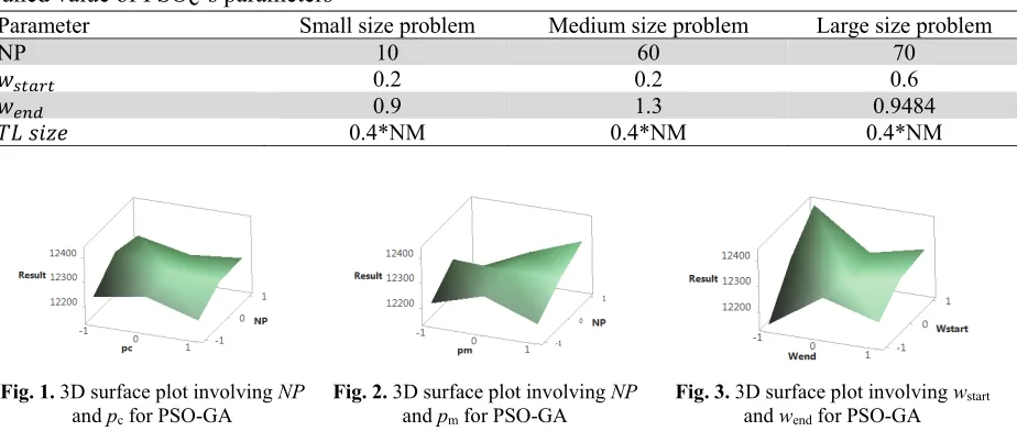
Tables 6, 7, 8, and 9 show the optimal values of control parameters obtained by means of the RSM-based calibration. Due to representation purposes, Figs. (1-3) illustrate the 3D surface plots involving the different PSO-GA control parameters.
Table 6
Tuned value of PSO-GA’s parameters
Parameter Small size problem Medium size problem Large size problem
NP 10 40 70
0.5 0.5 0.1
1.1 0.7 0.7
0.7 0.9 0.9
0.3 0.3 0.3
Table 7
Tuned value of PSOa’s parameters
Parameter Small size problem Medium size problem Large size problem
NP 30 40 70
0.2 0.3535 0.6
1.3 0.9 0.9808
0.4*NS 0.1*NS 0.4*NS
Table 8
Tuned value of PSOb’s parameters
Parameter Small size problem Medium size problem Large size problem
NP 10 60 70
0.2 0.2 0.6
0.9 1.3 1.3
P. Beldar and A. Costa
Table 9
Tuned value of PSOc’s parameters
Parameter Small size problem Medium size problem Large size problem
NP 10 60 70
0.2 0.2 0.6
0.9 1.3 0.9484
0.4*NM 0.4*NM 0.4*NM
Fig. 1. 3D surface plot involving NP
and pc for PSO-GA
Fig. 2. 3D surface plot involving NP
and pm for PSO-GA
Fig. 3. 3D surface plot involving wstart
and wend for PSO-GA
4.3. Computational time
The exit criterion of the proposed metaheuristic algorithms is based on the computational time (CT) and, conforming to Gohari and Salmasi (2015), it has been parametrized as a function of the number of jobs (n), as follows:
, max up CT
CT n
n
(23)
where CTmax and nup respectively are the maximum allowed computational time and the upper value of
the range related to the number of jobs; as for example, in the range [5, 20], nup is equal to 20. CTmax has
been set to 30, 90, and 180 seconds for small-, medium-, and large-sized problems, respectively. Hence, the values of δ for small-, medium-, and large-sized problems are equal to 1.5, 1.8 and 1.8, respectively. All the proposed algorithms were coded in C++ programming language. The whole set of experiments was performed on a PC with 2.8 GHz CPU and 2 GB RAM.
5. Numerical results and comparison analysis
In order to compare the different metaheuristics, a Relative Percentage Deviation (RPD) performance indicator as in Eq. (24) has been taken into account. It is worth pointing out that, for most small-size problems, the RPDs have been computed on the basis of the global optima obtained by solving the mathematical problem. Whereas, for both medium and larger-sized issues, each RPD was computed by exploiting the relative local optimum value among the different competing algorithms.
100 algorithm solution optimal solution
RPD
optimal solution
(24)
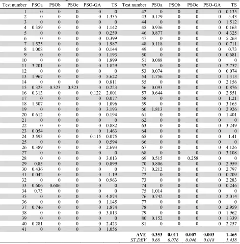
Table 10
Small-sized problems: average RPD results over the two replicates
Test number PSOa PSOb PSOc PSO-GA TS Test number PSOa PSOb PSOc PSO-GA TS
1 0 0 0 0 0 42 0 0 0 0 0.135
2 0 0 0 0 1.335 43 0.179 0 0 0 5.43
3 0 0 0 0 0 44 0 0 0 0 1.512
4 0.359 0 0 0 1.142 45 0.936 0 0 0 0.163
5 0 0 0 0 0.259 46 0.877 0 0 0 4.325
6 0 0 0 0 0.399 47 0 0 0 0 5.263
7 1.525 0 0 0 1.987 48 0.118 0 0 0 0.711
8 1.008 0 0 0 0.144 49 0 0 0 0 0.73
9 0 0 0 0 1.193 50 0 0 0 0 0.681
10 0 0 0 0 1.899 51 0.088 0 0 0 0
11 3.201 0 0 0 1.829 52 0 0 0 0 2.757
12 0 0 0 0 0 53 0.074 0 0 0 0.074
13 1.967 0 0 0 5.622 54 1.756 0 0 0 1.313
14 0 0 0 0 0.811 55 0 0 0 0 2.156
15 0.323 0.323 0.323 0 0.223 56 0.093 0 0 0 0.876
16 0.313 0 0 0.122 2.001 57 0.644 0 0 0 2.551
17 0 0 0 0 0.077 58 0 0 0 0 1.21
18 1.507 0 0 0 1.096 59 0 0 0 0 3.165
19 0 0 0 0 3.193 60 1.813 0 0 0 2.926
20 0.612 0 0 0 0.194 61 0 0 0 0 1.401
21 0 0 0 0 0 62 0 0 0 0 0
22 0 0 0 0 0.882 63 0 0 0 0 3.249
23 0.054 0 0 0 1.463 64 0 0 0 0 0
24 3.593 0 0 0.115 0.075 65 0 0 0 0 1.41
25 0 0 0 0 0.594 66 0 0 0 0 0
26 0.389 0 0 0 2.693 67 0 0 0 0 4.126
27 0 0 0 0 0 68 0 0 0 0 3.108
28 0 0 0 0 3.013 69 0.515 0 0.258 0 0
29 0.85 0 0 0 0.899 70 0.806 0 0 0 2.959
30 0.436 0 0 0 0 71 0.212 0 0 0 2.797
31 0.042 0 0 0 1.19 72 0 0 0 0 0.209
32 0 0 0 0 0.963 73 0 0 0 0 2.283
33 0.606 0.606 0 0 0 74 0 0 0 0 0.246
34 0.73 0 0 0 0 75 1.014 0 0 0 0
35 0 0 0 0 4.874 76 0.742 0 0 0 2.014
36 0 0 0 0 1.145 77 0 0 0 0 0
37 0.746 0 0 0 1.874 78 0 0 0 0 2.959
38 0 0 0 0 3.813 79 0 0 0 0 1.962
39 0 0 0 0 0 80 0.152 0 0 0 1.339
40 0.281 0 0 0 2.423 81 0 0 0 0 2.257
41 0 0 0 0 1.056
AVE 0.353 0.011 0.007 0.003 1.465
ST.DEV 0.68 0.076 0.046 0.018 1.458
P. Beldar and A. Costa
Table 11
RPD medians for each algorithm and for each class of problems
Problem size PSOa PSOb PSOc PSO-GA TS
Lower 0.000 0.000 0.000 0.000 0.512
Middle 0.682 0.283 0.061 0.000 2.006
Larger 1.109 8.590 0.293 0.074 1.703
To statistically infer about the whole set of results, MINITAB 16 commercial package has been implemented. Since the normality test has not been satisfied over the obtained RPD results, a Kruskal-Wallis non-parametric test on the medians (Corder & Foreman, 2014; Costa et al., 2015) was assumed to be the most appropriate statistical method to compare the proposed algorithms. Table 12 represents the output of the aforementioned non-parametric test. The results show that there was a significant statistical difference among the performance of the proposed meta-heuristic algorithms (the p-value is equal to 0.0000).
Table 12
Kruskal-Wallis Test on RPD values of competing algorithms
ALGO N Median Ave Rank Z
PSO-GA 486 0.000000000 812.0 -14.18
PSOa 486 0.430030102 1298.5 2.92
PSOb 486 0.323933278 1377.6 5.69
PSOc 486 0.000000000 962.6 -8.89
TS 486 1.597411647 1626.9 14.45
Overall 2430 1215.5
H=423.77 DF=4 P = 0.000
H=472.14 DF=4 P = 0.000 (adjusted for ties)
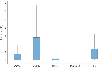
The medians as well as the Z rank reveal as PSOc and PSO-GA outperform the other competitors. The Box plot diagram at 95 percent confidence level reported in Fig. 4 confirms that there was a statistical difference among the different metaheuristics.
Fig. 4. Comparison of meta-heuristics: Boxplot
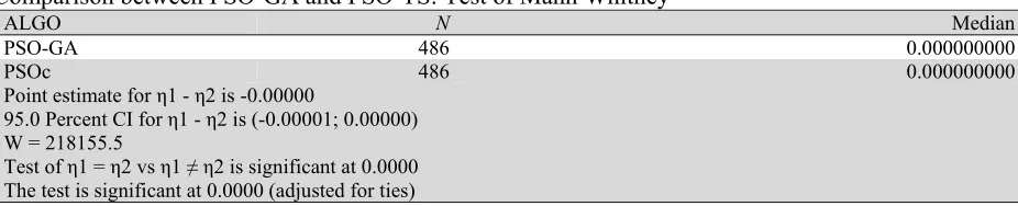
Table 13
Comparison between PSO-GA and PSO-TS: Test of Mann Whitney
ALGO N Median
PSO-GA 486 0.000000000
PSOc 486 0.000000000
Point estimate for η1 - η2 is -0.00000
95.0 Percent CI for η1 - η2 is (-0.00001; 0.00000) W = 218155.5
Test of η1 = η2 vs η1 ≠η2 is significant at 0.0000 The test is significant at 0.0000 (adjusted for ties)
6. Conclusions and Future Research
In this research, we have approached a single machine batch processing problem with release dates to minimize the total completion time (1|rj, batch|
Cj). A mathematical model has been proposed to solve the research problem optimally. The proposed research problem is known to be NP-hard; hence, several meta-heuristic algorithms based on TS and PSO with two different approaches have been developed to heuristically solve the problem. Since the normal probability plot of residuals were not normally distributed, a non-parametric test (Kruskal-Wallis) was employed to compare the performance of the proposed algorithms. The results show that there was a significant statistical difference among the meta-heuristic algorithms. Medians and Z rank demonstrate that PSOa and PSO-GA assure the most promising performances compared to the other metaheuristics. Therefore, in order to find the algorithm with the best efficiency between PSOc and PSO-GA, a post-hoc pairwise comparison based on a non-parametric Mann-Whitney U test was employed. The result of Mann-Whitney test indicates that PSO-GA had a better performance than PSOc. Since the proposed research problem was investigated in a single machine environment, the obtained results in this research can be applied in other environments such as parallel machines and flow shop. A lower bounding method can be provided to evaluate the performance of the proposed meta-heuristic algorithms for the future research.References
Al-Salamah, M. (2015). Constrained binary artificial bee colony to minimize the makespan for single machine batch processing with non-identical job sizes. Applied Soft Computing, 29, 379 -85.
Arabameri, S., & Salmasi, N. (2013). Minimization of weighted earliness and tardiness for no-wait sequence-dependent setup times flow-shop scheduling problem. Computers & Industrial Engineering, 64(4), 902-916.
Baker, R.K., & Trietsch, D. (2009). Principles of Sequencing and Scheduling; New Jersey: John Wiley & Sons.
Chandru,V., Lee, C.Y., & Uzsoy, R. (1993). Minimizing total completion time on a batch processing machine with job families. Operations Research Letters, 13(2), 61-65.
Chang, P.C., & Wang, H.M. (2004). A heuristic for a batch processing machine scheduled to minimize total completion time with non- identical job sizes. The International Journal of Advanced Manufacturing Technology, 24(7), 615-620.
Chen, Y.Y., Cheng, C.Y., Wang, L.C., & Chen, T.L. (2013). A hybrid approach based on the variable neighborhood search and particle swarm optimization for parallel machine scheduling problems: a case study for solar cell industry. International Journal of Production Economics, 141(1), 66-78. Coello Coello, C.A., Lamont, G.B., & Van Veldhuizen, D.A. (2007). Alternative Meta-heuristics:
Boston, MA: Springer US.
P. Beldar and A. Costa
Costa, A., Alfieri, A., Matta, A., & Fichera, S. (2015). A parallel tabu search for solving the primal buffer allocation problem in serial production systems. Computers & Operations Research, 64, 97-112. Costa, A., Cappadonna, F.A., & Fichera, S. (2016). Minimizing the total completion time on a parallel
machine system with tool changes. Computers & Industrial Engineering, 91, 290-301.
Costa, A., Cappadonna, F.A., & Fichera, S. (2017). A hybrid genetic algorithm for minimizing makespan in a flow-shop sequence-dependent group scheduling problem. Journal of Intelligent Manufacturing, 8(6), 1269-1283.
Damodaran, P., Manjeshwar, P.K., & Srihari, K. (2006). Minimizing makespan on a batch-processing machine with non-identical job sizes using genetic algorithms. International Journal of Production Economics, 103(2), 882-891.
Damodaran, P., Srihari, K., & Lam, S.S. (2007). Scheduling a capacitated batch-processing machine to minimize makespan. Robotics and Computer-Integrated Manufacturing, 23(2), 208-2016.
Damodaran, P., Diyadawagamage, D.A., Ghrayeb, O., & Velez-Gallego, M.C. (2012). A particle swarm optimization algorithm for minimizing makespan of non-identical parallel batch processing machines. The International Journal of Advanced Manufacturing Technology, 58(9), 1131-1140.
Dupont, L., & Dhaenens-Flipo, C. (2002). Minimizing the makespan on a batch machine with non-identical job sizes: an exact procedure. Computers & Operations Research, 29(7), 807-819.
Gao, H., Kwong, S., Fan, B., & Wang, R. (2014). A Hybrid Particle-Swarm Tabu Search Algorithm for Solving Job Shop Scheduling Problems, IEEE Transactions on Industrial Informatics, 10(4), 2044-2054.
Glover, F., & Laguna, M. (1999). Tabu Search. Boston, MA: Springer US.
Gohari, S., & Salmasi, N. (2015). Flexible flowline scheduling problem with constraints for the beginning and terminating time of processing of jobs at stages. International Journal of Computer Integrated Manufacturing, 28(10), 1092-1105.
Javidrad F., Nazari M.. (2017). A new hybrid particle swarm and simulated annealing stochastic optimization method. Applied Soft Computing, 60, 634-654.
Jia, Zh., & Leung, J.Y.T. (2014). An improved meta-heuristic for makespan minimization of a single batch machine with non-identical job sizes. Computers & Operations Research, 46, 49-58.
Jolai, F., & Dupont, L. (1997). Minimizing mean flow times criteria on a single batch processing machine with non-identical jobs sizes. International journal of production economics, 55, 273-280.
Kennedy, J., & Eberhart, R. (1995). Particle swarm optimization. In: Neural Networks, 1995 Proceedings., IEEE International Conference on, 4, 1942-1948.
Kuo, R.J., & Han, Y.S. (2011). A hybrid of genetic algorithm and particle swarm optimization for solving bi-level linear programming problem – A case study on supply chain model. Applied Mathematical Modelling, 35(8), 3905 – 3917.
Kwak, J.S. (2005). Application of taguchi and response surface methodologies for geometric error in surface grinding process. International Journal of Machine Tools and Manufacture, 45(3), 327-334. Lee, C.Y. (1999). Minimizing makespan on a single batch processing machine with dynamic job arrivals.
International Journal of Production Research, 37(1), 219-236.
Lee, Y.H., & Lee, Y.H. (2013). Minimizing makespan heuristics for scheduling a single batch machine processing machine with non-identical job sizes. International Journal of Production Research, 51(12), 3488-3500.
Li, Z., Chen, H., Xu, R., & Li, X. (2015). Earliness–tardiness minimization on scheduling a batch processing machine with non-identical job sizes. Computers & Industrial Engineering, 87, 590-599. Liao, L.M., & Huang, C.J. (2011). Tabu search heuristic for two-machine flowshop with batch processing
machines. Computers & Industrial Engineering, 60(3), 426-432.
Lin, H., & Kang L. (1999). Balance between exploration and exploitation in genetic search, Wuhan University Journal of Natural Sciences, 4(1), 28–32.
Liu, Z., & Yu, W. (2000). Scheduling one batch processor subject to job release dates. Discrete Applied Mathematics, 105(13), 129-136.
Melouk, S., Damodaran, P., & Chang, P.Y. (2004). Minimizing makespan for single machine batch processing with non-identical job sizes using simulated annealing. International Journal of Production Economics, 87(2), 141-147.
Michalewicz, Z. (1996). Genetic Algorithms + Data Structures = Evolution Programs. Springer Science & Business Media.
Parsa, N.R., Karimi, B., & Kashan, A.H. (2010). A branch and price algorithm to minimize makespan on a single batch processing machine with non-identical job sizes. Computers & Operations Research, 37(10), 1720-1730.
Parsa, N. R., Karimi, B., & Husseini, S. M. (2016). Minimizing total flow time on a batch processing machine using a hybrid max–min ant system. Computers & Industrial Engineering, 99, 372-381.
Poli, R., Kennedy, J., & Blackwell, T. (2007). Particle swarm optimization. Swarm Intelligence, 1(1), 33-57.
Raymond, H.M., Douglas, C.M., & Christine, M. AC. (2009). Response Surface Methodology: Process and Product Optimization Using Designed Experiments. New Jersey: John Wiley & Sons.
Sha, D.Y., Hsu, C.-Y. (2006). A hybrid particle swarm optimization for job shop scheduling problem. Computers & Industrial Engineering, 51(4), 791-808.
Shi, Y., & Eberhart, R.C. (1950). Empirical study of particle swarm optimization. In: Proceedings of the 1999 Congress on Evolutionary Computation-CEC99 (Cat. No. 99TH8406), 3, 1950 vol. 3.
Simon, D. (2013). Evolutionary Optimization Algorithms; New Jersey: John Wiley & Sons.
Tadayon, B., & Salmasi, N. (2013). A two-criteria objective function flexible flowshop scheduling problem with machine eligibility constraint. The International Journal of Advanced Manufacturing Technology, 64(5), 1001-1015.
Uzsoy, R. (1994). Scheduling a single batch processing machine with non-identical job sizes. International Journal of Production Research, 32(7), 1615-1635.
Uzsoy, R., & Yang, Y. (1997). Minimizing total weighted completion time on a single batch processing machine. Production and Operations Management, 6(1), 57-73.
Xia, W.-J., & Wu, Z.-M. (2006). A hybrid particle swarm optimization approach for the job-shop scheduling problem. International Journal of Advanced Manufacturing Technology, 29(3–4), 360– 366.
Xu, R., Chen, H., & Li, X. (2012). Makespan minimization on single batch-processing machine via ant colony optimization. Computers & Operations Research, 39(3), 582-593.
Zhou, S., Chen, H., Xu, R., Li, X. (2014). Minimizing makespan on a single batch processing machine with dynamic job arrivals and non-identical job sizes. International Journal of Production Research, 52(8), 2258-2274.