Pricing and lot sizing optimization in a two-echelon supply chain with a constrained Logit demand function Pages 205-220 Download PDF

(1)

* Corresponding author

E-mail: [email protected] (H. López-Ospina)

International Journal of Industrial Engineering Computations 9 (2018) 205–220

Contents lists available at GrowingScience

International Journal of Industrial Engineering Computations

homepage: www.GrowingScience.com/ijiec

Pricing and lot sizing optimization in a two-echelon supply chain with a constrained

Logit demand function

Yeison Díaz-Mateusa_{, Bibiana Forero}a_{, Héctor López-Ospina}b*_{and Gabriel Zambrano-Rey}a

a_{Industrial Engineering Department, Pontificia Universidad Javeriana, Cra 7 #40-62, Ed. Jose Gabriel Maldonado P.3, Bogotá, Colombia} b_{Department of Industrial Engineering, Universidad del Norte, Km. 5 Vía Puerto Colombia, Barranquilla, Colombia}

C H R O N I C L E A B S T R A C T Article history:

Received February 13 2017 Received in Revised Format April 1 2017

Accepted June 16 2017 Available online June 16 2017

Decision making in supply chains is influenced by demand variations, and hence sales, purchase orders and inventory levels are therefore concerned. This paper presents a non-linear optimization model for a two-echelon supply chain, for a unique product. In addition, the model includes the consumers’ maximum willingness to pay, taking socioeconomic differences into account. To do so, the constrained multinomial logit for discrete choices is used to estimate demand levels. Then, a metaheuristic approach based on particle swarm optimization is proposed to determine the optimal product sales price and inventory coordination variables. To validate the proposed model, a supply chain of a technological product was chosen and three scenarios are analyzed: discounts, demand segmentation and demand overestimation. Results are analyzed on the basis of profits, lotsizing and inventory turnover and market share. It can be concluded that the maximum willingness to pay must be taken into consideration, otherwise fictitious profits may mislead decision making, and although the market share would seem to improve, overall profits are not in fact necessarily better.

Constrained multinomial logit Pricing

Lotsizing

Supply chain optimization PSO

1. Introduction

(2)

models have introduced specific conditions such as discounts (Berger & Bechwati 2001), payment due dates (Ghoreishi, et al., 2014), and segmentation of demand (Ghoniem & Maddah 2015). On the other hand, Shavandi et al. (2012) present a constrained multi-product pricing and inventory model in which perishable products are put into three categories: substitute, complementary and independent; to solve the model genetic algorithm is developed. However, it is important to note that in most of these studies, the demand is modeled with linear and price elasticity functions, which do not necessarily capture all key aspects in the customers purchase behavior. Then, this paper proposes a model that incorporates the changes in demand and its influence on the price adjustment and on the logistic costs associated with inventory levels, in a coordinated problem between a supplier and a vendor. Also, the model considers that there are different socioeconomic groups with different product valuation, hence with different maximum willingness to pay. For the proposed model, the I-JPLMSP model (Yaghin et al., 2014)

(Integrated join pricing and lotsizing model with sales promotions) is taken as reference because it

integrates the level of inventories with the optimal price in a two echelon supply chain, and also it includes discount and sales policies to meet demand. This logistic model assumes a single vendor and supplier, and a unique non-perishable product without seasonality, with an infinite production rate. However, the I-JPLMSP model is built upon a non-linear function of demand based on a multinomial logit distribution (MNL) (Márquez-Díaz et al., 2011). Thus, demand is only evaluated for a single group of customers with the same rating for the product attributes. The I-JPLMSP model aims is to optimize the multi-echelon profits between the vendor and the supplier.

The main contribution of this paper is to extend the I-JPLMSP model to take into account the following conditions. First, customer segmentation to analyze different socioeconomic groups, with different product valuations, for obtaining a more appropriate demand estimation. Second, price constraints are introduced by using the constrained multinomial logit (CMNL) (Martínez et al., 2009) instead of the unconstrained multinomial logit. The main advantage of using the CMNL over traditional MNL is the possibility to include constraints on the product’s attributes through penalty functions (Pérez et al., 2016). In particular, the CMNL allows to include a constraint associated with the maximum willingness to pay by customers that directly affects the estimation of demand and optimal price. Finally, to validate the model, a case study in the Colombian market was used, where socio-economic segmentation is quite present and has an impact on demand and product price estimation.

The rest of the paper is organized as follows. Section 2 explains the CMNL for demand estimation. Then, Section 3 starts by presenting the problem statement, and then the formulation of demand based on the CMNL is explained, followed by the formulation of the logistic multi-echelon model, and last by the Model resolution procedure.

2. The constrained multinomial logit for demand estimation

In this research, the discrete choice model known as constrained multinomial logit (CMNL) is used (Martínez et al., 2009) to include constraints on the product selling price, taking into account the consumers’ maximum willingness to pay. The CMNL assumes that the perceived utility by an agent, i.e., a consumer, who belongs to the socio-economic group (h) associated with the discrete product (x) denoted by is split into a compensatory part (a in Eq. (1)) and another non-compensatory part (b in Eq. (1)) which indicates the feasibility of that alternative to h,

(3)

Y. Díaz-Mateus et al. / International Journal of Industrial Engineering Computations 9 (2018)

where is a boundary or penalty function imposed by group h to the attributes of the discrete product x. The stated penalty, with a logarithm function, allows constraints to be subtly broken by the decision maker (Martínez et al., 2009). The random component represents and reflects the inability of the analyst to model all the attributes and changes in preferences and behaviors of individuals, measurement and modeling errors, lack of accurate information, among others. If such inaccuracies are Gumbel distributed with scale parameter , then the probability of a consumer, who belongs to group (h), to purchase product I can be represented as in equation (2).

℮

1 ∑ ℮ . ∀ ∈

(2)

This probability is known as the constrained multinomial logit model (CMNL) (Martínez et al., 2009). There are some interesting and novel applications that are used on modeling demand in a discrete choices context, in areas such as the mode of transport choice (Castro, et al., 2013), the location of schools and their capacity (Castillo-López & López-Ospina 2015; Martinez, et al., 2011), the optimal price and packaging (Pérez et al., 2016), the subway route choice (Herrera, 2014), place of residence and housing choice (Martínez & Donoso 2010; López-Ospina, et al., 2016; López-Ospina, et al., 2017 ), food choice (Ding et al., 2012), parking management (Caicedo, et al., 2016) among others. These applications require constrained variables in different contexts, which imply high non-linearity in demand estimation, which also involves high non-linearity when attributes are decision variables within optimization models, such as the selling price. The following sections describe the detailed logistic problem and the non-linear formulation proposed.

3. The logistic non-linear optimization problem

3.1Problem statement

The problem modeled in this article is focused on a two-echelon supply chain with a single vendor and a single supplier, trading a single non-perishable product under the assumption of coordination of cycle times for both supplier and vendor. To formulate the problem the following parameters and variables are taken into account:

Parameters

, ∈

Variables

′ _′ _.

′

(4)

Assumptions

 The maximum willingness to pay, that each group h assigns to the product, is known

 The inventory replenishment time is negligible

 Planning time is infinite

 The supplier delivery rate is infinite

 There is a coordination of inventory cycle times between the vendor and the supplier

3.2. Formulation of demand based on the CMNL

From the point of view of microeconomic modeling, discrete choice analysis on a product is based on the principle of utility maximization where the price is directly related to observable characteristics of the product. In addition, it is assumed that each individual makes the decision based on the perceived utility of the product, good or service. Hence, this situation can be modeled by random utility models (RUM) initially developed by Block and Marschak (1960). In 1975, Mc Fadden (1975) makes an econometric extension of this theory by considering that a population of individuals do the same choice on a set of alternatives, i.e., that the population can be split up having as a reference common socio-economic factors in a group of individuals which conditions their choices. Each group h within the population is called cluster (Martínez et al., 2009). A particular case of these models is the multinomial logit, used by Yaghin et al. (2014) to estimate demand D, under the assumption of a single socio-economic group (H=1), as in equation (3).

℮

1 ℮ , , 0

(3)

In Eq. (3) the utility function is given by , assuming a single product valuation attribute, i.e., the price P, and its coefficient of variation -b, that shows the variation per price unit changed in the utility function. The utility function is negative because for any consumer, an increase in the product price decreases its perceived utility. In addition, the market size is represented by , which allows to obtain a deterministic demand since the demand for that product, at price P, can be obtained by multiplying the number of customers by the purchase probability.

This paper proposes a new model for demand estimation, but using the constrained multinomial logit (CMNL), and introducing the following aspects that make demand estimation more realistic: 1. multiple socio-economic groups with similar characteristics to consumers from the same group in order to analyze and describe logistic and demand impacts. It is important to clarify that an aggregate demand will be obtained, that is, the sum of demands for all clusters. 2. The utility function associated with the product depends on the product selling price P and on a set of characteristics , 1,2, … , that defines product attractiveness, which are assessed for each sub-group h, as suggested in equation (4).

∀ ∈ (4)

In Eq. (4), are the coefficients associated with each characteristic k of the product, within characteristics assessed by group h. Therefore, if it is assumed that the error is independent and identically distributed (IID) Gumbel with scale parameter . Then, if is introduced in Eq. (3) replacing

V, the demand for each group or cluster h for the product is defined as:

℮ ∑

1 ℮ ∑ , ∀ ∈

(5)

Hence, the aggregate demand can be calculated as:

(6)

Based on Eq. (5), the probability of not purchasing for each group h is defined as:

probability of not purchasing 1

1 ℮ ∑ , ∀ ∈

(7)

A third aspect that is integrated to this model is a penalty associated with the maximum willingness to pay for the product, for each group h; making demand estimation more realistic. Thus, demand modeling changes from the classic multinomial logit model to the discrete choice model known as CMNL (Eq. 8).

℮

1 ℮ . ∀ ∈

(8)

Therefore, the perceived utility presented in Eq. (4) becomes Eq. (9) to introduce the maximum willingness to pay for the product, for each group h, denoted as ln and an exogenous lower

bound for the product price . These two constraints are defined by a binomial logit model (Castro et al., 2012) (Eq. (11) and Eq. 12), so that each subgroup h can delimit the product choice based on price. The CMNL allows to smoothly integrate those constrains.

1

ln 1 ∀ ∈ (9)

(10)

1 1

(11)

1

1 .

(12)

In Eqs. (11-12), and are the lower and upper bounds for the product’s price, respectively, is the scale parameter of the binomial logit, and is a parameter defined by Eq. (13), that includes as the value associated with the population’s proportion that overrides the associated constraint. It is important to note that if the parameter is set to 0 or 1, then the given expression for is undefined, because the binominal logit functions can only predict deterministic choices (probabilities equal to zero or one) when the variables tend to infinity (Martínez et al., 2009).

1 ln

1

. (13)

Once the new demand function is defined with the inclusion of the new conditions, the following section shows how this demand is used in a logistic model.

3.3. Formulation of the logistic multi-echelon model

(6)

. (14)

For this model, it is assumed that the vendor is a retailer that purchases the product and resale it. For this reason its total annual profit function, depending on the estimated aggregated demand, is described as follows:

∑ 0,5 ∑ ∑ . ₍₁₅₎

For the supplier, it is assumed that it is a wholesaler who purchases a product to market it though its distribution channels and make a profit. Thus, an EOQ (economic order quantity) model is assumed resulting in a profit function similar to the vendor's, but with the following differences: (1) supplier profit is calculated based on the vendor purchase price; (2) a formulation (Eq. (16)) was used to coordinate inventories based on reorder time of the supplier, to avoid inventory shortages in the model

. (16)

Then, the joint utility function under the assumption of coordination between the two echelons of the supply chain is described by Eq. (17).

, , , , ∑ 0,5 1 ∑ ∑

0,5 ∑

∑ .

(17)

3.4. Model resolution procedure

The proposed logistic model implies a high non-linearity in estimating demand, where there is a direct relationship, and non-linear, between the restricted demand and the logistic model choices. Consequently, it is not possible to obtain a solution analytically or using an exact method, and therefore heuristics and meta-heuristics must be used. Given that PSO (particle swarm optimization) has shown the effectiveness in highly non-linear optimization problems (Moghadam & Seyedhosseini, 2010; Hashemi, et al., 2010; Zahara & Hu, 2008; Xu et al., 2013; Jafari et al., 2013; Karimi-Nasab, et al., 2015; Bai et al., 2016; Kumar, et al., 2016, Guedria, 2016; among others), in this work a PSO was used to solve the logistic model. The Eq. (19) and Eq. (18) show the velocity and position of each particle i for each dimension d

at iteration t, where is the particle inertia, and are acceleration constants, is the best position the particle has reached to the current iteration, and is the position of the best particle of the whole swarm, considering a fully connected swarm (Kennedy & Mendes 2002). Fig. 1 shows the resolution procedure pseudo-code.

∗ 1 ∗ ∗ 1

∗ ∗ 1 , (18)

1 . (19)

(7)

Fig 1. Resolution procedure based on PSO

Eq. (17) is used as the PSO objective function, and for each variable the following feasibility constraints are true as it is explained below.

Feasibility constraint for m

To analyze this constraint, it is assumed that variable m is continuous, thus the first derivate of Eq. (17) regarding m is defined as:

0,5 1

0,5 ,

(20)

then:

0,5 . (21)

Therefore, a critical point of the function is found, obtaining:

√2

∑ 2 .

(22)

Analyzing the second derivative regarding m:

2

. (23)

Since the second derivative is negative, then the critical point is a relative maximum. Through Eq. (22), it can be stated that is a non-decreasing function of P. Thus, the maximum number of shipments can be set as

Define particle’s dimensions

Define the feasible space for each dimension Set swarm size, c1, c2, 

Do {

Initialize randomly each particle’s position (feasible space) Initialize randomly each particle’s velocity (feasible space) Calculate each particle’s fitness (calculate demand()) Besti=current particle’s position

} for all particles in the swarm Bestg=best particle

Do {

Calculate each particle’s new velocity (feasible space) Calculate each particle’s new position (feasible space) Calculate each particle’s fitness(calculate demand()) Besti=current particle’s position

} for all particles in the swarm Bestg=best particle

} While the max number of iterations is not attained

(8)

 → 0 → 0,1

 → , . ∑ → 0

0,1 ∗ .

(24)

Thus it can be concluded that the maximum value of the profit function is associated with an integer value m in the interval 1, .

Feasibility constraint for

assumes a lower and an upper level of duration, which depends on market dynamics and product obsolescence. As a result, strongly depends on the chosen market and product that are evaluated on the proposed model, considering that ≠0.

Feasibility constraint for P

Within the logistic model a purchase price was established for the vendor, which is defined as the lower bound of the price P, and the upper bound of the price is given by the maximum willingness to pay among all socio-economic groups h. Taken into account that the CMNL allows the price not to strictly respect these constraints, by a soft penalty (as shown in Fig. 2), hard upper and lower bounds were established for the PSO, up to half of the purchase price (lower bound, Cv/2) and to double of the maximum willingness to pay among all socio-economic groups (upper bound, 2*max{ah}).

Fig 2. Penalty functions of constrained Logit

4. Implementation and results

To validate the proposed model the digital television market was chosen, particularly in the Colombian context, based on the previous study of González and Serna (2013). From this work, the 32-inch LED television was taken as the reference because of its variance in demand. Only in 2013, 1'700.000 screens were sold in the country, and in 2014 the sales of these products were around 2 million units. As far as the sizes, 32-inch models are consolidated as the preferred size by Colombians with more than 52% of sales, and LED technology accounts for 90% of sales (Tiempo, 2016a; Tiempo, 2016b). In the following sections, the socio-economic groups, costs, and logit parameters are defined, and the implementation procedure and results analysis are reported.

4.1. Socio-economic groups and attributes definition

(9)

From the obtained results, an analysis of variance was performed from which it was concluded, with a significance level of 5%, that the single studied variable that affects the maximum willingness to pay is the socio-economic group to which the individual belongs. Additionally, to define the upper and lower bound constraints, the maximum willingness to pay for each socio-economic group and the market size (193436 inhabitants) based on the target population defined by surveys were obtained. Such values are presented in Table 1.

Table 1

Socio-economic groups

Socio-economic groups Maximum willingness to pay (COP$)

1 dollar is equivalent to 3000 COP$ Market size (inhabitants)

Lower 894.615 50 294

Middle 1.190.604 115 288

Upper 1.958.333 27855

From these results, the price sensitivity coefficient is also defined as shown in Table 2. Table 2

Price sensitivity coefficient

Socio-economic groups Price sensitivity coefficient

Lower 0.725

Middle 0.5375

Upper 0.225

Finally, through direct observation of the market, the minimum selling price of 32-inches LED televisions is set to COP$ 620.999.

4.2. Costs definition

Because the costs associated in Eq. (17) are strategic values of enterprises and therefore is not readily available information, additional parameters were included so such values could be estimated. Then, the parameter PV was included and it refers to the average current selling price in the market, COP$ 927.104. As well, the parameter PG was included to represent the expected profit percentage. Three reference values of 30%, 40 and 50% were fixed for PG. The parameter PV is equal to both supplier and vendor, as the logistic model aims to balance the perceived profits for the two echelons in the chain. Consequently, to set the values of and the relationship between the vendor and supplier was defined as shown in Fig. 3.

Fig 3. Relationship between vendor and supplier costs

Similarly, the costs of holding inventory and ordering were defined under the established relationships in Table 3.

Table 3

Holding inventory costs and ordering costs for vendor and supplier

Cost Relation

Vendor Holding 0,15 times

Ordering 41,67 times

Supplier Holding 0,08 times

(10)

4.3. Parameters for the CMNL

As proposed by Castro et al. (2013),the penalty is defined as the product of both, the upper and lower constraints. Taking into account that both constraints and their thresholds are independent, the results of constraints by varying the parameters and ( ) in Eqs. (11-13) were analyzed. Then, it was evident that the penalties were too strict when took values lower than 0.9, and after this value, variations were not significant. In addition, it was noted that the more increased, there were not large variations. For this reason, it was established that an intermediate penalty would be used, for which . was fixed.

4.4. Procedure implementation

The implementation of the proposed model was run on R Statistics software. To implement the solution, and based on some control instances, the parameters in Table 4 were used, which allowed convergence of the model.

Table 4

Values for PSO parameters

Parameters Values

Par (Components of each individual) Empty array of length 3

Fn (Adaptability function) Joint gains function equation (17)

Lower (Lower constraints) Array containing lower bounds for each variable

Upper(Upper constraints) Array containing upper bounds for each variable

Maxit (Number of iterations) 1500

S (Population size) 60

W (Decreasing inertia) Minimum value: 0,02

Maximum value: 2

4.5. Results analysis

Given the general description of the optimization problem, the proposed model was evaluated against three scenarios. The first scenario analyzes the impact of discounts by means of sensitivity analysis. The second scenario compares the model without including the price constraints in the logit demand function. More, to obtain an approach that depicts the influence of customer behavior in demand estimation, a third scenario including socio-economic segmented demand was assessed. In order to assess the model accuracy and its behavior in the proposed scenarios, the base model was considered regardless of the product attractiveness, i.e., assessment of the attributes other than price in the utility function. Hence, the analysis of the base model and product attractiveness are presented at first, followed by the scenarios.

Analysis of the base model

Results obtained from the base model are reported in Table 5. When performing a comparative analysis among the three expected profit percentages, it can be noted that the biggest profit obtained was when

(11)

phenomenon is associated to holding inventory costs, since the more the duration of inventory increases for the vendor and supplier, the lower the expected profit percentage. Finally, when comparing the average price obtained by direct observation of the market ($ 927,104) to the three studied values, the model that gets closest to this number is the model with PG=50%. For this reason, an expected profit of 50% was used for the following analysis.

Table 5

Results of base model

Parameters PG=30% PG=40% PG=50%

Objective Function (COP$) 24,171,500,000 29,250,350,000 33,720,110,000

Price (COP $) 1,079,779 1,050,611 1,030,514

Number of shipments within one supplier’s cycle 2 2 2

Duration of vendor’s inventory (days) 55 54 53

Number of shipments per year 7 7 7

Duration of supplier’s inventory (days) 110 107 106

Q 6023 6159 6243

Demand 40081 41903 43050

Total costs for vendor (COP $) 6,484,300,000 23,723,450,000 20,305,930,000

Total costs for supplier (COP $) 18,634,300,000 14,359,020,000 10,293,500,000

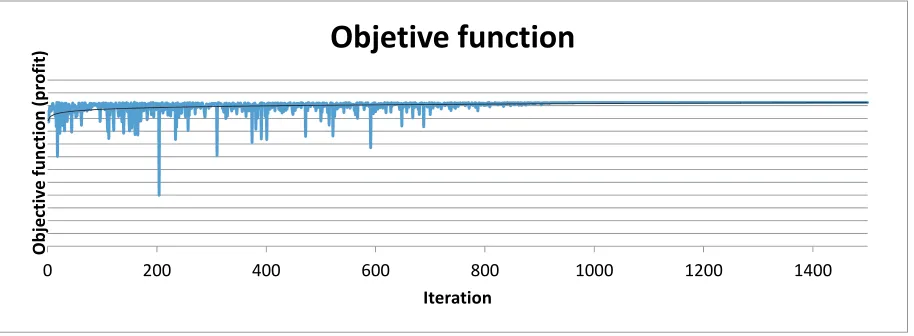
To observe the behavior of PSO throughout iterations, the convergence curve for the objective function for the case of an expected profit set to 50% is shown in Fig. 4.

Fig 4. Convergence chart for base model

Analysis of product attractiveness

To analyze product attractiveness, a sensibility analysis study on two factors was conducted: socio-economic group and attractiveness, each of them with three levels (lower, middle, upper), being the price the response variable.

Table 6

Sensibility analysis

Analysis of variance

Origin of variations Sums of squares (COP$) Degrees of freedom Average of squares F P-value

Social stratum (E) 6,484,778,577,204 2 8.24E+12 1.49E+06 0.00%

Attraction (A) 9,750,856,924 2 4.88E+09 8.83E+02 0.00%

E&A 2,409,729,336 4 6.02E+08 1.09E+02 0.00%

Error 1,590,787,406 288 5.52E+06

Total 16,498,529,950,870 296 5.57E+10

5%

0 200 400 600 800 1000 1200 1400

Ob

je

ct

iv

e

functio

n

(profit)

Iteration

(12)

All possible values of attractiveness were evaluated within the intervals defined above and 33 results were obtained for each possible combination between the levels of social stratification and product attractiveness. Once these data obtained, an analysis of variance was performed as shown in Table 6. With a significance level of 5% it was evident that social stratification, product attractiveness and the combination of both factors significantly affect the optimal price, and therefore, they also affect significantly the entire logistic model. Based on the adjusted coefficient of determination, it was found that 99.9% of the observed price variation is explained by the model. Given the above results, it can be noted that product attractiveness becomes relevant in this model for both price definition and inventory management. Nevertheless, it was stated that attractiveness would be equal to 0 in the following analysis, i.e., the utility function depends only on the price variable, similar to the model developed on the model I-JPLMSP designed and analyzed by Yaghin et al. (2014).

4.5.1. Scenario 1: Discounts analysis

In order to analyze the logistic impact by incorporating the sales discounts (r), r is defined based on the expected profit percentage (PG). To avoid losses, the following relationships were established among the selling price found in the market (including discounts) and the purchase cost of vendor:

∗ 1 (25)

1 1

(26)

Thus:

(27)

Then, the utility function of CMNL model was adjusted as shown in equations (28)-(30)

1 ∀ ∈ (28)

℮

1 ℮ ∀ ∈

(29)

, , , , 1 0,5 1

0,5

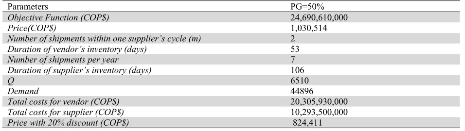
(30) Finally, based on an expected profit of 50% (upper bound) and on direct market observation, it was established that the most common discount on the selling price is 20%, as reported in Table 7. From these results it is noted that by incorporating the discount, all the associated parameters are affected, especially the demand and profits. With a 20% discount, demand increased 4.29% with respect to base model, but the total profit decreased by 36.6%.

Table 7

Results for 20 % discount

Parameters PG=50%

Objective Function (COP$) 24,690,610,000

Price(COP$) 1,030,514

Number of shipments within one supplier’s cycle (m) 2

Duration of vendor’s inventory (days) 53

Number of shipments per year 7

Duration of supplier’s inventory (days) 106

Q 6510

Demand 44896

Total costs for vendor (COP$) 20,305,930,000

Total costs for supplier (COP$) 10,293,500,000

(13)

4.5.2. Scenario 2: Logit model

The objective of this scenario was to analyze the impact of constraints and hence, these were omitted in the calculation of demand with the classical MNL. The results of this scenario are shown in Table 8. From those, it can be observed that by not considering the constraints in the model, demand was overestimated at 26.8% compared to the base model. In turn, this overestimation means that profit increases 4 times above the base model. Additionally, it is evident that price tended to the upper bound imposed, so that for a product such as 32-inch LED television, a high price that is 4,2 times the one found in the market was held.

Table 8

Results of Logit model

Parameters PG=50%

Objective Function (COP$) 200,486,000,000

Price (COP$) $ 3,916,667

Number of shipments within one supplier’s cycle (m) 2

Duration of vendor’s inventory (days) 47

Number of shipments per year 8

Duration of supplier’s inventory (days) 94

Q 7031

Demand 54611

Total costs for vendor (COP$) 25,709,260,000

Total costs for supplier (COP$) 3,012,920,000

4.5.3. Scenario 3: Segmented demand

In order to analyze the influence and logistic impacts of each socio-economic group defined within the demand, a model was run for each group, taking into account a product attractiveness equal to 0, an expected profit equal to 50% and an estimated demand through the CMNL. The results obtained are presented in Table 9. Meanwhile, Table 10 shows the contribution of each socio-economic group to the aggregate demand of the base model. From these results it can be noted that, as for the base model, the greatest demand is associated to middle-stratum, followed by the lower-stratum and finally by the upper-stratum. This demand behavior is explained due to the distribution of the surveyed population, since 26% corresponds to lower-social stratum, 59.6% to middle-stratum, and 14.4% to upper-stratum. Furthermore, it is noted that demand for each group varies in different proportions in relation to the selling price, and therefore, by taking the price of the base model as a reference, it was evident that price decreased by 7% in lower-stratum, and demand increased by 12%. For middle-social stratum, price increased 1% and consequently demand decreased 1.4%. For the latter group, the upper-social stratum, the price increased by 26% and demand decreased by 7%.

Table 9

Results for aggregate demand

Parameters Lower Middle Upper

Objective Function (COP$) $ 912,741,000 $ 22,901,800,000 $ 1,457,199,000

Price (COP$) $ 962,381 $ 1,042,319 $ 1,386,959

Number of shipments within one supplier’s cycle 2 2 2

Duration of vendor’s inventory (days) 93 65 297

Number of shipments per year 4 6 1.2

Duration of supplier’s inventory (days) 185 129 595

Q 3571 5117 823

Demand 14089 28928 1010

Total costs for vendor (COP$) $ ,731,220,000 $ 13,696,550,000 $ 694,587,900

(14)

Regarding the duration of supplier's inventory, it can be observed that an order is made every 297 days for the upper-social stratum in order to meet their demand, being its inventory cycle of 595 days. This long duration may significantly affect the devaluation of inventory, meaning that as time passes the monetary unit will lose their commercial value because of technology advances, which significantly impact the televisions market, with high risk of technology obsolescence.

Finally it is noted that the target population is located at middle-social stratum since this stratum contributes 65.7% of total demand. For this reason, and to facilitate comparison among different the proposed scenarios, the impact of this scenario was assessed only by using the middle-stratum.

Table 10

Influence of groups on aggregate demand

Sub-groups Lower Middle Upper

PG= 50% 12623 29341 1086

5. Conclusions

This paper has presented a logistic optimization, non-linear, multi-echelon model that integrates the selling price of a product and the level of inventories, including a constraint about the maximum willingness to pay of customers, taking into account different socio-economic groups. To estimate the demand, the discrete choice multinomial restricted logit (CMNL) model was used in order to include soft constraints on the purchase price. Moreover, the optimal purchase price, as well as the coordination inventory variables, were obtained through a metaheuristic based on particle swarm optimization (PSO).

To validate the proposed model, the population was segmented into lower, middle and upper classes depending on their income, according to the Colombian social stratification. In assessing the behavior of each socio-economic group faced to the choice of the same product, the choice is conditioned by the maximum willingness to pay. In contrast, from the vendor's perspective it is important to consider the minimum selling price. Therefore, there is a need to use the constrained multinomial logit model for modeling demand, in order to include the aforementioned constraints.

Through the application example, the behavior of the proposed aggregate demand model could be analyzed against three scenarios. The first scenario focused on the base model with a sensitivity analysis on possible discounts, the second scenario estimated demand by means of a non-constrained multinomial logit model and the third scenario contemplated a segmented demand for each socio-economic group. From the first scenario, it was observed that when considering a discounts policy based on the vendor’s expected profit, discounts increased market share but not necessarily generated higher profits compared to those obtained with the base model. That is, the value of the objective function decreased, compared to the base model, and in turn, demand showed an increase which can be taken as a growth strategy to increase market share in the long term.

(15)

vendor and on the socio-economic environment where it is found, aimed to establish different prices that are aligned with the highest willingness to pay of the socio-economic group. Finally, future work may be focused on expanding the model to integrate multiple products, multiple vendors and/or suppliers, and to include independent prices for each vendor.

References

Ardjmand, E., Weckman, G. R., Young, W. A., Sanei Bajgiran, O., & Aminipour, B. (2016). A robust

optimisation model for production planning and pricing under demand uncertainty. International

Journal of Production Research, 54(13), 3885-3905.

Bai, T., Kan, Y. B., Chang, J. X., Huang, Q., & Chang, F. J. (2017). Fusing feasible search space into

PSO for multi-objective cascade reservoir optimization. Applied Soft Computing, 51, 328-340.

Berger, P. D., & Bechwati, N. N. (2001). The allocation of promotion budget to maximize customer

equity. Omega, 29(1), 49-61.

Block, H. D., & Marschak, J. (1960). Random orderings and stochastic theories of

responses. Contributions to probability and statistics, 2, 97-132.

Bogotá, A. M. (2003). CARACTERIZACIÓN SOCIOECONÓMICA DE BOGOTÁ Y LA REGIÓN– V8.

Caicedo, F., Lopez-Ospina, H., & Pablo-Malagrida, R. (2016). Environmental repercussions of parking

demand management strategies using a constrained logit model. Transportation Research Part D:

Transport and Environment, 48, 125-140.

Castillo-López, I., & López-Ospina, H. A. (2015). School location and capacity modification considering

the existence of externalities in students school choice. Computers & Industrial Engineering, 80,

284-294.

Castro, M., Martínez, F., & Munizaga, M. A. (2013). Estimation of a constrained multinomial logit

model. Transportation, 40(3), 563-581.

Chen, M., & Chen, Z. L. (2015). Recent developments in dynamic pricing research: multiple products,

competition, and limited demand information. Production and Operations Management, 24(5),

704-731.

Deng, S., & Yano, C. A. (2006). Joint production and pricing decisions with setup costs and capacity

constraints. Management Science, 52(5), 741-756.

Ding, Y., Veeman, M. M., & Adamowicz, W. L. (2012). The influence of attribute cutoffs on consumers'

choices of a functional food. European Review of Agricultural Economics, 39(5), 745-769.

Geunes, J., Romeijn, H. E., & Taaffe, K. (2006). Requirements planning with pricing and order selection

flexibility. Operations Research, 54(2), 394-401.

Ghoniem, A., & Maddah, B. (2015). Integrated retail decisions with multiple selling periods and

customer segments: optimization and insights. Omega, 55, 38-52.

Ghoreishi, M., Weber, G. W., & Mirzazadeh, A. (2015). An inventory model for non-instantaneous deteriorating items with partial backlogging, permissible delay in payments, inflation-and selling

price-dependent demand and customer returns. Annals of Operations Research, 226(1), 221-238.

González, C., & Serna, N. (2013). The consumer's choice among television displays: A multinomial logit

approach. Lecturas de Economía, (79), 199-228.

Guedria, N. B. (2016). Improved accelerated PSO algorithm for mechanical engineering optimization

problems. Applied Soft Computing, 40, 455-467.

Hashemi, S. M., Rezapour, M., & Moradi, A. (2010). An effective hybrid PSO-based algorithm for

planning UMTS terrestrial access networks. Engineering Optimization, 42(3), 241-251.

Herrera Rojas, C. (2014). Desarrollo de un modelo de elección de ruta en metro. Master thesis.

Universidad de Chile.

Van den Heuvel, W., & Wagelmans, A. P. (2006). A polynomial time algorithm for a deterministic joint

pricing and inventory model. European Journal of Operational Research, 170(2), 463-480.

Jafari, H., Soltani, A., & Soltani, M. (2013). Measuring the performance of FCM versus PSO for fuzzy

(16)

Karimi-Nasab, M., Modarres, M., & Seyedhoseini, S. M. (2015). A self-adaptive PSO for joint lot sizing

and job shop scheduling with compressible process times. Applied Soft Computing, 27, 137-147.

Kennedy, J., & Mendes, R. (2002). Population structure and particle swarm performance. In Evolutionary

Computation, 2002. CEC'02. Proceedings of the 2002 Congress on (Vol. 2, pp. 1671-1676). IEEE. Kim, D., & Lee, W. J. (1998). Optimal joint pricing and lot sizing with fixed and variable

capacity. European Journal of Operational Research, 109(1), 212-227.

Kumar, E. V., Raaja, G. S., & Jerome, J. (2016). Adaptive PSO for optimal LQR tracking control of 2

DoF laboratory helicopter. Applied Soft Computing, 41, 77-90.

López-Ospina, H. A., Martínez, F. J., & Cortés, C. E. (2016). Microeconomic model of residential

location incorporating life cycle and social expectations. Computers, Environment and Urban

Systems, 55, 33-43.

López-Ospina, H. A., Cortés, C. E., & Martínez, F. J. (2017). Residential relocation dynamics: A

microeconomic model based on agents’ socioeconomic change and learning. The Journal of

Mathematical Sociology, 41(1), 46-61.

Márquez-Díaz, L. G., Gallo-González, L. A., & Chacón-Pérez, C. A. (2011). Influence of Parking Costs

on the Use of Cars in Bogota. Ingeniería y Universidad, 15(1), 105-124.

Martínez, F., Aguila, F., & Hurtubia, R. (2009). The constrained multinomial logit: A semi-compensatory

choice model. Transportation Research Part B: Methodological, 43(3), 365-377.

Martínez, F., & Donoso, P. (2010). The MUSSA II land use auction equilibrium model. In Residential

Location Choice (pp. 99-113). Springer Berlin Heidelberg.

Martinez, F. J., Tamblay, L., & Weintraub, A. (2011). School locations and vacancies: a constrained logit

equilibrium model. Environment and Planning A, 43(8), 1853-1874.

Moghadam, B., & Seyedhosseini, S. (2010). A particle swarm approach to solve vehicle routing problem

with uncertain demand: A drug distribution case study. International Journal of Industrial

Engineering Computations, 1(1), 55-64.

McFadden, D. (1975). The revealed preferences of a government bureaucracy: Theory. The Bell Journal

of Economics, 401-416.

Perez, J., Lopez-Ospina, H., Cataldo, A., & Ferrer, J. C. (2016). Pricing and composition of bundles with

constrained multinomial logit. International Journal of Production Research, 54(13), 3994-4007.

Shavandi, H., Mahlooji, H., & Nosratian, N. E. (2012). A constrained multi-product pricing and inventory

control problem. Applied Soft Computing, 12(8), 2454-2461.

Taleizadeh, A. A., & Noori-daryan, M. (2016). Pricing, manufacturing and inventory policies for raw

material in a three-level supply chain. International Journal of Systems Science, 47(4), 919-931.

Tiempo, Casa Editorial El. (2016a). “El Mercado de Televisores Mueve US$ 1.000 Millones Al Año.”

Portafolio.co. Accessed May 27.

Tiempo, Casa Editorial. (2016b). “Mundial de Brasil Cambiará El Ciclo de Ventas de Televisores.”

Portafolio.co. Accessed May 27.

Xu, J., Zeng, Z., Han, B., & Lei, X. (2013). A dynamic programming-based particle swarm optimization

algorithm for an inventory management problem under uncertainty. Engineering Optimization, 45(7),

851-880.

Yaghin, R., Ghomi, S. M. T., & Torabi, S. A. (2014). Enhanced joint pricing and lotsizing problem in a

two-echelon supply chain with logit demand function. International Journal of Production

Research, 52(17), 4967-4983.

Zahara, E., & Hu, C. H. (2008). Solving constrained optimization problems with hybrid particle swarm

optimization. Engineering Optimization, 40(11), 1031-1049.