COMPARATIVE ASSESSMENT OF DYNAMIC TRAVEL TIME
PREDICTION MODELS IN THE DEVELOPING COUNTRIES CITIES
Prosper Sebastiani Nyaki1, Hannibal Bwire2, Nurdin Kassim Mushule3
1 Department of Logistics and Transport Studies, National Institute of Transport, , Dar es Salaam Tanzania 2,3 Department of Transportation and Geotechnical Engineering, College of Engineering and Technology,
University of Dar es Salaam, Tanzania
Received 12 October 2019; accepted 29 December 2019
Abstract: Providing real and accurate travel time information usually, assists road users to plan their trips and choose the appropriate mode of transport. However, accurate prediction of travel time is a challenging problem, especially in developing countries where heterogeneous flow conditions exist and there are no records of information about the travel time for travelers. Most of the dynamic travel-time prediction models developed emphasize on link travel time without taking into account delay time at the intersections and waiting time at the bus stops. The objective of this study was to compare Multi - Linear Regression and Artificial Neural Network models to obtain a suitable model for developing a dynamic travel-time prediction model using waiting time at the bus stop, intersection delay time, link distance, traffic volume, link travel time, peak hours and off-peak hours as model inputs. Link travel time was modeled by a well - trained Neural Network and Kalman filtering dynamic algorithm using field survey data collected by employing public buses in Dar es Salaam city. The model was validated by using data collected in five main routes in Dar es Salaam City. The Root Mean Square Error and Mean Absolute Percent Error were used to evaluate the performance of the model by comparing it with other prediction models. Findings indicate that the integration of the Artificial Neural Network and Kalman Filter algorithm model (ANN-KF) promised to be a reasonable model for predicting dynamic travel time in Dar es Salaam city.
Keywords: travel time modeling, travel time information, Kalman filter, artificial neural network.
1 Corresponding author: [email protected]
1. Introduction
Absence of traffic data in some cities of developing countries is a challenging in the course of monitoring urban congestion. Accurate estimation and prediction of urban route travel time are essential for improving urban traffic flow and identifying critical bottlenecks in urban road networks. Effectiveness of existing road networks depends much on the quality of travel time information provided to the commuters
In the developing countries, traffic flow is mixed, characterized with a variety of vehicles; motorized and non - motorized, share the same lane, interrupted by traffic police even at signalized intersections, and with unpredictable waiting time at bus stops (Arhin et al., 2016; Kumar et al.,
2017). These traffic characteristics cause uncertainties variation on traffic parameters and variables, including travel time. Several studies indicate that expertise emphasize link travel time with travel speed, time of day, segment distance, and traffic flow density without taking into consideration the delay time at intersections and the waiting time at bus stops. Bai et al. (2015) developed a dynamic bus travel time predicting model for multiple bus routes using time of the day, segment distance, and previous bus arrival times. Results revealed that the proposed dynamic model is feasible and applicable for bus travel time prediction. In addition, the model outperformed on accuracy prediction on public bus routes, and suggested to include additional variables such as weather conditions, traffic flow, and delay time at intersections to expand the model. The accuracy of information provided to passengers depends mainly on the suitability of the method applied, which is determined by the accurate input data used (Xiong et al., 2015). Thus, this paper compared and assessed the suitable dynamic travel-time prediction model to be applied in the mixed traffic flow especially in developing countries, which incorporates waiting time of the bus at bus stops.
In addition, the model used delay time at intersections, link distance, traffic volume, link travel time, peak hours, and off-peak hours as variable-input data for analysis. The primary data collected from public transport (commuter buses Daladala) using
smartphones and stopwatches, and secondary data (traffic volume data) was obtained from National Institute of Transport (NIT) database which was collected by JICA in collaboration with the NIT in 2017 in Dar es Salaam City.
2. Literature Review
Travel time information is one of the most preferred information by travellers as it provides vital information that attracts more people to use public transport. Travel time prediction can be computed by direct and indirect methods (Zheng and Van Zuylen, 2013). In the direct method, travel time is measured directly from the road sensors such as the loop detectors, camera, Bluetooth probe and vehicles with installed GPS. The direct method is beneficial in predicting travel time in a freeway (Zheng, 2011). However, this method requires extensive coverage of road sensors in urban road networks, which is very expensive and maybe unaffordable in most of the African cities (Shi et al., 2017; Fan and Gurmu, 2015). The indirect method includes data-driven and Model-based methods. Data-driven methods have been used by different researchers to predict both freeway and urban travel. The methods have shown impressive results in terms of travel time prediction in both urban road networks and freeways (Zhu
et al., 2018). The data-driven method includes the Average Historical Model, Regression Analysis Model, Artificial Neural Network and Kalman Filter models. These models are prevalent in predicting urban travel time and many researchers have used to predict the travel time in highways (Kumar et al., 2018; Čelan and Lep, 2017; Kumar et al., 2014; Jindal
et al., 2017; Yu et al., 2017).
from the historical data. Jeong and Rilett (2004) used the approach to predict bus travel time and the model outperformed in a rural area where traffic was stable. Elhenawy et al. (2014) proposed a dynamic travel time algorithm using historical model data and the model was not effective as compared to other models. Regression Analysis Models are the set of statistical process for estimating the relationship between the dependent variable and independent variables. A vector Regression model was applied to predict travel time using the real data from highway roads was studied by Wu et al. (2004). Results indicated that the model performed well in terms of reducing relative mean errors and root-mean-squared errors in relation to other models. Amita et al. (2015) employed Artificial Neural Network to develop a bus travel time prediction model and when the model used to predict bus travel time underperformed compared with other models in terms of accuracy and robustness. In general, factors that influence urban travel time are inter-correlated with each other, which limits the applicability of the regression models.
Artificial Neural Network (ANN) models have been developed to complement the weakness found in the regression model. Many researchers have opted to use the model to predict urban travel time because of their ability to solve complicated nonlinear relationships in traffic f low prediction (Amita et al., 2015; Bai et al., 2015; Fan and Gurmu, 2015; Chien et al., 2002). Zheng and Van Zuylen (2013) applied an Artificial Neural Network (ANN) model to estimate urban link travel time using speed, position and time-stamped from the probe vehicle as input data. Amita et al. (2015) employed an Artificial Neural Network to predict bus travel time and the model outperformed in terms of accuracy and robustness. However,
Li et al. (2017) reported that the Artificial Neural Network model shall be only applied to predict dynamic travel time when online information is available. Although Artificial Neural Network models outperform other models in terms of prediction accuracy, but they cannot adjust the predicted results dynamically (Li et al., 2017).
Kalman Filtering algorithm has been applied by different researchers in predicting the future state of the dependent variable using historical data Chen et al. (2004) and Fan and Gurmu (2015). Chien and Kuchipudi (2003) revealed that when historical data analyzed using the Kalman Filter, the results showed small variation compare to real data in terms of predicting real travel time particularly during peak hours. For example, Bai et al.
(2015) developed a dynamic travel time model by combining the Artificial Neural Network and the Kalman filter algorithm. It was found that the proposed dynamic model was feasible and applicable for bus travel time prediction and had the best prediction performance among other models in multiple bus routes. Kumar et al. (2017) proposed a hybrid model that combined exponential smoothing technique based on the Kalman Filtering (KF) technique. The proposed model showed significant improvement compared with existing models in the prediction of bus travel time. Kalman Filter algorithm was applied to adjust baseline travel time from Artificial Neural Network to the future link travel time due to its ability of continuously updating the state variable based on the previous state as new observations (Zaki et al., 2013)
uninterrupted traffic flow. That is contrary to heterogeneous traffic flow conditions where traffic flow comprised of low and high-speed models of transport, interruption of traffic police at the intersections and unpredictable waiting time at the bus stops. In addition, most of the models developed consider variables such as journey distance, speed, and traffic flow as primary factors influencing urban travel time, without taking into account of delay time at the intersections and waiting time at the bus stops. Recent studies indicate that the integration of the Kalman Filter dynamic algorithm and ANN models outperformed when compared to other models in terms of prediction accuracy. This study developed a dynamic travel time prediction model using delay time at the intersections and waiting time of the bus at the bus stops as one of the inputs data and employ Artificial Neural Network and Kalman Filter algorithm based on the data collected in Dar esSalaam city.
3. Methodology
3.1. Case Study
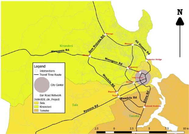
Dar es Salaam is a Mono Centric structure city; it has only one Central Business District (CBD) with the arterial roads originated from the residential area toward CBD and two ring roads, as shown in Fig. 1. This implies that social services and economic activities are located in the city center. Also, government and private offices, education institutions, supermarkets, financial institutions and Dar es Salaam port (import and export goods). Most of the commuters travel from the outskirts area of the city towards the CBD. This situation courses rapid and unpredictable traffic flow towards the CBD during peak hours. Traffic flows in one direction during the morning’s hours towards the city center and vice versa in the evening exceeds the capacity of the roads.
Fig. 1.
3.2. Data Collection and Analysis
The travel time data was collected in five main corridors which are:
• Mbagala-Kariakoo via Kilwa road; • Pugu - Kariakoo via Nyerere and Uhuru
roads;
• Mbezi - Kariakoo via Morogoro, Mandela and Uhuru roads;
• Tegeta - Kariakoo via Bagamoyo, Ali Hassan Mwinyi and United Nation road; • Kawe - Kariakoo via Old Bagamoyo and
Kawawa Roads.
These corridors were selected because the majority of commuters use them when making a trip to CBD and have a direct connection to the residential areas. Also, the corridors provide the link between the Dar es Salaam port authority and other parts of the country and outside of the countries. The travel time data were collected in three days a
week, which are Tuesdays, Wednesdays, and Thursdays. Mondays, Fridays and weekends were excluded in the sample because on Fridays, most of the road users move from the city to the outskirts area of the city for the weekend vacation and Mondays people who go for the weekend vacations return to their working places. Saturdays and Sundays most people stay at home for the weekend vacation; for that reason, traffic flow in the city is very low. The surveys conducted between October 2018 and January 2019 managed to collect data in twenty-eight 28 trips per day. This means that fourteen (14) trips per day per direction. Therefore, the general sample trips made are equal number trips made per Two Directions times Survey Days times Number of Corridors which is 420 trips, and the total number of links is similar to the sum of Total trips per day per corridor times Number of the Links per corridor which is 1344 trip links as indicated in Table 1.
Table 1
Surveyed Link and Duration
Corridor Name Survey Duration (hrs) No. of Trips Survey Days Total Trips No. of Links Total Trips
Tegeta -Kariakoo 14 28 3 84 5 420
Mbezi - Kariakoo 14 28 3 84 3 252
Pugu - Kariakoo 14 28 3 84 3 252
Mbagala - Kariakoo 14 28 3 84 2 168
Kawe - Kariakoo 14 28 3 84 3 252
Total 420 1344
The data were collected every one hour starting from 6.00 AM to 8.00 PM in these five main corridors. The data including travel time in each link, link distance, delay time at the intersections and waiting time of the bus at the bus stops as showing in Table 2. The public commuter buses (daladala)
Table 2
The Main Feature in the Five Corridors
Corridor Name Link Name Link Length (Km) No. of Bus Stops No. of Intersections
Tegeta - Kariakoo
Tegeta-Africana 5.5 8 2
Africana-Mwenge 7.2 9 4
Mwenge-Victoria 3.4 6 2
Victoria-Mbyuni 2.4 2 2
Mbuyuni-Kariakoo 6.7 7 5
Mbezi - Kariakoo
Mbezi-Ubungo 12.5 12 2
Ubungo-Buguruni 7.5 11 3
Buguruni-Kariakoo 3.6 7 2
Pugu - Kariakoo
Pugu-Aiport 11.3 15 1
Aiport-Buguruni 7.5 5 4
Buguruni-Kariakoo 3.6 8 2
Mbagala - Kariakoo Uhasibu-KariakooMbagala-uhasibu 7.05.0 1010 11
Kawe - Kariakoo
Kawe-Morocco 7.2 11 1
Morocco-Magomeni 3.8 6 4
Magomeni-Kariakoo 3.2 4 2
This study used secondary data, which were collected by JICA in collaboration with the NIT in 2017 and available in the National Institute of Transport (NIT) database.;a total of seventeen (17) points were surveyed, as indicated in Table 3. Some of the data were collected in 14 hours and others 24 hours.
Since the travel time survey was conducted from 6.00 AM to 8.00 PM, the data were merged. For example, for the case of a travel time survey when a trip was made from 6.00 AM-8.00 AM, the traffic flow data collected from 6.00 AM-8.00 AM was considered as the exact traffic flow at that time.
Table 3
Traffic Flow Data
Corridor Name Survey Time (hrs) Name of Points No. of Points
Tegeta - Kariakoo 14 and 24 Tegera,Makongo, Millenium ,Osterbay and Salender 5
Mbezi - Kariakoo 14 Mbezi (Mkaa), Kibo and Tabata sukita 3
Pugu - Kariakoo 14 Ukonga and Tazara 2
Mbaga - Kariakoo 14 Railway Bridge, Mvinjeni and Mbagala Mission 4
Kawe - Kariakoo 14 Mlalakua, Mkwajuni and Kigogo Sambusa 3
Total 17
Final data was edited and checked their reliability, whereby outliers and unusual travel time from the corridors were removed and adjusted. The data used to develop the models was normalized because the contribution of each input variable depends on the weight of
(1)
where, y is the normalized value, x is the targeted variable xmin and xmax are the
minimum and maximum variables.
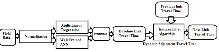
3.3. Travel Time Model Development
The model developed by incorporating the Multi-Linear Regression (MLR) and Artificial Neural Network (ANN) purposely to obtain a suitable baseline link travel time data. The field data includes link travel time, traffic flow, link distance, time of the day, intersections delay time and waiting time of the bus at
the bus stop; these data were used as input data into the MLR and ANN models. Both outputs from the Multi-linear Regression model and Artificial Neural Network were evaluated, compared in terms of R square, Root Mean Square Error (RMSE), and Mean Absolute Percentage Error (MAPE). The one which shows high performance in terms of less percentage error was considered as the suitable baseline link travel time data. These baseline-link travel time data was applied into the Kalman filter dynamic algorithm in collaboration with previous link travel time to obtain the dynamic travel time prediction model for the predict next link travel time as indicated in Fig. 2.
Fig. 2.
Travel Time Prediction Dynamic Framework
Kalman Filter algorithm was developed to adjust the baseline link travel time data from the MLR and ANN model in collaboration with previous link travel time shown in Fig. 2. The developed dynamic travel time prediction model can be used to predict travel time during inbound as well as outbound traffic directions. The field data applied MLR and ANN as follows.
3.3.1. Multi-Linear Regression Model
Multi-Linear Regression was applied using the data collected in five corridors in Dar es Salaam city. The independent variables used in the model are the waiting time of the bus
at the bus stop, delay time at the intersection, link distance, traffic volume, peak hours and off-peak hours. The dependent variable was the travel time in the links. The data used to build the regression analysis model were divided into two sets, 75 percent for training and 25 percent for testing. The Microsoft excel was used to analyze data to evaluate the multi-linear regression analysis model, as indicated in Eq. (2).
(2)
Where, TTsec is link travel time, X1 is traffic
and 0 for peak hours and off-peak hours, respectively. X2 is a bus waiting time at the bus
stops, X3 is a delay time at the intersections,
X4 is a link travel distance, X5 is traffic follow
volume in the five main corridors and a, b, c, d, e, and w are the constant parameters.
3.3.2. Artificial Neural Network and
Travel Time Prediction
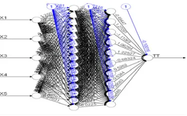
ANN has been applied in widely solving transportation problems because of its ability to deal with complex and nonlinear relationships between predictors that can arise from large amounts of data, specifically in predicting urban travel time (Bai et al., 2015). The ANN model uses the same input data collected in the field that used MLR model. ANN was applied to predict link travel time as shown in Fig. 3 and it consists of four (4) layers; one is the input layer with five (5) neurons, Two (2) hidden layers with 15, 10 neurons respectively and one output layer with one neuron. The input layer, hidden layers and output layer connected by networks (synapses), synapses carry the values which are known as weights. The input layer contains five variables, which are X1, X2, X3, X4, and X5, and the output layer
contains one dependent variable, which is TT. X1 is the traffic state data which was divided
into two groups, Peak Hours and off-peak, for
the peak hour was observed from 6.00 AM to 11.00 AM for inbound direction and 3.00 PM to 20.PM for outbound direction, while off-peak hours was observed from 11.00 AM to 8.00 PM for the inbound direction, 6.00 AM to 3.00 PM for the outbound direction. The XLSTAT software was used to simulate urban link travel time.
XLSTAT is the statistical analysis add-in that offers a wide variety of functions to enhance analytical capabilities. It is compatible with all Excel versions, such as Microsoft version 2003 to version 2016 (2011 and 2016 for Mac). XLSTAT-R options tools with a neural net dialog box, where travel time for the five corridors was inserted as a dependent variable, while five variables X1, X2, X3, X4, and
X5 were inserted as independent variables.
The activation function was introduced as a nonlinear relationship between the input layer and the output layer. The sigmoidal function, such as logistic and tangent hyperbolic is common because of its ability to normalize the input values to the range of -1 to 1. Most of the studies dealing with urban traffic prediction prefer to use logistic and tangent hyperbolic because they produce positive and negative value and are faster in training (Fan and Gurmu 2015; Amita et al., 2016; Čelan and Lep, 2017; Zhu et al., 2018).
Fig. 3.
In this training processes XLSTAT (neural net toolbox) was set as follow Neurons per hidden layers: 15, 10, Threshold: 0.01, Maximum steps: 100000, Repetitions: 1, type of algorithm: (Resilient backpropagation) RProp+ , Error function: Squared errors, Activation function: Logistic. Validation and testing of the neural network are essential to justify the training accuracy if it is sufficient. Therefore, the sample data were divided into two sets, one set was used to training the travel time model and another set was used to validate the model during the model development. However, there is no general producer for the portion of the sample data, but several factors should be considered during the division of the data, such as type of the data and sample size. The final cleaned data were divided into 75 percent of data for training and 25 percent of the data for testing the model. This has been adopted by many researchers (Jiang
et al., 2014; Bai et al., 2015; Fan and Gurmu, 2015). During the training and learning process weights and biases were adjusted automatically in the hidden layers (Amita et al., 2015). The output from the MLR and ANN may not be used directly to predict the next link travel time because the MLR and ANN models were built by using historical data. Kalman Filter algorithm will be applied to adjust output of MLR or ANN. After been compared
3.3.3. Kalman Filter Algorithm
Kalman filtering is an algorithm that provides a prediction of some unknown variables given the current measurement and previous estimate over time. The output from MLR or ANN used as a current measure, later on, were adjusted by the Kalman filter algorithm to the net link travel time. The output from the ANN or MLR was used as baseline data for predicting the next link travel time. Kalman filter was used to
estimate states based on linear dynamical systems in state-space format. The process model defines the evolution of the state from time k - 1 to time k as indicated in Eq. (3).
(3)
where F is a state transition vector applied in the previous state vector Xk-1 B is the control
input vector applied in the previous control vector Uk-1 and Wk-1 is the process noise which
assumed to be zero mean and Gaussian with covariance Q.
The process was paired with the measured model that describes the relationship between that state and measurement at the current time step k as indicated in Eq. (4).
(4)
where, Zkis the measurement vector, H
is the measurement matrix, and Vk is the
measurement noise vector that is assumed to be zero-mean Gaussian with the covariance R.
The role of Kalman Filter is to provide the estimate of Xk at time k, given the initial
estimate of Xo, the series measurement Z1, Z2,
Z3………Zk and the information of the system
described by F, B, H, Q , and R.
It is known that the covariance matrices are supposed to reflect the statistics of the noises; the actual statistics of the noises are not known or not Gaussian in many practical applications’ initial stage. Therefore, Q and R
are usually used as tuning parameters that the user can adjust to get the desired performance.
Table4
Kalman Filter Dynamic Algorithm
Prediction
Predicted State Estimate Xk =FXk−1+BUk−1
Extrapolation Error Covariance Pk−=FPk−1+FT+Q
Update
Measure Residual yk =zk−Hxk
Kalman Gain
T k
k T
k P H K
R HP H
= +
Update Estimate Xk =Xk−1+K Yk k
Update Error Covariance Pk = −(1 K Pk) k−
4. Results and Discussions
4.1. Travel Time Variations
The data were analyzed and computed, as shown in Table 5, in which it is observed that travel time has almost similar descriptive statistics such as mean and Standard
Deviation. It has been observed that the average travel time for the four main corridors for three days ranged from 20.8 to 22.0 minutes for inbound direction and 21.0 to 21.9 minutes for outbound direction. Travel time varies from 8.9 to 9.1 minutes for inbound direction 8.2 and 8.6 minutes for outbound direction.
Table 5
Sample Size of Each Route and Descriptive Statistics
Day Average (Min) STDEV (Min.)
Inbound Outbound Inbound Outbound
Tuesday 21.6 21.0 9.0 8.2
Wednesday 20.8 21.9 9.1 8.5
Thursday 22.0 21.9 8.9 8.6
Figures 4 and 5 represent travel time in each link for three days (Tuesdays, Wednesdays and Thursdays) for inbound and outbound directions, respectively. Travel time prediction has an association with level of uncertainty, which depends upon underlying variability of the data as well as sample. Travel time variations for each link were a significant factor as it shows
Fig. 4.
Travel Time Variation Inbound Directions
Fig. 5.
Travel Time Variation Outbound Directions
4.2. Model Performance and Evolution
4.2.1. Comparison of MLR and ANN models
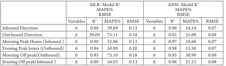
MLR and ANN models were applied to evaluate their prediction accuracy based on R squared, Mean Absolute Percentage and Root Mean Square. Their performance evaluation as indicated in Table 6
Table 6
Comparison between MLR and ANN Models
MLR- Model R2
MAPE% RMSE
ANN- Model R2
MAPE% RMSE
Variables R2 MAPE% RMSE Variables R2 MAPE% RMSE
Inbound Direction 6 0.88 39.69 0.13 6 0.96 18.54 0.07
Out bound Direction 6 39.69 75.11 0.18 6 0.82 25.69 0.08
Morning Peak Hours (Inbound ) 6 0.90 32.86 0.13 6 0.97 18.68 0.07
Evening Peak hours (Outbound) 6 0.84 50.89 0.20 6 0.98 15.50 0.07
Morning Off peak(Outbound) 6 0.85 75.10 0.18 6 0.95 30.99 0.09
From Table 6, it can be observed that the MLR model has higher MAPE and RMSE values compared to ANN model this indicates that it has poor performance. Whereas, the ANN model has high R square values compared to MLR model, which is good performance compared to MLR model. Therefore, the ANN model was considered as the suitable model. This suitable model will be compared withANN-Kalman Filter (ANN-KF) model.
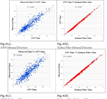
4.3. Comparison of ANN and
ANN-Kalman Filter (ANN-KF) Models
After developing ANN-KF model it was necessary to evaluate its performance in
terms of prediction accuracy. The prediction accuracy evaluated and compared with ANN model employing R2.
From Fig. 6 (a, b, c and d), the values of R square for ANN model range from 82 to 84 percent, which indicate that more than 82 percent of field data were presented by the ANN model.
Furthermore, about 99 percent of predicted travel time from ANN-KF model was represented by predicted travel time from ANN model, which implies that 99 percent of the predicted travel time by ANN-KF model was well fitted in the ANN model.
Fig. 6(a) . Fig. 6(b).
ANN Inbound Direction Kalma Filter Inbound Direction
Fig. 6(c). Fig. 6(d).
4.4. Model Evaluation
The evaluation of ANN-KF model was done based on Root Mean Square Error (RMSE) and Mean Absolute Percentage Error (MAPE) to measure the accuracy of the travel time model.
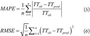
The calculation of the error value and percent error to determine model deviation from the actual travel time predicted by the ANN model and predicted ANN-KF model was done using the following relationships Eq. (5) and Eq. (6):
1
1 n
ob pred
i ob
TT TT
MAPE
n = TT
−
=
∑
(5)(
)
21
1 n
ob pred
i
RMSE TT TT
n =
=
∑
− (6)Where TTob is predicted travel time from
ANN, TTpred , is predicted bus travel time
from ANN-KF model and n is number of bus trips observed in the main corridors. In this study the model performance were evaluated as whole travel time in four main corridors based on the inbound and outbound direction as shown in Table 7.
Table 7
Comparison of Prediction Errors for Two Models
ANN - Model ANN-KF Model
MAPE% RMSE MAPE% RMSE
Inbound Direction 18.54 0.07 8.72 0.02
Out bound Direction 25.69 0.08 10.58 0.20
Morning Peak Hours (Inbound ) 18.68 0.07 6.11 0.21
Evening Peak hours (Outbound) 15.50 0.07 5.24 0.22
Morning Off peak(Outbound) 30.99 0.09 8.63 0.23
Evening Off peak(Inbound ) 21.23 0.08 7.14 0.02
The results in table 7 showed that the average deviation between the observed and the predicted travel time in the ANN model was between 18.54 and 25.69.percent, while for ANN-KF model was between 8.72 and 10.58 percent from ANN model in both directions. Therefore, the integration of the Artificial Neural Network and Kalman Filter algorithm model promised to be a reasonable model for predicting dynamic travel time in Dar es Salaam city.
5. Conclusion and Recommendation
The study developed and introduced the use of ANN - KF model for predicting travel time
in heterogeneous traffic flow conditions in the developing countries. This model is a result of integration of ANN model and Kalman Filter dynamic algorithm, whereby this approach is used to capture the uncertainties of urban travel time. The ANN model produces the suitable baseline data after being compared with MLR through use R2 ,MAPE, and
The overall results indicate that ANN-KF model has minimum error and hence can be applied in heterogeneous traffic condition to predict travel time.
The travel time prediction model employed six variables and five corridors to predict travel time for commuters to raise awareness of mode of transport and selected route purposely to minimize travel time, this model can be applied in developing countries. However, due to the rapid growth of urbanization and economic activities in developing countries particularly in Tanzania, the ANN-KF model may need to be calibrated. This model can be extended by expanding coverage area and incorporating other variables like driving behaviors, weather conditions, and other incidents like accidents.
Acknowledgment
The authors would like to acknowledge the support given by the National Institute of Transport and JICA for providing data used in this study
References
Amita, J.; Singh, J.S.; Kumar, G.P. 2015. Bus Travel Time Using Artificial Neural Network, International Journal for Traffic and Transport Engineering 5(4): 410-424. Amita, J.; Jain, S.S.; Garg, P.K. 2016. Prediction of Bus Travel Time using ANN: A Case Study in Delhi,
Transportation Research Procedia 17: 263-272.
Arhin, S.; Noel, E.; Anderson, M.F.; Williams, L.; Ribisso, A.; Stinson, R. 2016. Optimization of transit total bus stop time models, Journal of Traffic and transportation Engineering 3(2): 146-153.
Bai, C.; Peng, Z.R.; Lu, Q.C.; Sun, J. 2015. Dynamic Bus Travel Time Prediction Models on Road with Multiple Bus Routes, Computational Intelligence and Neuroscience
2015(432389): 1-9.
Chen, M.; Liu, X.; Xia, J.; Chien, S.I. 2004. A Dynamic Bus‐Arrival Time Prediction Model Based on APC Data, Computer‐Aided Civil and Infrastructure Engineering
19(5): 364-376.
Chien, S.I.J.; Kuchipudi, C.M. 2003. Dynamic Travel Time Prediction with Real-Time and Historic Data,
Journal of Transportation Engineering 129(6): 608-616. Chien, S.I.J.; Ding, Y.; Wei, C. 2002. Dynamic Bus Arrival Time Prediction with Artificial Neural Networks, Journal of Transportation Engineering 128(5): 429-438.
Čelan, M.; Lep, M. 2017. Bus Arrival Time Prediction Based on Network Model, Procedia Computer Science
113: 138-145.
Elhenawy, M.; Chen, H.; Rakha, H.A. 2014. Dynamic Travel Time Prediction Using Data Clustering and Genetic Programming, Transportation Research Part C: Emerging Technologies 42: 82-98.
Fan, W.; Gurmu, Z. 2015. Dynamic Travel Time Prediction Models for Buses Using Only GPS Data,
International Journal of Transportation Science and Technology
4(4): 353-366.
Jeong, R.; Rilett, R. 2004. Bus Arrival Time Prediction Using Artificial Neural Network Model. In Proceedings of the 7th International IEEE Conference on Intelligent Transportation Systems, 988-993.
Jindal, I.; Qin, T.; Chen, X.; Nokleby, M.; Ye, J. 2017. A Unified Neural Network Approach for Estimating Travel Time and Distance for a Taxi Trip. Available from internet: <http:// http://arxiv.org/abs/1710.04350>. Kumar, B.A.; Vanajakshi, L.; Subramanian, C. 2014.
Pattern-Based Bus Travel Time Prediction under Heterogeneous
Traffic Conditions. Transportation Research Record,
Transportation Research Board, National Research Council, Washington, DC. 16 p.
Kumar, B.A.; Vanajakshi, L.; Subramanian, S.C. 2018. A hybrid model based method for bus travel time estimation, Journal of Intelligent Transportation Systems
22(5): 390-406.
Kumar, B.A.; Vanajakshi, L.; Subramanian, S.C. 2017. Bus Travel Time Prediction Using a Time-Space Discretization Approach, Transportation Research Part
C: Emerging Technologies 79: 308-332.
Li, M.; Wu, H.; Wang, Y.; Handroos, H.; Carbone, G. 2017. Modified Levenberg–Marquardt Algorithm for Backpropagation Neural Network Training in Dynamic Model Identification of Mechanical Systems, Journal
of Dynamic Systems, Measurement, and Control 139(3):
031012. 14 p.
Shi, C.; Chen, B.; Li, Q. 2017. Estimation of Travel Time Distributions in Urban Road Networks Using Low-Frequency Floating Car Data, ISPRS International Journal of Geo-Information 6(8): 253.
Wu, C.H.; Ho, J.M.; Lee, D.T. 2004. Travel-Time Prediction with Support Vector Regression, IEEE transactions on intelligent transportation systems 5(4): 276-281.
Xiong, G., Kang, W., Wang, F., Riekki, J., & Pirttikangas, S. (2015). Continuous Travel Time Prediction for Transit Signal Priority Based on a Deep Network. IEEE 18th International Conference on Intelligent Transportation Systems
Continuous 92: 523-528.
Yu, Z.; Wood, J.S.; Gayah, V.V. 2017. Using Survival Models to Estimate Bus Travel Times and Associated Uncertainties, Transportation Research Part C: Emerging Technologies 74: 366-382.
Zaki, M.; Ashour, I.; Zorkany, M.; Hesham, B. 2013. Online Bus Arrival Time Prediction Using Hybrid Neural Network and Kalman Filter Techniques,
International Journal of Modern Engineering Research 3(4): 2035-2041.
Zheng, F. 2011. Modeling Urban Travel Times. Thesis Series T2011/9, The Netherlands TRAIL Research School. Zheng, F.; Van Zuylen, H. 2013. Urban Link Travel Time Estimation Based on Sparse Probe Vehicle Data,
Transportation Research Part C: Emerging Technologies 31: 145-157.