www.nat-hazards-earth-syst-sci.net/13/2353/2013/ doi:10.5194/nhess-13-2353-2013
© Author(s) 2013. CC Attribution 3.0 License.
Natural Hazards
and Earth System
Sciences
Integrating spatial, temporal, and size probabilities for the annual
landslide hazard maps in the Shihmen watershed, Taiwan
C. Y. Wu and S. C. Chen
Department of Soil and Water Conservation, National Chung-Hsing University, Taichung 40227, Taiwan Correspondence to: S. C. Chen (scchen@nchu.edu.tw)
Received: 23 February 2013 – Published in Nat. Hazards Earth Syst. Sci. Discuss.: 19 March 2013 Revised: 13 August 2013 – Accepted: 13 August 2013 – Published: 25 September 2013
Abstract. Landslide spatial, temporal, and size probabilities were used to perform a landslide hazard assessment in this study. Eleven intrinsic geomorphological, and two extrinsic rainfall factors were evaluated as landslide susceptibility re-lated factors as they rere-lated to the success rate curves, land-slide ratio plots, frequency distributions of landland-slide and non-landslide groups, as well as probability–probability plots. Data on landslides caused by Typhoon Aere in the Shihmen watershed were selected to train the susceptibility model. The landslide area probability, based on the power law re-lationship between the landslide area and a noncumulative number, was analyzed using the Pearson type 5 probabil-ity densprobabil-ity function. The exceedance probabilities of rainfall with various recurrence intervals, including 2, 5, 10, 20, 50, 100 and 200 yr, were used to determine the temporal proba-bilities of the events. The study was conducted in the Shih-men watershed, which has an area of 760 km2and is one of the main water sources for northern Taiwan. The validation result of Typhoon Krosa demonstrated that this landslide haz-ard model could be used to predict the landslide probabilities. The results suggested that integration of spatial, area, and exceedance probabilities to estimate the annual probability of each slope unit is feasible. The advantage of this annual landslide probability model lies in its ability to estimate the annual landslide risk, instead of a scenario-based risk.
1 Introduction
Taiwan is often affected by landslides because of its steep to-pography, fragile geology, seismic activity, and rapid devel-opment in the mountainous regions. After the Chichi earth-quake (ML=7.3 in 1999), the affected areas became more
susceptible to landslides, and heavy rainfall during typhoons or storms have indeed caused large landslides of loosened soil (Wu and Chen, 2009). Furthermore, climate change en-larges bare land areas, thereby increasing the frequency of landslides in Taiwan (Chen and Huang, 2010). Because of the uncertainties associated with natural disasters, risk man-agement is necessary to minimize losses (Chen et al., 2010). In view of the growing emphasis on risk management in dis-aster prevention work, quantitative assessment of landslide risk is becoming increasingly important. In particular, the landslide hazard analysis is the most important step in risk assessment. Therefore, a landslide hazard model that can be used as a basis for landslide risk analysis was established in this study.
The accepted definition of landslide hazard was proposed by Varnes and IAEG (1984). Guzzetti et al. (1999) incorpo-rated “magnitude of event” into this definition to redefine landslide hazard. Further, Guzzetti et al. (2005) established a landslide hazard probability model. Thus, landslide spatial probability, landslide temporal probability, and landslide size probability were combined to construct the landslide hazard probability model in this study.
Landslide spatial probability is also known as landslide susceptibility, which can be estimated using qualitative or quantitative methods. Quantitative statistical analysis meth-ods included bivariate analyses (Chung and Fabbri, 1993; Zêzere et al., 2007), multivariate regression (Carrara, 1983; Baeza and Corominas, 2001), logistic regression (Lee et al., 2008; Rossi et al., 2010; Nefeslioglu and Gokceoglu, 2011), and discriminant analysis (Guzzetti et al., 2006; Carrara et al., 2008).
probability model has been used to estimate the temporal recurrence probability in studies, including flooding proba-bility research (Onoz and Bayazit, 2001) and landslide prob-ability research (Guzzetti et al., 2005; Ghosh et al., 2012b). However, because the data on natural hazards rely on limited time periods, it was necessary to develop flexible methods to avoid inconsistencies that exist between the assumptions of the Poisson probability model (Crovelli, 2000) and the real situation. For example, rainfall factors can be considered im-portant triggering factors for landslide and debris flow haz-ards, because rainfall intensity in different return periods lead to different scale of landslide and debris flow hazards. Using the exceedance probability of various rainfall return periods to estimate the probability of landslide and debris flow events can also achieve the goal of estimating temporal probability to a certain degree (Bründl et al., 2009; Chen et al., 2010).
On the probability of landslide size, Bak et al. (1988) argued that self-organized criticality (SOC) occurs in nat-ural landslides. Malamud et al. (2004) verified the power law relationship between landslide area and noncumulative frequency. They also fit the probability density function of a landslide area with common functions, and found good agreement with a truncated inverse gamma distribution. In addition, Stark and Hovius (2001) achieved a good agree-ment after conducting a double Pareto distribution to fit a probability density function of the landslide area.
The purpose of this study was to establish a landslide haz-ard model that can be used to estimate the annual landslide probability. The landslide spatial, temporal, and size proba-bilities were analyzed based on the landslide inventory from 1996 to 2009, 13 variables of landslide susceptibility factors, and rainfall data of those events in the Shihmen watershed. This watershed covers an area of 760 km2, and is one of the main water sources for northern Taiwan. The Shihmen watershed was divided into 9181 slope units, and the the-matic variables of individual slope units were then derived, screened, and entered in the logistic regression analysis. Data of landslides caused by Typhoon Aere were selected to train the susceptibility model. The landslide area probability was analyzed using the Pearson type 5 probability density func-tion, based on all the new landslides that occurred from 1996 to 2009. The exceedance probabilities of rainfall with vari-ous recurrence intervals, including 2, 5, 10, 20, 50, 100 and 200 yr, were used to determine the temporal probabilities of the events. The spatial, area, and exceedance probabilities were integrated to estimate the annual landslide probability of each slope unit in the Shihmen watershed. The feasibility of the integration of this annual landslide probability model was verified by comparing the results with the results of the Poisson landslide probability model for each slope unit. The results indicated that the landslide probability model estab-lished for this study can be used for landslide risk analysis. The annual risk, rather than a scenario-based risk, can be es-timated using this model.
27 1
2
Fig. 1. The river system, roads, and topography of the Shihmen watershed. The landslides 3
were caused by Typhoon Aere in 2004. 4
5
Fig. 1. The river system, roads, and topography of the Shihmen watershed. The landslides were caused by Typhoon Aere in 2004.
2 Data acquisition and processing
2.1 Environmental setting of the Shihmen watershed
The Shihmen watershed straddles Taoyuan, Hsinchu, and Yi-lan counties, and the reservoir is mainly fed by the Dahan River. This watershed has an area of approximately 760 km2, and the Shihmen Reservoir is the third largest reservoir in Taiwan and one of the main water sources for northern Tai-wan. The geographical extent and river system of the wa-tershed are illustrated in Fig. 1. The area is mountainous, and is higher in the south than in the north. The elevation ranges from 236 to 3527 m, with an average elevation of approximately 1409 m. The average slope is approximately 34◦, and the slope decreases progressively from the
south-east to the northwest. With regard to the regional geology, outcrops in the area primarily consist of the Oligocene Bal-ing stratum, which occupies approximately 35.07 % of the total area, Eocene Siling sandstone, which occupies approx-imately 16.20 % of the area, and the Miocene Wenshui stra-tum, which occupies 12.43 % of the area. As far as land use is concerned, most land within the area consists of undeveloped
1
2
Fig. 2. The temporal pattern of rainfall recorded at the New Baishi station during Typhoon
3
Aere.
4
5
Fig. 2. The temporal pattern of rainfall recorded at the New Baishi station during Typhoon Aere.
forest, which occupies 92.44 % of the total area, followed by farmland, which occupies 2.71 % of the overall area. 2.2 The landslide inventory in the Shihmen watershed
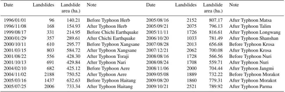
The landslide inventory for the Shihmen watershed covered the 1996–2009 temporal interval (Table 1). New and expan-sive landslides caused by Typhoon Aere in 2004 occupied 579 ha, or 77 % of the total landslide area. Therefore, this event was selected as the research subject. Numerous land-slides were found in the watershed, especially in the up-stream basin of the Baishi River (Fig. 1).
2.3 The available data of landslide susceptibility factors
The lithology, slope, aspect, elevation, normalized differen-tial vegetation index (NDVI), terrain roughness, slope rough-ness, total slope height, distance from road, distance from fault, and distance from river were preliminarily selected as intrinsic causative factors in this study. Lithology was chiefly classified as argillite, quartzitic sandstone, hard sandstone and shale, sandstone and shale, terrace deposits, and allu-vium on the basis of the 1:50 000 geologic maps from the Central Geological Survey.
Slope, aspect, and elevation data were acquired from a dig-ital elevation model (DEM), using the ArcGIS program. The 5 m×5 m DEM generated from aerial photographs was used in this analysis. Terrain roughness and slope roughness (Wil-son and Gallant, 2000) are usually determined using a type of neighborhood analysis, such as an analysis within a 5-cells moving window (Cavalli et al., 2008), to establish the rough-ness value for each grid. However, in this study, the terrain variability of the entire slope unit, rather than the variability of local parts in the slope unit, was considered. The stan-dard deviation of the elevation calculated by the elevations of the entire grid within each slope unit was used to indicate the terrain roughness. The slope roughness was simultane-ously selected in this study according to the effectiveness in other researches (Lee et al., 2008; Chen et al., 2013). Simi-larly, the standard deviation of the slope in each slope unit was calculated to express the slope variability, which was then used to indicate the slope roughness. In addition, the height differential from the crest to the toe of the slope in each slope unit was used to indicate the total slope height. The total slope height may be physically related to the mag-nitude of the stress and the pore-water pressure in the lower slope, and for long slopes the surface and subsurface water is more likely to be concentrated in the lower slope, which causes instability (Lee et al., 2008).
NDVI values were determined by taking advantage of the absorption of red light and reflection of near-infrared light emitted by green plants. The NDVI values, which ranged from−1 to 1, were calculated from SPOT images taken be-fore Typhoon Aere. The horizontal distance of each slope unit from roads, faults, or perennial rivers were used to reflect the effect of roads, faults, and rivers on landslides. The loca-tions of all the faults (Fig. 1) were extracted from 1:50 000 geologic maps published by the Central Geological Survey, and the locations of all the perennial rivers were extracted from 1:5000 orthophoto base maps of Taiwan published by the Aerial Survey Office, Forestry Bureau.
Table 1. The multi-year landslide inventory of the Shihmen watershed.
Date Landslides Landslide Note Date Landslides Landslide Note
area (ha.) area (ha.)
1996/01/01 96 140.21 Before Typhoon Herb 2005/08/16 2152 807.17 After Typhoon Matsa 1996/11/08 168 154.93 After Typhoon Herb 2005/09/21 2075 796.13 After Typhoon Talim 1999/08/17 331 214.95 Before Chichi Earthquake 2005/11/11 1726 816.61 After Typhoon Longwang 2000/01/29 357 289.61 After Chichi Earthquake 2006/10/20 1033 781.49 After Typhoon Shanshan 2000/10/11 610 295.77 Before Typhoon Xangsane 2007/08/28 2013 656.68 Before Typhoon Krosa 2001/03/15 803 584.72 After Typhoon Xangsane 2007/12/21 2062 700.08 After Typhoon Krosa 2001/08/22 556 428.30 After Typhoon Toraji 2008/08/16 1728 566.56 Before Typhoon Nuri 2001/10/13 691 429.84 After Typhoon Nari 2008/08/24 1708 559.71 After Typhoon Nuri 2004/02/10 682 425.12 Before Typhoon Aere 2008/11/06 2000 704.44 After Typhoon Jangmi 2004/11/02 2188 750.52 After Typhoon Aere 2009/05/08 1889 732.22 Before Typhoon Morakot 2005/03/16 1437 632.63 Before Typhoon Haitang 2009/08/20 1860 779.31 After Typhoon Morakot 2005/07/25 2006 733.34 After Typhoon Haitang 2009/10/21 2521 789.92 After Typhoon Parma
occurred from 18:00 on 24 August to 06:00 on 25 August, and the cumulative rainfall reached 1600 mm. The maximum cumulative rainfalls of various durations were also analyzed. The maximum 12 h cumulative rainfall was 842 mm, approx-imately 52 % of the total rainfall, and the maximum 24 h cu-mulative rainfall was 1262 mm, approximately 78 % of the total rainfall.
3 Methodology
Landslide hazard is defined as the probability of occurrence within a specified period of time and within a given area of a landslide event with a certain magnitude (Guzzetti et al., 2005; Ghosh et al., 2012a). Therefore, the landslide haz-ard probability, (HL), within a given area can be obtained from the conditional probability of landslide spatial probabil-ity,P (SL), of the temporal probability of a landslide event,
P (NL), and of the landslide size probability P (AL). The
HLcan be calculated based on the independence assumption among the three probabilities using the following equation:
HL=P (SL)×P (NL)×P (AL). (1)
Landslide inventory maps, thematic variables of land-slide susceptibility factors, and rainfall data of landland-slide events were used for the landslide hazard analysis, which included landslide susceptibility (spatial probability), occur-rence probability of the landslide event (temporal probabil-ity), and landslide size probability. In this study, rainfall was chosen as the sole triggering factor because most landslides included in the inventory maps had been caused by typhoons or torrential rains.
3.1 Landslide spatial probability distribution
The watershed was divided into several slope units, and the thematic variables of each individual slope unit were sub-sequently derived, screened, and entered in the logistic re-gression to perform the landslide susceptibility analysis. The
landslide spatial probability was obtained after testing and validating the model.
Over 50 types of landslide thematic variables have been considered or used in related studies (Lin, 2003). Based on the references, the following factors were preliminarily se-lected as the intrinsic causative factors in this study: lithol-ogy, slope, aspect, elevation, normalized differential vegeta-tion index (NDVI), terrain roughness, slope roughness, total slope height, distance from road, distance from fault, and dis-tance from river. Various rainfall-related data were used as extrinsic triggering factors. The landslide thematic variables were selected as effective variables using a success rate curve (SRC), landslide ratio plot, frequency distribution of land-slide and non-landland-slide group, and probability–probability plot (P–P plot) for each variable based on the quantitative landslide thematic variable screening procedures of the Cen-tral Geological Survey (2009).
Because the area under the curve (AUC) can be used to determine the effectiveness of a model (Chung and Fabbri, 1999), the SRCs were used to determine the ability of the model to explain training data. The AUC value can range from 0 to 1, and the closer the value is to 1, the more per-suasive the result. The AUC value of the SRC was used to assess the ability of the thematic variables to predict land-slides. After calculating the ratio of landslide sample num-bers to the total number of slope units in each value interval for each variable, landslide ratio plots demonstrating the re-lationship between landslide ratios and the various value in-tervals were drawn to determine whether the landslide trends were consistent with the physical meanings of the variables. The goal of these frequency distribution plots was to deter-mine whether the frequency distribution of both the landslide and non-landslide groups could be differentiated, and hence whether the variable could be used to distinguish the land-slide from the non-landland-slide group. A P–P plot was used to inspect the relationship between a certain variable and a spe-cific distribution.
After establishing the landslide susceptibility model and calculating the landslide susceptibility index for each slope unit, the model accuracy was assessed using a classification error matrix, SRC, and the frequency distribution of the land-slide and non-landland-slide groups. Subsequently, the slope units were ranked with high susceptibility, medium susceptibility, and low susceptibility grades on the basis of their susceptibil-ity indices, and thus enabled the drawing of the landslide sus-ceptibility maps. However, the level of sussus-ceptibility index (0−1) could not be directly treated as the landslide spatial probability. The spatial probability in this study was there-fore determined using the relationship between the landslide ratio and landslide susceptibility index. The landslide ratio was the ratio of the landslide sample numbers to the number of slope units for each susceptibility index interval (Lee et al., 2008). The ratios represented the landslide spatial probabil-ities for the slope units with different susceptibility indices. The slope units that belonged to the same susceptibility in-dex interval would have the same landslide spatial probabil-ity. This was achieved by calculating the landslide ratio for each susceptibility index interval, then plotting the relation-ship between the landslide ratio and the various value inter-vals, and converting the various susceptibility indices to spa-tial probabilities. Relationship plots were also used to verify whether the actual landslide trends were consistent with the degrees of landslide susceptibility.
3.2 Temporal probability of landslides
Any of two method categories could be selected to analyze the landslide temporal probability, based on the number of years of landslide data. The first category consisted of land-slide data before and after a single landland-slide event alone. The hourly rainfall data were collected from rain gauge stations in the study area during a typhoon or torrential rain that trig-gered landslides. Frequency analysis of the rainfall data was used to derive the exceedance probability of each relevant rainfall event, and thus to obtain the temporal probability of event-based landslides.
The second category consisted of a multi-year landslide inventory. In this case, the Poisson probability model was used to calculate the recurrence intervals of historical land-slide events and the temporal probability of landland-slides based on the assumptions (Crovelli, 2000). The Poisson probability model of experiencingnlandslides during timetis given by the following equation:
P[N (t )=n] =exp(−λt )×(λt )n/n!, (2)
whereλis the mean occurrence probability of landslides, and its reciprocalµis the mean recurrence interval between land-slides in years. The probability that one or more landland-slides will occur during timetis given by the following equation:
P[N (t )=1] =1−P[N (t )=0] =1−exp(−t /µ). (3)
3.3 Landslide size analysis
Bak et al. (1988) derived the distribution of landslide area and landslide noncumulative number, and found that the number of landslides increases with the landslide area up to the highest value; then it decays following a power law:
NL=C0A
−β
L , (4)
whereALis the landslide area,NLis the noncumulative num-ber of that landslide area, andβ andC0are constants.
Numerous studies have verified the power law relationship between landside area and noncumulative frequency, includ-ing studies of rainfall-induced landslides (Fujii, 1969; Hov-ius et al., 2000; Weng, 2009; Jaiswal et al., 2011; Ghosh et al., 2012b) and earthquake-induced landslides (Guzzetti et al., 2002).
The probability density function of the landslide area was fitted with a Pearson type 5 distribution (i.e., inverse gamma distribution). After ranking the landslide area from small to large, various parameters of this distribution function (esti-mated by fitting) were used to calculate the corresponding cumulative probability of various landslide areas. Thus, the probability of one specific landslide area could be predicted when a landslide occurred in the slope units.
4 Results of landslide probabilities
4.1 Variable selection of the susceptibility model
Slope units have more geomorphological and geological sig-nificance than grid units because of their relatively unbroken geomorphological boundaries. The slope units were conse-quently employed as the basic units of analysis in this study. Guided by the division method used by Xie et al. (2004), the GIS-based hydrologic analysis and modeling tool, Arc Hydro (David, 2002), was used to divide the watershed into slope units. The smallest slope units had areas larger than the average landslide area (Van Den Eeckhaut et al., 2009), which reduced the chance that a single landslide would be divided among various slope units, ensuring relatively opti-mal analytical results. Additionally, the DEM (5 m) of the Shihmen watershed was used to divide the watershed into slope units. The original topography could be divided into 659 sub-watersheds, and the combination of sub-watershed units before and after reversal yielded the slope units. A total of 9181 slope units were obtained, and the average size of a slope unit was approximately 8.28 ha.
29
Terrain roughness Average NDVI Average elevation
SRCs
LRDs
FD
s
P-P plots
1
Fig. 3. Success rate curves (SRCs), landslide ratio distributions (LRDs), frequency 2
distributions of landslide and non-landslide group (FDs), and probability-probability plots (P-3
P plots) of representative variables. 4
Fig. 3. Success rate curves (SRCs), landslide ratio distributions (LRDs), frequency distributions of landslide and non-landslide group (FDs), and probability-probability plots (P–P plots) of representative variables.
and average elevation were variables that were excluded in the first and second step of the screening, respectively. Fur-thermore, in the frequency distribution of the landslide and non-landslide group, the discriminantDj was also used to judge the variables’ ability to distinguish between the land-slide and non-landland-slide groups. InDj = Aj−Bj Sj, Aj was the mean value for the landslide group,Bjwas the mean
value for the non-landslide group, and Sj was the pooled standard deviation for the two groups. The AUC value and
Djfor each variable are demonstrated in Table 2.
With regard to the selection standard used in variable se-lection, the first step was to check whether the AUC value was greater than 0.5, and if it was less than 0.5, the factor was considered a random variable in the model, and was assumed
Table 2. The AUC value andDjfor each variable.
Variable AUC Dj Variable AUC Dj
Maximum slope 0.678 0.736 Average aspect 0.526 −0.114 Average slope 0.629 0.526 Average NDVI 0.481 0.087 Slope roughness 0.603 0.398 Minimum NDVI 0.651 −0.650 Highest elevation 0.527 0.155 Distance from fault 0.521 −0.117 Average elevation 0.506 0.050 Distance from road 0.512 −0.062 Total slope height 0.683 0.779 Distance from river 0.609 −0.556 Terrain roughness 0.685 0.789 Lithology 0.523 −0.136
to increase the model error (Dahal et al., 2008). Furthermore, the landslide ratio plot had to be consistent with the phys-ical meaning of each variable. For instance, the greater the distance from road, the smaller the landslide ratio was. The analysis results indicated that the variable eliminated in the first step was average NDVI. In the second step, the absolute value of the discriminantDj had to exceed 0.1 (aDj value greater than 0 indicated that the mean value of the landslide group was relatively large, and a value less than 0 indicated that the non-landslide group had a larger mean value), or the P–P plot indicated that the values had a normal distribution. Based on the analysis results, the average elevation and dis-tance from road were eliminated in the second step. Finally, maximum slope, average slope, slope roughness, highest el-evation, total slope height, terrain roughness, average aspect, minimum NDVI, distance from fault, distance from river, and lithology were selected as intrinsic thematic factors.
The extrinsic triggering variables were selected after cal-culating the maximum 1, 2, 3, 6, 12, 24, 48, 72, as well as 96 h rainfall at each rain gauge station during Typhoon Aere, and estimating the rainfall distribution throughout the entire research area by the geostatistical method. Ordinary krig-ing was first used in the geostatistical analysis. Cokrigkrig-ing was also used in analyses with rainfall as the primary vari-able, and elevation as a secondary variable. In addition, an-other cokriging method was used with rainfall as the primary variable and elevation, slope, and aspect as secondary vari-ables. Spherical and Gaussian models were chosen as semi-variogram models in the analyses using these three methods, and therefore yielded six combinations.
Several indicators of prediction error were inspected to compare the various models. A model complying with the following conditions was considered optimal: a mean value close to 0; a mean standardized value close to 0; the small-est root mean square; the average standard error clossmall-est to the root mean square; and the root-mean-square standardized value closest to 1. In addition, the rainfall distribution esti-mated using the geostatistical methods was compared with the distribution of landslides triggered by Typhoon Aere. Then, SRCs of various rainfall distributions were drawn to calculate the AUC values.
The results of this comparison indicated that the maximum 1 h rainfall (cokriging with Gaussian semivariogram model and elevation variable), and the maximum 24 h rainfall (ordi-nary kriging with Gaussian semivariogram model) were used as extrinsic triggering factors in the landslide susceptibility model. The purpose of selecting two different sets of rain-fall data (namely maximum 1 h rainrain-fall and a longer dura-tion rainfall) was to reflect the form of rainfall during this typhoon. Furthermore, instead of other longer duration rain-falls, the maximum 24 h rainfall was selected primarily be-cause of the higher AUC value. The distributions of the max-imum 1 h and maxmax-imum 24 h rainfalls are demonstrated in Fig. 4.
4.2 Spatial probability analysis
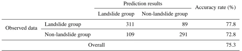
Based on the results of the screening variables, maximum slope, average slope, slope roughness, highest elevation, to-tal slope height, terrain roughness, average aspect subgroup, minimum NDVI, distance from fault, distance from river and lithology type were selected as intrinsic causative factors, as well as the maximum 1 h rainfall and maximum 24 h rain-fall were selected as extrinsic triggering factors. The coef-ficients of variables used in the logistic regression equation are demonstrated in Table 3. The landslide susceptibility map based on the logistic regression model using Typhoon Aere’s rainfall as triggering factors is presented in Fig. 5. The clas-sification error matrix is shown in Table 4, and the SRC and frequency distribution are presented in Fig. 6. The applicabil-ity of the model was confirmed by an accuracy rate of 77.8 % for the landslide group, and an accuracy rate of 72.8 % for the non-landslide group, as well as an AUC value of 0.788, and the separation of the two groups in the frequency distribution plot.
Table 3. Coefficients of variables used in the logistic regression equation.
Variable Coefficient Variable Coefficient Variable Coefficient
Maximum slope 0.036 Maximum 1 h rainfall 0.035 Average aspect
Average slope 0.004 Maximum 24 h rainfall 0.003 Average aspect subgroup (1) 0.646 Slope roughness 0.019 Intercept −8.053 Average aspect subgroup (2) 1.294 Highest elevation 0.001 Lithology Average aspect subgroup (3) 1.340 Total slope height 0.003 Lithology type (1) 1.128 Average aspect subgroup (4) 1.091 Terrain roughness 0.002 Lithology type (2) −0.317 Average aspect subgroup (5) 0.699 Minimum NDVI −2.602 Lithology type (3) −19.364 Average aspect subgroup (6) 0.429 Distance from fault −0.033 Lithology type (4) −19.856 Average aspect subgroup (7) 0.316 Distance from river −0.046
30 1
2
Fig. 4. Maximum 1 h and cumulative 24 h rainfall during Typhoon Aere. 3
4
Fig. 4. Maximum 1 h and cumulative 24 h rainfall during Typhoon Aere.
susceptibility interval. To summarize, the relationship equa-tion was used to convert landslide susceptibility indices to landslide ratios. The results will express the probability of landslides in slope units if identical rainfall conditions oc-curred in future.
31 1
2
Fig. 5. Landslide susceptibility map based on logistic regression model using rainfall of 3
Typhoon Aere as triggering factors. 4
5
Fig. 5. Landslide susceptibility map based on logistic regression model using rainfall of Typhoon Aere as triggering factors.
4.3 Temporal probability of multi-year landslide inventory
The multi-year landslide inventory, as illustrated in Table 1, was used to calculate the temporal probability of landslide occurrence in each slope unit using the Poisson probability model. The inventory covers the temporal interval of nearly 15 yr from 1996 to 2009. After summing the landslide count
32 1
2
Fig. 6. Success rate curve and frequency distribution of landslide and non-landslide groups for 3
the established model. 4
5
AUC=0.788
D=1.386
Fig. 6. Success rate curve and frequency distribution of landslide and non-landslide groups for the established model.
Table 4. Classification error matrix for Typhoon Aere.
Prediction results
Accuracy rate (%) Landslide group Non-landslide group
Observed data Landslide group 311 89 77.8
Non-landslide group 109 291 72.8
Overall 75.3
in each slope unit from 1996 to 2009, the mean recurrence interval (µ)of each slope unit was calculated. Based on the assumption that landslides will occur with the same rate over the next 15 yr as over the past 15 yr, the probability of land-slides during 1, 2, 5, 10, and 15 yr was calculated for each slope unit. Figure 8 demonstrates the probability of landslide occurrence during the next 1 yr period.
Under the assumed conditions, the areas with the highest landslide probability in the Shihmen watershed are those ar-eas that experienced numerous landslides over the past 15 yr. The slope units with the highest landslide probability were clustered in the southwestern part of the watershed.
Furthermore, the landslide probability for the next 1 yr pe-riod was obtained using the Poisson probability model, and could be validated using the subsequent estimated annual probability. The results of this validation are discussed in Sect. 5.
4.4 Cumulative probability of landslide area
A landslide inventory for the research area was used to per-form the landslide size analysis. All new landslides for pre-vious years were divided among three groups according to the slope height of each slope unit. The reason why three groups were analyzed was to testify whether the units with
higher slope height have a higher probability of landslides with large area. The first group consisted of slope units with slope heights of less than 379 m, the second of units with slope heights of 379–514 m, and the third of units with slope heights of more than 514 m. The grouping criteria were deter-mined to ensure similar numbers of slope units in each group. The first group had 4016 landslides with aβvalue of 2.1724; the second, 3985 landslides with aβ value of 2.2546; and the third group had 4007 landslides with aβvalue of 2.1265. The higher theβvalue, the steeper the power law tail will be, thus the lower the ratio of landslides with large areas.
33 1
2
Fig. 7. Landslide spatial probability for the established model. The landslide susceptibility 3
indices of Fig. 5 were converted to landslide spatial probability using the relationship as 4
demonstrated in the upper right corner. 5
6
Fig. 7. Landslide spatial probability for the established model. The landslide susceptibility indices in Fig. 5 were converted to landslide spatial probability using the relationship as demonstrated in the up-per right corner.
1000 m2is approximately 58.3 %, and the probability that the area exceeds 10 000 m2is approximately 6.8 %.
4.5 Validations of spatial and size probabilities
The maximum 1 h rainfall and maximum 24 h rainfall during Typhoon Krosa in 2007 were used as extrinsic triggering fac-tors, in conjunction with the established intrinsic causative factors, to calculate landslide probability maps. The land-slide probability in each slope unit was estimated based on the rainfall conditions that occurred during Typhoon Krosa. To assess the model’s prediction ability, the resulting land-slide spatial probability map was compared with the actual distribution of new landslides analyzed according to the in-ventory before and after Typhoon Krosa.
The landslide susceptibility model had an overall predic-tion accuracy rate of 82.3 % for Typhoon Krosa, which was an excellent result. However, the accuracy rate for the land-slide group was only 62.1 %. This could be attributed to
34 1
2
Fig. 8. The landslide probability during the next 1-year period obtained using the Poisson 3
Probability Model 4
5
Fig. 8. The landslide probability during the next 1 yr period obtained using the Poisson probability model.
35 1
2
Fig. 9. Cumulative probability of landslide area exceeding a certain size threshold based on 3
Pearson Type 5 (3P) Distribution. 4
5
Fig. 9. Cumulative probability of landslide area exceeding a certain size threshold based on Pearson type 5 (3P) distribution.
the fact that rainfall during Typhoon Aere (the basis of this model) was exceptionally heavy. The rainfall was signifi-cantly lighter during Typhoon Krosa, and therefore increased the error rate. Furthermore, the AUC value of the success rate
curve was 0.796, which indicated that all landslides occurred in areas with a relatively high susceptibility. The separation of the landslide group from the non-landslide group in the frequency distribution plot revealed that the model’s parame-ters possessed the ability to distinguish landslides from non-landslides. This result indicated that this model also retained fairly good accuracy under relatively light rainfall conditions, such as the rainfall during Typhoon Krosa.
Furthermore, 611 landslides with new areas greater than 100 m2were caused by Typhoon Krosa. The cumulative per-centages of landslide areas are presented in Fig. 10. A total of 296 landslides had areas greater than 1000 m2, which consti-tuted 48.4 % of all landslides and was less than the predicted 58.3 %. The probability that landslides had areas greater than 1000 m2, caused by a relatively low rainfall event such as Ty-phoon Krosa, was less than 58.3 % predicted using the prob-ability density function. This result indicated that there was a higher than expected proportion of landslides with areas less than 1000 m2. As a consequence, a hazard model based on a Pearson type 5 (3P) probability density function would overestimate the probability of landslides with a certain size under conditions of relatively light rainfall. However, con-cerning hazard assessment, this situation could be considered a conservation result, and the model could still facilitate the identification of problem areas.
5 Results of annual landslide probability
Rainfall data from 24 rain gauge stations were collected and used to perform a frequency analysis. Then, landside prob-abilities corresponding to rainfall events with various recur-rence intervals, including 2, 5, 10, 20, 50, 100 and 200 yr, were derived. Exceedance probabilities for particular rainfall events were used as occurrence probabilities. The landslide probabilities of each slope unit with various recurrence in-tervals and the corresponding exceedance probabilities were drawn as a frequency curve. The area under the curve was integrated as the annual landslide probability for each slope unit.
5.1 Landslide ratio in rainfall events with various recur-rence intervals
The rainfall data of 24 rain gauge stations in the vicinity of the study area collected from 1987 to 2009 was used to analyze rainfall amounts of rainfall events with various du-rations and various recurrence intervals. Subsequently, the maximum 1 h rainfall and maximum 24 h rainfall with var-ious recurrence intervals, including 2, 5, 10, 20, 50, 100 and 200 yr, were obtained. Geostatistical methods were sequen-tially used to estimate the maximum 1 h rainfall and max-imum 24 h rainfall throughout the entire area with differ-ent recurrence intervals. These results were used in conjunc-tion with the already-determined intrinsic causative factors
36 1
2
Fig. 10. Cumulative percentage of landslide area for the landslides caused by Typhoon Krosa 3
in 2007. 4 5
Fig. 10. Cumulative percentage of landslide area for the landslides caused by Typhoon Krosa in 2007.
to calculate landslide probability maps for the entire area. These maps demonstrated the landslide probabilities with 2, 5, 10, 20, 50, 100 and 200 yr recurrence intervals, respec-tively. However, because the maximum values at each rain gauge station were used to estimate the spatial distribution of maximum 1 and 24 h rainfall, the resulting landslide suscep-tibilities simultaneously reflected the maximum rainfall val-ues for all stations. These could be regarded as “worst case” prediction results.
5.2 Annual landslide ratio
The landslide probabilities derived from rainfall events with various recurrence intervals represented the landslide proba-bility of each slope unit following such an event. However, it was difficult to derive the occurrence probabilities of the events. In these circumstances, the analysis of the occurrence probability of triggering factors could be used as an alterna-tive method. Therefore, the exceedance probability of rain-fall events with various recurrence intervals was used as the occurrence probability of the events. Additionally, the land-slide probabilities of each slope unit with 2, 5, 10, 20, 50, 100 and 200 yr recurrence intervals, as well as the corresponding exceedance probabilities were drawn as a frequency curve. The area under the curve was integrated as the annual land-slide probability for each slope unit, and the annual landland-slide probability map in the study area was drawn (Fig. 11). The highest landslide probability (the annual landslide probabil-ity of approximately 40 %) was distributed over the Taigang River watershed, the south of this watershed, compared to a probability of less than 10 % in most areas.
5.3 Validation of temporal probability
37 1
2
Fig. 11. Annual landslide probability obtained conjugating the results of rainfall events with 3
various recurrence intervals. 4
5
Fig. 11. Annual landslide probability obtained conjugating the re-sults of rainfall events with various recurrence intervals.
landslides will occur at the same rate over the next 15 yr as over the past 15 yr, the probability of landslide occurrence for each slope unit during the next 1 yr period were obtained (Fig. 8). In addition, annual landslide probabilities were ob-tained using the landslide probabilities of each slope unit with various recurrence intervals, as well as the correspond-ing exceedance probabilities as demonstrated in Fig. 11. The difference between these two was calculated using the annual landslide probability minus the Poisson landslide probability for each slope unit (Fig. 12).
Figure 12 demonstrates that the absolute values of the probability differentials were nearly less than 0.15, which indicate a ratio exceeding 91.9 %. This result indicated that the estimated annual landslide probabilities were extremely close to the estimated 1 yr landslide probabilities. Addition-ally, the feasibility of the use of exceedance probability as the basis to determine the temporal probability of event-based landslides was verified.
38 1
2
Fig. 12. The difference between the annual landslide probability (Fig. 11) and Poisson 3
Landslide Probability (Fig. 8). 4
5
Fig. 12. The difference between the annual landslide probability (Fig. 11) and Poisson landslide probability (Fig. 8).
5.4 Annual probability of landslides exceeding a certain area
The annual probability of landslides exceeding a certain area in any slope unit could be derived with further analysis of the annual landslide probability and landslide area probabil-ity in the Shihmen watershed. For instance, Fig. 13 demon-strates the annual probability of landslides with areas ex-ceeding 3000 m2in each slope unit. The resulting landslide probability model can be used as a basis for future land-slide risk analyses. Furthermore, the annual risk can be es-timated based on the annual landslide probability instead of a scenario-based probability. Thus, the annual benefit of a risk reduction program can be evaluated as the reduced an-nual risk, and the benefit–cost analysis of the program can be successively conducted. In addition, future research could analyze the sediment delivery ratio of each slope unit to esti-mate the volume of sediment transported downstream during landslide events.
39 1
2
Fig. 13. Annual landslide probability for landslide with area exceeding 3,000m2 in each slope 3
unit. 4
Fig. 13. Annual landslide probability for landslides with area ex-ceeding 3000 m2in each slope unit.
6 Conclusions
Climate change enlarges bare land areas and therefore also the number of landslides in Taiwan. In view of a grow-ing emphasis on risk management, the quantitative assess-ment of landslide risk is becoming increasingly important. Scenario-based risks can be estimated using scenario-based landslide probability models, but few annual landslide proba-bility models existed for Taiwan. Therefore, a landslide haz-ard model that can be used to estimate the annual landslide probability, and perform an annual landslide risk analysis was established in this study.
The landslide spatial, temporal and size probabilities were analyzed based on the landslide inventory caused by ty-phoons from 1996 to 2009, 13 variables of landslide sus-ceptibility factors, and rainfall data of those events. These probabilities were integrated to estimate the annual probabil-ity of each slope unit with a landslide area exceeding a cer-tain threshold in the Shihmen watershed. The results demon-strated that the south of this watershed is especially prone to landslides and should therefore be the primary target of future soil conservation efforts.
An overall accuracy rate of 75.3 % and an AUC value of 0.788 confirmed the applicability of the landslide susceptibil-ity model. The AUC value was far greater than the AUC val-ues of the various landslide thematic variables, which high-lighted that the ability of this landslide susceptibility model to predict landslides was more efficient than a model based on only one variable. The validation result of Typhoon Krosa demonstrated that this landslide susceptibility model could be used to predict the spatial probability of landslides caused by rainfall events with various recurrence intervals, including 2, 5, 10, 20, 50, 100 and 200 yr. The landslide area probabil-ity was analyzed using the Pearson type 5 probabilprobabil-ity densprobabil-ity function based on all new landslides from 1996 to 2009. The results suggested that when a landslide occurs in any slope unit within the Shihmen watershed, the probability that the landslide area will exceed 10 000 m2is approximately 6.8 %. The difference between the annual landslide probability and the Poisson landslide probability for each slope unit was compared to verify the feasibility of the use of ex-ceedance probability to determine the temporal probability of event-based landslides. The newly established annual land-slide probability model could be used for future landland-slide risk analysis. This method avoids inconsistencies that exist between the assumptions of the Poisson probability model and the real situation. Especially when the landslide inven-tory relies on a limited time period, the assumption that land-slides will occur with the same rate over the next few years as over the past can result in a future landslide probability of 0 in a slope unit if it did not have landslides in the past. The advantages of this annual landslide probability model are the ability to estimate the annual landslide risk instead of a scenario-based risk, and the need of landslide data from few events instead of a long-term inventory. Furthermore, the annual benefit of a risk reduction program can be evaluated as the reduced annual risk, and the benefit–cost analysis of the program can be successfully conducted in Taiwan. The resulting model is feasible to estimate the annual probability of each slope unit with a landslide area exceeding a certain threshold. We suggest it may be further developed so that the location where a landslide will most likely occur in each slope unit could be included.
Acknowledgements. The authors would like to thank the National
Science Council, Taiwan, for financially supporting this research (NSC 101-2811-M-005-033). The Soil and Water Conservation Bureau and involved counties are commended for their full cooperation.
Edited by: P. Tarolli
References
Baeza, C. and Corominas, J.: Assessment of shallow landslide sus-ceptibility by means of multivariate statistical techniques, Earth Surf. Proc. Landf., 26, 1251–1263, 2001.
Bak, P., Tang, C., and Wiesenfeld, K.: Self-organized criticality, Phys. Rev., A38, 364–374, 1988.
Bründl, M., Romang, H. E., Bischof, N., and Rheinberger, C. M.: The risk concept and its application in natural hazard risk man-agement in Switzerland, Nat. Hazards Earth Syst. Sci., 9, 801– 813, doi:10.5194/nhess-9-801-2009, 2009.
Carrara, A.: A multivariate model for landslide hazard evaluation, Math. Geol., 15, 403–426, 1983.
Carrara, A., Crosta, G., and Frattini, P.: Comparing models of debris-flow susceptibility in the alpine environment, Geomor-phology, 94, 353–378, 2008.
Cavalli, M., Tarolli, P., Marchi, L., and Dalla Fontana, G.: The ef-fectiveness of airborne LiDAR data in the recognition of channel bed morphology, Catena, 73, 249–260, 2008.
Central Geological Survey: Landslide susceptibility zonation in slopeland of urban area, Sinotech Engineering Consultants Inc., 2009 (in Chinese).
Chen, S. C. and Huang, B. T.: Non-structural mitigation programs for sediment-related disasters after the Chichi Earthquake in Tai-wan, J. Mountain Sci., 7, 291–300, 2010.
Chen, S. C., Wu, C. Y., and Huang, B. T.: The efficiency of a risk reduction program for debris-flow disasters – a case study of the Songhe community in Taiwan, Nat. Hazards Earth Syst. Sci., 10, 1591–1603, doi:10.5194/nhess-10-1591-2010, 2010.
Chen, Y. R., Ni, P. N., and Tsai, K. J.: Construction of a sediment disaster risk assessment model, Environ. Earth Sci., 70, 115–129, 2013.
Chung, C. F. and Fabbri, A.: The representation of geoscience in-formation for data integration, Nonrenew Resour., 2, 122–138, 1993.
Chung, C. F. and Fabbri, A. G.: Probabilistic prediction models for landslide hazard mapping, Photogram. Eng. Remote Sens., 65, 1389–1399, 1999.
Crovelli, R. A.: Probability models for estimation of number and costs of landslides, United States Geological Survey Open File Report 00-249, 2000.
Dahal, R. K., Hasegawa, S., Nonomura, A., Yamanaka, M., Dhakal, S., and Paudyal, P.: Predictive modelling of rainfall-induced landslide hazard in the Lesser Himalaya of Nepal based on weights-of-evidence, Geomorphology, 102, 496–510, 2008. David, R. M.: Arc Hydro: GIS for Water Resources, ESRI Press,
Redlands, CA., 2002.
Fujii, Y.: Frequency distribution of landslides caused by heavy rain-fall, J. Seismol. Soc. Jpn., 22, 244–247, 1969.
Ghosh, S., van Westen, C. J., Carranza, E. J. M., and Jetten, V. G.: Integrating spatial, temporal, and magnitude probabilities for medium-scale landslide risk analysis in Darjeeling Himalayas, India, Landslides, 9, 371–384, 2012a.
Ghosh, S., van Westen, C. J., Carranza, E. J. M., Jetten, V. G., Car-dinali, M., Rossi, M., and Guzzetti, F.: Generating event-based landslide maps in a data-scarce Himalayan environment for es-timating temporal and magnitude probabilities, Eng. Geol., 128, 49–62, 2012b.
Guzzetti, F., Carrara, A., Cardinali, M., and Reichenbach, P.: Land-slide hazard evaluation: an aid to a sustainable development, Ge-omorphology, 31, 181–216, 1999.
Guzzetti, F., Malamud, B. D., Turcotte, D. L., and Reichenbach, P.: Power-law correlations of landslide areas in central Italy, Earth Planet. Sci. Lett., 195, 169–183, 2002.
Guzzetti, F., Reichenbach, P., Cardinali, M., Galli, M., and Ardiz-zone, F.: Probabilistic landslide hazard assessment at the basin scale, Geomorphology, 72, 272–299, 2005.
Guzzetti, F., Galli, M., Reichenbach, P., Ardizzone, F., and Cardi-nali, M.: Landslide hazard assessment in the Collazzone area, Umbria, Central Italy, Nat. Hazards Earth Syst. Sci., 6, 115–131, doi:10.5194/nhess-6-115-2006, 2006.
Hovius, N., Stark, C. P., Chu, H. T., and Lin, J. C.: Supply and re-moval of sediment in a landslide-dominated mountain belt: Cen-tral Range, Taiwan, J. Geol., 108, 73–89, 2000.
Jaiswal, P., van Westen, C. J., and Jetten, V.: Quantitative assess-ment of landslide hazard along transportation lines using histori-cal records, Landslides, 8, 279–291, 2011.
Lee, C.-T., Huang, C.-C., Lee, J.-F., Pan, K. -L., Lin, M.-L., and Dong, J.-J.: Statistical approach to storm event-induced land-slides susceptibility, Nat. Hazards Earth Syst. Sci., 8, 941–960, doi:10.5194/nhess-8-941-2008, 2008.
Lin, Y. H.: Application of neural network to landslide susceptibil-ity analysis, Master thesis, National Central Universsusceptibil-ity, Taiwan, 2003 (in Chinese).
Malamud, B. D., Turcotte, D. L., Guzzetti, F., and Reichenbach, P.: Landslide inventories and their statistical properties, Earth Surf. Proc. Landf., 29, 687–711, 2004.
Nefeslioglu, H. A. and Gokceoglu, C.: Probabilistic risk assessment in medium scale for rainfall-induced earthflows: Catakli Catch-ment Area, Mathe. Problems Eng., 2011, 1–21, 2011.
Onoz, B. and Bayazit, M.: Effect of the occurrence process of the peaks over threshold on the flood estimates, J. Hydrol., 244, 86– 96, 2001.
Rossi, M., Guzzetti, F., Reichenbach, P., Mondini, A. C., and Pe-ruccacci, S.: Optimal landslide susceptibility zonation based on multiple forecasts, Geomorphology, 114, 129–142, 2010. Stark, C. P. and Hovius, N.: The characterization of landslide size
distributions, Geophys. Res. Lett., 28, 1091–1094, 2001. Van Den Eeckhaut, M., Reichenbach, P., Guzzetti, F., Rossi, M.,
and Poesen, J.: Combined landslide inventory and susceptibility assessment based on different mapping units: an example from the Flemish Ardennes, Belgium, Nat. Hazards Earth Syst. Sci., 9, 507–521, doi:10.5194/nhess-9-507-2009, 2009.
Varnes, D. J. and IAEG Commission on Landslides and other Mass-Movements: Landslide hazard zonation: a review of principles and practice, NESCO Press, Paris, 1984.
Weng, K. L.: Types and distribution of landslides in the Yufong River watershed, Master thesis, National Chung-Hsing Univer-sity, Taiwan, 2009 (in Chinese).
Wilson, J. P. and Gallant, J. C.: Terrain analysis – principles and applications. John Wiley & Sons, New York, 2000.
Wu, C. H. and Chen, S. C.: Determining landslide susceptibility in Central Taiwan from rainfall and six site factors using the analyt-ical hierarchy process method, Geomorphology, 112, 190–204, 2009.
Xie, M., Esaki, T., and Zhou, G.: Gis-based probabilistic map-ping of landslide hazard using a three-dimensional deterministic model, Nat. Hazards, 33, 265–282, 2004.