University of Pennsylvania
ScholarlyCommons
Publicly Accessible Penn Dissertations
1-1-2016
Studying the Large Scale Structure and interstellar
Medium of Galaxies During the Epochs of Peak
Cosmic Star formation and Reionization With
Infrared Fine Structure Lines
Bade D. Uzgil
University of Pennsylvania, badeuzgil@gmail.com
Follow this and additional works at:http://repository.upenn.edu/edissertations
Part of theAstrophysics and Astronomy Commons
This paper is posted at ScholarlyCommons.http://repository.upenn.edu/edissertations/2070
For more information, please contactlibraryrepository@pobox.upenn.edu.
Recommended Citation
Uzgil, Bade D., "Studying the Large Scale Structure and interstellar Medium of Galaxies During the Epochs of Peak Cosmic Star formation and Reionization With Infrared Fine Structure Lines" (2016).Publicly Accessible Penn Dissertations. 2070.
Studying the Large Scale Structure and interstellar Medium of Galaxies
During the Epochs of Peak Cosmic Star formation and Reionization With
Infrared Fine Structure Lines
Abstract
Infrared (IR) fine-structure (FS) lines from trace metals in the interstellar medium (ISM) of galaxies are valuable diagnostics of the physical conditions in a broad range of astrophysical environments, such gas irradiated by stellar far-ultraviolet (FUV) photons or X-rays from accreting supermassive black holes, called active galactic nuclei (AGN). The transparency of these lines to dust and their high escape fractions into the intergalactic medium (IGM) render them as useful probes to study the epochs of peak cosmic star formation (SF) and Reionization.
Chapter 1 of this thesis is a study of the ISM of the Cloverleaf quasar. Observations of IR FS lines from singly ionized carbon and neutral oxygen have allowed us to assess the physical conditions—parametrized by their gas density and the impingent FUV flux—prevalent in atomic gas heated by stellar FUV photons. We find that UV heating from local SF is not sufficient to explain the measured FS and molecular luminosities, and suggest that X-ray heating from the AGN is required to simultaneously explain both sets of data. The general picture of the Cloverleaf ISM that emerges from our composite model is one where the [CII] and [OI]63 line emission is produced primarily within PDRs and HII regions of a 1.3-kpc wide starburst, which is embedded in a denser XDR component that is the dominant source of heating for the CO gas. The fact that the star-forming PDR and HII region gas is co-spatial with the XDR—and within ∼ 650 pc of the accreting black
hole—provides strong evidence that SF is ongoing while immersed in a strong X-ray radiation field provided by the nearby AGN. This finding has implications for the co-evolution of supermassive black holes and their host galaxies. The work in this chapter will be submitted for first-author publication imminently.
In Chapter 2, we explore the possibility of studying the redshifted far-IR fine-structure line emission using the three-dimensional (3-D) power spectra obtained with an imaging spectrometer. The intensity mapping approach measures the spatio-spectral fluctuations due to line emission from all galaxies, including those below the individual detection threshold. The technique provides 3-D measurements of galaxy clustering and moments of the galaxy luminosity function. Furthermore, the linear portion of the power spectrum can be used to measure the total line emission intensity including all sources through cosmic time with redshift information naturally encoded. Total line emission, when compared to the total star formation activity and/or other line intensities reveals evolution of the interstellar conditions of galaxies in aggregate. As a case study, we consider measurement of [CII] autocorrelation in the 0.5 < z < 1.5 epoch, where interloper lines are
minimized, using far-IR/submm balloon-borne and future space-borne instruments with moderate and high sensitivity, respectively. In this context, we compare the intensity mapping approach to blind galaxy surveys based on individual detections. We find that intensity mapping is nearly always the best way to obtain the total line emission because blind, wide-field galaxy surveys lack sufficient depth and deep pencil beams do not observe enough galaxies in the requisite luminosity and redshift bins. Also, intensity mapping is often the most efficient way to measure the power spectrum shape, depending on the details of the luminosity function and the telescope aperture. The work in this chapter has been published in Uzgil et al. (2014).
spectrum during the same epoch, as the former is a direct probe of the sources of Reionization, and the latter is a probe of the effect of those sources on the surrounding IGM. Since current and planned observations are limited by cosmic variance at the bright end of the galaxy luminosity function, and will not be able to detect the faintest galaxies responsible for a significant fraction of the ionizing photon supply during EoR, intensity mapping is an appealing approach to study the nature and evolution of galaxies during this stage in the history of the Universe. Again, the utility of FS lines as ISM diagnostics, combined with the ability of intensity mapping to measure redshift-evolution in mean intensity of individual lines or the evolution of line ratios (constructed from multiple cross-power spectra), presents a unique and tantalizing opportunity to directly observe changes in properties of interstellar medium (such as hardness of the ionizing spectrum in galaxies and metallicity) that are important to galaxy evolution studies.
Degree Type
Dissertation
Degree Name
Doctor of Philosophy (PhD)
Graduate Group
Physics & Astronomy
First Advisor
James E. Aguirre
Second Advisor
Charles M. Bradford
Subject Categories
STUDYING THE LARGE SCALE STRUCTURE AND
INTERSTELLAR MEDIUM OF GALAXIES DURING THE
EPOCHS OF PEAK COSMIC STAR FORMATION AND
REIONIZATION WITH INFRARED FINE STRUCTURE LINES
Bade D. Uzgil
A DISSERTATION
in
Physics & Astronomy
Presented to the Faculties of the University of Pennsylvania in Partial
Fulfillment of the Requirements for the Degree of Doctor of Philosophy
2016
Supervisor of Dissertation
Co-Supervisor of Dissertation
James E. Aguirre, Professor
Charles M. Bradford, Doctor
Graduate Group Chairperson
Marija Drndic, Professor
Dissertation Committee:
ABSTRACT
STUDYING THE LARGE SCALE STRUCTURE AND INTERSTELLAR
MEDIUM OF GALAXIES DURING THE EPOCHS OF PEAK COSMIC STAR
FORMATION AND REIONIZATION WITH INFRARED FINE STRUCTURE
LINES
Bade D. Uzgil
James E. Aguirre
Charles M. Bradford
Infrared (IR) fine-structure (FS) lines from trace metals in the interstellar medium (ISM) of galaxies are valuable diagnostics of the physical conditions in a broad range of astrophysical environments, such gas irradiated by stellar far-ultraviolet (FUV) photons or X-rays from accreting supermassive black holes, called active galactic nuclei (AGN). The transparency of these lines to dust and their high escape frac-tions into the intergalactic medium (IGM) render them as useful probes to study the epochs of peak cosmic star formation (SF) and Reionization.
Chapter 1 of this thesis is a study of the ISM of the Cloverleaf quasar. Obser-vations of IR FS lines from singly ionized carbon and neutral oxygen have allowed us to assess the physical conditions—parametrized by their gas density and the impingent FUV flux—prevalent in atomic gas heated by stellar FUV photons. We find that UV heating from local SF is not sufficient to explain the measured FS and molecular luminosities, and suggest that X-ray heating from the AGN is required to simultaneously explain both sets of data. The general picture of the Cloverleaf ISM that emerges from our composite model is one where the [CII] and [OI]63 line emission is produced primarily within PDRs and HII regions of a 1.3-kpc wide starburst, which is embedded in a denser XDR component that is the dominant source of heating for the CO gas. The fact that the star-forming PDR and HII region gas is co-spatial with the XDR—and within ∼650 pc of the accreting black hole—provides strong evidence that SF is ongoing while immersed in a strong X-ray radiation field provided by the nearby AGN. This finding has implications for the co-evolution of supermassive black holes and their host galaxies. The work in this chapter will be submitted for first-author publication imminently.
fine-structure line emission using the three-dimensional (3-D) power spectra obtained with an imaging spectrometer. The intensity mapping approach measures the spatio-spectral fluctuations due to line emission from all galaxies, including those below the individual detection threshold. The technique provides 3-D measurements of galaxy clustering and moments of the galaxy luminosity function. Furthermore, the linear portion of the power spectrum can be used to measure the total line emis-sion intensity including all sources through cosmic time with redshift information naturally encoded. Total line emission, when compared to the total star formation activity and/or other line intensities reveals evolution of the interstellar conditions of galaxies in aggregate. As a case study, we consider measurement of [CII] au-tocorrelation in the 0.5 < z < 1.5 epoch, where interloper lines are minimized, using far-IR/submm balloon-borne and future space-borne instruments with mod-erate and high sensitivity, respectively. In this context, we compare the intensity mapping approach to blind galaxy surveys based on individual detections. We find that intensity mapping is nearly always the best way to obtain the total line emis-sion because blind, wide-field galaxy surveys lack sufficient depth and deep pencil beams do not observe enough galaxies in the requisite luminosity and redshift bins. Also, intensity mapping is often the most efficient way to measure the power spec-trum shape, depending on the details of the luminosity function and the telescope aperture. The work in this chapter has been published in Uzgil et al. (2014).
Contents
1 Constraining ISM properties of the Cloverleaf Quasar with
Her-schel spectroscopy 1
1.1 Introduction . . . 1
1.2 Observations . . . 3
1.2.1 Extinction corrections . . . 7
1.3 Analysis . . . 7
1.3.1 [CII]158µm from non-star-forming gas . . . 8
1.3.2 Star-forming ISM: PDRs and stellar HII regions . . . 10
1.3.3 X-ray dominated region . . . 16
1.3.4 Alternative heating sources . . . 24
1.4 Discussion . . . 27
1.4.1 Molecular clump sizes and spatial distribution . . . 27
1.4.2 Comparison with high-redshift and local systems . . . 28
1.5 Conclusions . . . 29
2 Measuring galaxy clustering and the evolution of [CII] mean in-tensity with Far-IR line inin-tensity mapping during 0.5 < z <1.5 33 2.1 Introduction . . . 33
2.2 Predictions for Far-IR Line Power Spectra . . . 35
2.2.1 Relationship Between Galaxy Populations and Fluctuation Power . . . 35
2.2.2 Calculating IR line volume emissivity . . . 36
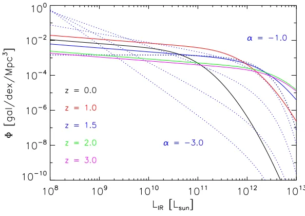
2.2.3 [CII] Luminosity Functions and Expected Power Spectra . . 41
2.3 The [CII] Power Spectrum . . . 44
2.3.1 Observational Sensitivity to the Power Spectrum . . . 44
2.3.2 Measuring Line Luminosity Density Over Cosmic Time . . . 49
2.4 Observational Strategy: Comparing Intensity Mapping with Tradi-tional Galaxy Surveys . . . 52
2.4.1 Probes of the mean line intensity . . . 52
2.4.2 Probes of the power spectrum . . . 56
3 FS Line Intensity Mapping During the Epoch of Reionization 61
4 Conclusion 68
Appendices 69
A Appendix to the Preface 70
B Appendix to Chapter1 85
Preface
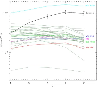
The study of cosmology versus the study of astrophysics is the study of the whole versus its parts, of the Universe versus its occupants, of, for example, the accel-eration of space-time versus the ignition of supernovae. Certain questions are better addressed, undeniably, in one field and not the other—“Do we live in a multiverse?”—but some are fully understood only where the two fields intersect. One such question, of particular relevance to this thesis, concerns the origin and evolution of galaxies, such as our own Milky Way or our neighbors, Messier 82 (M 82) and Markarian 231 (Mrk 231).1
In order to discuss the evolution of galaxies from a purely cosmological perspec-tive, it is first necessary to trade in the notion of a galaxy as a vast collection of stars, gas, and dust for a more austere definition, namely, a perturbation ∆ρρ in den-sity ρ. Indeed, it is a remarkable fact that all large-scale structure observed in the present Universe—from individual galaxies and superclusters (containing, say, some 105 galaxies) to the filaments and voids of the “cosmic web”—trace their origins to tiny fluctuations in density when the Universe was only a fraction of a second old; and, this fact is one of the predictions of the current most successful cosmological model.
The current model, however, cannot predict precisely the level of density per-turbations in the early Universe which gave rise to the present assembly of mass in various observed structures. Instead, observations pin the order of density pertur-bations to ∆ρρ ∼10−5 at a time when the Universe was roughly 3.7×10⁵ years old, corresponding to a time when the equilibrium between photons, protons, electrons, and hydrogen atoms was broken such that neutral hydrogen could outnumber elec-trons and protons. From then on, photons could decouple from matter,2 expand with the Universe, cool from∼3000 K to 2.7 K, and eventually reach telescopes to-day as the Cosmic Microwave Background (CMB). The formation of the CMB, also referred to simply as “decoupling” or “recombination,” marks a critical stage in the Universe’s evolution, as neutral hydrogen is produced in abundance and will begin to collapse rapidly when the energy density of matter dominates over radiation in the Universe. (In fact, the collapse of all kinds of matter, including non-baryonic
1Here, “neighbor” is meant strictly in the astronomical sense. M 82 is located 2.9 Mpc =
matter, commences after decoupling because the speed of sound ceases to be rela-tivistic.) If we suppose that matter consists entirely of baryons, then simply evolving the density perturbations—imprinted in the CMB as fluctuations in temperature
∆T
T ∼ 10
−5—to grow in time as expected for a matter-dominated Universe, i.e.,
allowing them to grow linearly with the cosmological expansion, under-predicts the observed range of density fluctuations today, which can be as high as ∆ρρ ∼10−102 for galaxy clusters (returning to the astrophysicist’s parlance). The inclusion of a significant non-relativistic, or cold, dark matter (DM) component into the cur-rent cosmological model, which we can now refer to somewhat meaningfully as the Λ-CDM model,3 means, for example, that matter-domination occurs at an earlier time, giving perturbations more time to grow; since DM, by nature, does not in-teract with radiation, the perturbations in the DM density field also tend to grow more efficiently.
Once the amplitudes of density perturbations become large enough, their growth is no longer linear, and can be computed with N-body simulations (e.g., Springel et al. (2005)) that account for gravitational interactions between large numbers of particles. Alternatively, the nonlinear development of perturbations can be de-scribed with theories of collapse for spheroids (Press & Schechter 1974; White & Rees 1978) or, more accurately, ellipsoids (Sheth et al. 2001), in which matter col-lapses to smaller radii and forms gravitationally bound objects in virial equilibrium, with the virial mass, M, at the time of collapse becoming progressively larger at later times—an example of the hierarchical growth that governs the formation of structures in the Universe. The DM collapses first because the amplitude of ∆ρρ in the DM density field was already larger than 10−5 at the formation of the CMB due to the premature growth of perturbations during the radiation-dominated era, forming bound objects called halos. These halos served as hosts for the formation of stars and later galaxies as baryons proceeded to accumulate in the attractive gravitational potential of the DM. Through gravitational interactions and mergers, the halos and baryons accumulate mass, exemplifying further the principle of hier-archical structure growth that ultimately results in the large-scale structure of the cosmos observed today.
Therefore, in the broad sense that galaxies initially formed from the collapse of baryons in DM halos, their evolution is inextricably linked to that of their hosts. While the abundance, spatial clustering, mass distribution, and other key properties of DM halos can be described with analytic theories (cf. Cooray & Sheth (2002) for a summary) introduced above, simply assuming that galaxies and DM halos follow the same evolutionary path—one that is theoretically well understood—leads to a number of predictions that do not agree with observations, such as the history of star formation in the Universe.
3Λ denotes the small, but non-zero cosmological constant which drives the observed acceleration
Star formation in galaxies and dark matter halos The star formation rate (SFR, units of M yr−1) is a useful indicator of a galaxy’s evolutionary phase.
According to observations (e.g., Daddi et al. (2007), Elbaz et al. (2011)) in the nearby and distant Universe, there is a correlation between a galaxy’s stellar mass and its SFR (per unit stellar mass4). Galaxies may spend the most time in a phase where they form stars in line with this correlation—called the galaxy “main sequence”—compared to relatively short-lived phases during which star formation is enhanced (i.e., undergoing a “starburst” phase, as in M 82) and suppressed. Measurements of the space density of star formation, ρSFR(M yr−1 Mpc−3), in the
Universe across cosmic timescales (i.e., on the order ∼109−10 yr = 1−10 Gyr) are a means of piecing together a global view of galaxy evolution (Madau & Dickinson 2014).
Suppose, then, that the evolution of DM halos is sufficient to describe the cosmic history of star formation. If galaxies merely follow the DM halo evolution, without any additional astrophysical processes involved, then the relation between SFR and DM halo mass should maintain a simple linear dependence. Then it is possible to use theoretical predictions for the number, or fraction, fcoll, of halos greater than
a given mass, Mmin, that have collapsed at a given time, or redshift z,5 in the
Universe’s history in order to predict ρSFR at that time:
ρSFR(z)∝fcoll(M > Mmin;z) ¯ρ(z)/tH(z), (0.0.1)
where ¯ρ(z) is the redshift-dependent average background density of DM in the Uni-verse, and tH(z) is the age of the Universe at z, i.e., the Hubble time at z. To calculate fcoll(M > Mmin;z), we have used the Sheth-Tormen halo mass function
(Sheth et al. 2001), dMdNdV, which describes the average number N of DM halos between a mass M and M+ dM per infinitesimal unit of (comoving6) volume dV. The righthand panel of Figure 1 shows the resulting evolution of ρSFRwith redshift, as well as empirically-based models from Robertson et al. (2015) and Hopkins & Beacom (2006a). The integral of ρSFR over the time spanned by this toy model has been normalized to match the integral of ρSFR reported in Robertson et al. (2015), since here we are mainly interested in whether the shape of the cosmic history of
4The SFR that is normalized by a galaxy’s stellar mass is often referred to as the specific SFR
(sSFR).
5Note that units of time are expressed in terms of redshift, z, which is defined in relation to
the scale factor, a(t), of the Universe: z = a(at(=0)t) −1. The scale factor describes the extent to which a physical length dhas been stretched from its present lengthd0 due to the expansion of
the Universe at a given timet, such thatd=a(t)d0, witha(t= 0) = 1 (and hencez= 0) locally.
Because the wavelength,λem, of radiation emitted at a timetis similarly stretched by cosmological expansion, spectroscopy offers observers a useful means of identifying a source’s redshift from its spectral line emission.
6A “comoving” distance in cosmology is used to refer to distances between objects that have
Figure 1: Cosmic star formation rate density,ρSFR, as a function of redshift,z. (left): Blue and
red data points indicate UV and IR luminosity densities, ρUVandρIR, respectively, converted to ρSFR with prescriptions from Madau & Dickinson (2014) and Kennicutt (1998a). The respective
luminosity densities have been calculated by integrating observed luminosity functions down to 0.001 times the characteristic galaxy luminosity at a given redshift,L∗, as defined in the Schechter
or double power-law formalism. The white line represents the maximum likelihood model forρSFR,
with 1σconfidence region highlighted in red, when fitting a model to the data with the constraint that the model reproduces the Planck satellite’s measurement of the Thomson optical depth,τe,
assuming that the cosmic ionization rate is proportional to the cosmic star formation rate density.
Dashed blue curve shows the maximum likelihood model of ρSFR when the Planck constraint
is ignored. The orange swath is the result when the model is forced to match τe measured by
WMAP. Figure from Robertson et al. (2015). (right): Models forρSFR(z) according to Robertson
et al. (2015) (red curve; same as white curve in left panel of this Figure) and Hopkins & Beacom (2006a) (green curve). Assuming that star formation rate is linearly related to DM halo mass,
M—with constant of proportionality betweenρSFR and M determined by forcing the integrated
SFR density (in the interval 0≤z≤10) to equal that of the Robertson et al. (2015) model—and applying the halo mass function from Sheth et al. (2001) to determine the population of DM halos with mass greater than Mmin as a function of redshift, yields the cosmic star formation rate histories shown as the dashed curves. Different curves correspond to different assumptions regarding the the minimum mass,Mmin=MSF,min, at which a DM halo can begin forming stars,
ρSFR matches the observed trend with redshift; the prescribed dependence on ρSFR with M is linear, anyway, and so the amplitude can be forced to agree with ob-servations by changing the constant of proportionality between them. This simple model of galaxy evolution is only sensitive to the mass at which a halo can begin forming stars, denoted MSF,min. For example, halo masses between ∼108–109 M
are physically-motivated choices for Mmin = MSF,min, as these masses correspond
to virial temperatures in the halo that ionize hydrogen and allow the gas to cool radiatively,7 which, in turn, allows the gas to contract further and potentially form stars. In any case, the peak in cosmic star formation activity occurs when the frac-tion of mass contained in virialized DM halos of mass MSF,min is at a maximum,
which happens at progressively later times (i.e., lower redshifts) for larger values of MSF,min. Importantly, there is no single choice of MSF,min that matches the
ob-served history of ρSFR. This disagreement suggests that the relation between SF
and halo mass is highly non-linear, and that the star formation efficiency changes
with halo mass. The sources of this non-linearity are the complex astrophysical
processes between baryons which we neglected in our toy model, but which govern the evolution of galaxies in addition to the gravitational influence of DM halo envi-ronment. Triggers of starburst activity, for example, which raise galaxies above the star-forming “main sequence,” could be the result of galaxy-galaxy mergers or infall of cold gas into galaxies from DM halos. Feedback between accreting supermassive black holes at the centers of galaxies, called active galactic nuclei (AGN), and star-forming gas also appears to be play an important role in galaxy evolution—possibly a mechanism for regulating SF—and will be explored in Chapter 1 of this thesis.
Studies that target the Universe when it was approximately between 2 and 6 billion years old (or, betweenz ≈ 3 and 1, respectively) probe a critical time frame in the evolution of galaxies, corresponding to the peak of cosmic SF as indicated in Figure 1, i.e, when galaxies appear to have been the most active in forming stars; ρSFR in this redshift range is 10 times higher than in the local (z ∼ 0) Universe. SFR estimates in the lefthand panel of Figure 1 have been calculated from luminosity densities of ultraviolet (ρUV; blue data points) and infrared (ρIR; red data points) light rom galaxies, using prescriptions that take into account the correlation between a galaxy’s UV and IR luminosities and its SFR (Madau & Dickinson 2014; Kennicutt 1998a). In the presence of interstellar dust, UV radiation from the gas within a galaxy is reduced from its intrinsic luminosity because it is readily absorbed by the dust grains, and re-emitted at IR wavelengths. Thus, while the observed UV luminosity of a galaxy indicates the energy output of its stellar populations—these are the primary sources of Lyman continuum photons8 in purely star-forming systems—ρUV can lead to an underestimate ofρSFRfor dusty star-forming galaxies (DSFGs) unless the correct extinction factors are applied. In Figure 2, the increasing fraction with redshift of SF in dust-rich environments
7via hydrogen recombinations andbremsstrahlung
Figure 2: Cosmic star formation rate density (ρSFR, or SFRD; green curve) as a function of
redshift, deconstructed into contributions from SFRD as measured fromρIR(red curve) andρUV
(blue curve). UV luminosity densities in this Figure have not been corrected for extinction by dust. Figure from Burgarella et al. (2013a).
is illustrated by comparing ρSFR inferred from the measured (i.e., uncorrected for dust extinction) UV and IR emission from galaxies. By a redshift of z ∼ 0.5, the so-called “hidden,” or dust-obscured, fraction of ρSFR is already 80%, and remains between 75−90% throughout the epoch of peak SF activity (Burgarella et al. 2013a). The relative importance of obscured SF in this cosmic epoch motivates the need to understand the nature of extinction in these sources, and to have independent measures ofρIR for a more accurate bolometric estimate of SF. Furthermore, it also highlights the utility, in general, of probes of the SF process in galaxies during this cosmic epoch that are not significantly extincted by dust.
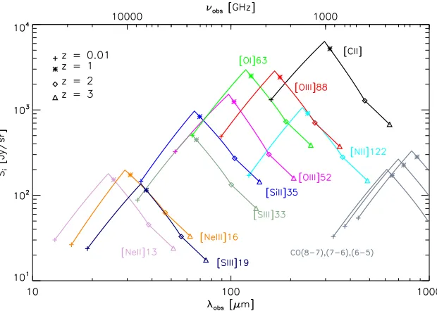
Figure 3: (left:) Infrared fine-structure line transitions frequently used in studies of the ISM. Lines are plotted as functions of their critical density and ionization energy, and are color-coded according to their application as diagnostics of regions of neutral and ionized gas: photodissoci-ation regions (green), stellar HII regions (red), active galactic nuclei (blue), and coronal regions (purple). Figure from Spinoglio et al. (2009). (right:) Sensitivity of the flux ratio of [OIII]88 µm to [NII]122µm emission to stellar temperature. Fluxes have been computed for plane-parallel HII region models using the publicly available radiative transfer codeCloudy(Ferland et al. 1998), and are presented as functions of the ionized gas density nH+ (units of cm−3) and the dimensionless
ionization parameter U, which specifies the ratio of the flux of ionizing photons to nH+. The
input ionizing spectra for the different HII region models are appropriate for stars with effective temperatures of 36000 K, 36300 K, 37000 K, 37300 K, and 48500 K. Note that the flux ratio is relatively independent of the ionized gas density, which is expected for a ratio of two ions with similar critical densities (cf. left panel of this Figure.)
wide range of environments throughout the star-forming medium, and result in the emission of IR photons—two facts which combine to position the IR FS lines as well-suited probes of galaxies during the epoch of peak cosmic SFR density. In fact, the IR FS lines are often the dominant coolants of the ionized and neutral atomic gas in galaxies, known collectively—along with molecular gas and a mixture of solids like dust and ice—as the interstellar medium (ISM); the total luminosity in a single FS line, such as the 158µm transition in the ground state of singly ionized carbon, can account for as much as 0.1–1% of a galaxy’s total IR luminosity.
conditions (e.g., density, flux of ionizing photons, dynamics, etc.) in a galaxy’s ISM is maximized by comparing observed fluxes in two or more lines in the form of flux ratios.
2PJ=1/2
2PJ=3/2
C+: 1s22s2 2p1
3PJ=0 3PJ=1 3PJ=2 1D
2 1S
0
O++: 1s22s2 2p2
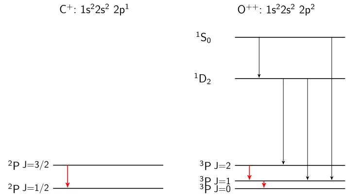
Figure 4: Schematic energy level diagrams for ground state electron configurations of singly ionized carbon, C+(left), and doubly ionized oxygen, O++(right). Energy levels are labeled using
the spectroscopic notation,2S+1L
J, whereS,L, andJ, refer to the spin, orbital, and total angular
momentum quantum numbers, respectively. Downward arrows indicate electronic transitions.
Important fine-structure transitions in the ISM of galaxies, namely, 2P
3/2 →2P1/2 for [CII] and 3P
1 →3P0 and 3P2 →3P1 for [OIII], are highlighted in red. These transitions correspond to
emission lines [CII]158µm, [OIII]88 µm, and [OIII]52µm, respectively.
Understanding the dependence of the intrinsic luminosity, Li, in a given line
transition i (or, equivalently, total gas cooling, Λi, in that transition) on various
physical properties of the emitting regions is essential to grasping how physical quantities are extracted from FS line ratio observations. Consider the ground state electronic configuration of singly ionized carbon, C+, which can be approximated as a two-level system (left panel of Figure 4) defined by its fine-structure. A downward electronic transition from the upper to the lower level (denoted as levels 2 and 1, re-spectively) results in the emission of an IR photon of wavelength 158µm, referred to as [CII]158µm9. As described in, for example, Tielens (2005) and Osterbrock (1989), in the optically thin limit—i.e., in the case where emitted photons escape the “par-ent cloud” without scattering or absorption, which is appropriate for [CII]158µm (and many of the IR FS lines, in fact) in most astrophysical conditions—it is possible to determine the relative population of each energy level in a straightforward way by assuming that the rate of downward and upward transitions between levels is in equilibrium and proceeds exclusively via collisional excitations and de-excitations
and spontaneous emission:
n1nγ12 | {z } upward transition
= n2nγ21+n2A21.
| {z }
downward transitions
(0.0.2)
In the above equation, A21 is the Einstein A coefficient for spontaneous emission (units of s−1) and n, n1, n2 refer to the number densities (units of cm−3) of the gas, and of carbon ions in levels 1 and 2. The coefficients γ12 and γ21 refer to the collisional excitation and de-excitation rates (units of cm3 s−1), respectively, which depend on the quantum mechanical collision strength of an atom or ion and (weakly) on temperature. Equation 0.0.2 can be re-written as
n2 n1
= nγ12
nγ21+ A21
. (0.0.3)
Based on the form of Equation 0.0.3, we consider two interesting limiting cases where we can calculate the line cooling rate, given by Λ[CII] =n2A21hν21, where h is Planck’s constant.
First, consider the low-density limit, where nγ21 A21. If we define a critical density, ncrit = A21/γ21, then this limit applies to all densities below the critical density, i.e., nncrit. Here, equation 0.0.3 simplifies to
n2 n1
= nγ12 A21
,
and the line cooling rate becomes
Λ[CII]=nn1γ12hν21, (0.0.4)
indicating that a photon is emitted for every collisional excitation in this case. Second, in the high-density limit, where nγ21A21 or nncrit, we have
n2 n1
= γ12
γ21
and
Λ[CII] =n1 γ12 γ21
A21hν21 (0.0.5)
Since the forms of the rate coefficients γ12 and γ21 are given explicitly as
γ12= βΩ12 g1T1/2
exp
−hν21
kBT
and γ21 = βΩ21 g2T1/2
, (0.0.6)
whereβ =h2/(k
level, and Ω12and Ω21 are quantum mechanical, dimensionless collisional strengths. Inserting the expressions for γ12 and γ21 in Equation 0.0.5, we find:
Λ[CII] =n1 g2Ω12 g1Ω21
exp
−hν21
kBT
A21hν21 (0.0.7)
which implies that, in the high-density limit, collisional excitations/de-excitations dominate and bring carbon ions to local thermal equilibrium with the collision part-ners (e.g., electrons), allowing the level populations to be given by the Boltzmann distribution at the kinetic temperature T.
The dependence of Λi on gas density is just one example of how properties of
the extragalactic ISM influence the observed emission in a given line transition. The line cooling rate also depends on many other properties of the ISM, such as the gas temperature relative to the separation between energy levels during the transition and the abundance of the emitting species, which is influenced by the metallicity of the gas, as well as the incident ionizing radiation on interstellar clouds. Thus, physical properties of the gas within galaxies can be difficult to extract from observation of individual emission lines. It is possible, however, to observe two or more emission lines in order to construct flux ratios in which various dependences on physical quantities are removed, leaving a dependence only a singly quantity to be measured. Observed flux ratios can be compared to their expected values from theory (e.g., Equations 0.0.4 and 0.0.7) in order to determine the prevalent physical properties of the ISM.
For example, the 52 µm and 88 µm transitions of doubly ionized oxygen (cf. Figure 4) are frequently used to determine the average density of ionized gas in galaxies. As they both arise from the same ion, these transitions are not dependent on the metallicity or ionization state of the gas. The fine structure levels involved in the transitions are also closely spaced in energy, so the transitions are also fairly insensitive to the gas temperature. With distinct critical densities ncrit= 500 cm−3
and 3,400 cm−3 for [OIII]88µm and [OIII]52µm, respectively, the corresponding flux ratio probes gas densities within the range defined by the different ncrit. When
n ncrit or n ncrit, the flux ratio is no longer dependent on gas density, but
on the ratio of statistical weights (for n ncrit) or the ratio of statistical weights
times A21 (for n ncrit), as demonstrated in Equations 0.0.4 and 0.0.7, albeit
modified for a three-level system appropriate for the oxygen transitions. Figure 1.8 in Chapter 1 shows the theoretical value of the [OIII]88µm and [OIII]52µm flux ratio as a function of ionized gas density.
The left panel of Figure 3 presents a set of IR FS lines that are commonly observed to originate throughout the ISM, and which are frequently used in the construction of so-called “diagnostic” line ratios. In this figure, FS lines are plotted as functions of their ionization energies (IEs) and the densities, ncrit, at which
flux ratios that probe the flux of Lyman continuum photons emitted from stellar populations and the gas density. Line ratios that are sensitive measures of gas density around star-forming regions, for example, include transitions from the same atom or ion, such as the 63µm and 146µm FS line transitions splitting the ground state of neutral oxygen, or the 52 µm and 88µm transitions of the doubly ionized atom, as discussed above. These transitions have the same elemental abundances (so they are not dependent on the metallicity or ionization state of the gas) and are very closely spaced in energy (so they are not sensitive to gas temperature), but they have distinct critical densities (so their flux ratio will be highly sensitive to the gas density). The ratio of the oxygen 88 µm line to the 122 µm line of singly ionized nitrogen, which have similar critical densities but different ionization energies, is another useful ratio, probing the effective temperature of stellar populations in DSFGs (right panel of Figure 3 by gauging the impingent ionizing flux. (Examples of other line ratios and their sensitivity to physical conditions in the ISM are compiled in Appendix A.) As illustrated in lefthand panel of Figure 3, ratios of FS lines can be used to probe a wide range of astrophysical environments.
In Chapter 1—a detailed study of the multi-component ISM in an AGN with ongoing SF during the epoch of peak cosmic SF—we make use of the IR FS lines of singly ionized carbon (158 µm line transition of [CII]), neutral oxygen (63 µm transition of [OI]), singly ionized nitrogen (122 µm transition of [NII]), and doubly ionized oxygen (52 µm transition of [OIII]). Because the epoch of peak galaxy cosmic SFR density also correlates with the epoch of peak supermassive black hole accretion rate density, the target of this study, called the Cloverleaf, is a well-suited laboratory to study the evolution of galaxies.
The ability to study the FS lines in distant galaxies on an object-by-object basis is challenged by a reduction in line flux by the factor (1 + z)2 due to the cosmological expansion, and so observing these lines in the Cloverleaf system at
z = 2.6 is partly enabled by its high intrinsic bolometric luminosity—nearly 1014 times the luminosity of the Sun, L—and an additional magnification from
gravita-tional lensing by foreground galaxies. Although galaxies with high IR luminosities called (ultra-)luminous infrared galaxies (LIR ≥ 1011 L) constitute the majority
extract-ing redshift-evolution in aggregate FS line luminosity density, and compares the effectiveness of traditional galaxy surveys to measure the same quantity (as well as to measure the power spectrum).
Chapter 1
Constraining ISM properties of
the Cloverleaf Quasar with
Herschel
spectroscopy
1.1
Introduction
Parallel histories of cosmic star formation (SF) and supermassive black hole (SMBH) accretion are suggestive of a causal relationship between the two processes, yet the nature of this link remains an open question in astrophysics. At the root of this connection is the cold molecular gas in galaxies, which must be shared as fuel for both growing black holes and budding stellar nurseries. Far from simple competitors, however, the roles of SF and SMBH growth in a galaxy’s evolution are varied and complex.(See, e.g., reviews on the subject by Heckman & Best (2014) and Madau & Dickinson (2014)). Molecular, star-forming gas in the circumnuclear region of galaxies known to host accreting SMBHs (called Active Galactic Nuclei, or AGN) are particularly useful test-beds for theories relating the feedback of the SMBH on SF (and vice versa) given the relatively short distances (∼1 kpc) between the molecular gas and the SMBH.
Figure 1.1
Figure 1.2: The Cloverleaf quasar imaged in three wavelengths. From left to right: optical (Hazard et al. 1984), millimeter (Alloin et al. 1997), far-infrared (Ferkinhoff et al. 2015).
stages of its longstanding role as a laboratory for high-z studies of molecular gas and SF in the environs of a powerful AGN. Since the first successful CO measurement, the Cloverleaf has been observed, to date, in numerous tracers of molecular gas, including 8 transitions of the CO ladder (J = 1 → 0 (Riechers et al. 2011a), 3 → 2 (Barvainis et al. 1997; Weiß et al. 2003), 4 → 3, 5 → 4 (Barvainis et al. 1997), 6 → 5 (Bradford et al. 2009a, hereafter B09), 7 → 6 (Alloin et al. 1997; Barvainis et al. 1997, B09), 8 → 7, and 9 → 8 (B09)), two fine-structure (FS) transitions of [CI] (3P
1 →3P0 (Weiß et al. 2005) and3P2 →3P1 (Weiß et al. 2003)), HCN (J = 1−0)(Solomon et al. 2003), and HCO+ (J = 1 → 0 (Riechers et al. 2006) and 4−3 (Riechers et al. 2011b)), and CN (Riechers et al. 2007). Spatial extent of the molecular gas, derived from a CO(J = 7 → 6) map, has also been assessed, and appears to be concentrated in a disk of radius 650 pc, centered on the SMBH (Venturini & Solomon 2003, VS03). Non-LTE modeling of CO excitation with an escape probability formalism suggests that all observed transitions can be described by a single gas component (Bradford et al. 2009a; Riechers et al. 2011a), so there is no indication of significant molecular emission in the observed lines beyond the CO(J = 7 → 6) disk. Physical conditions inferred from the modeling point to molecular gas densities of roughly nH2 = 2–3×10
4 cm−3 and high gas kinetic
temperatures of 50–60 K, suggesting that the CO gas is distributed uniformly or with high areal filling factors—not in sparse clumps—in order to maintain this thermal state throughout the ∼1 kpc-wide emitting region.
temperatures of ∼ 50 K and ∼ 115 K, respectively. The starburst origin of the cold gas component is strongly supported by the detection of emission features from polycyclic aromatic hydrocarbons (PAHs) in the Cloverleaf’s rest-frame mid-infrared spectrum, which were shown to follow the empirical correlation to FIR luminosity established for starbursts and composite quasar/starburst systems in the local Universe (Lutz et al. 2007). Attributing, then, the entirety of the FIR (42.5–122.5µm) luminosity, LFIR, inferred from the cold component of the SED, reveals a starburst of intrinsic LFIR = 5.4×10¹² L.
Identifying the dominant heating source of the molecular gas in the Cloverleaf is essential to understanding the relationship between the SMBH and SF in the host galaxy. In this paper, we present new measurements of key diagnostic lines of atomic and ionized media to aid in the interpretation of the excitation mechanisms for the observed CO in the Cloverleaf disk. The detected lines, namely [CII]158µm, [OI]63µm, [OIII]52µm, and [SiII]35µm, provide highly complementary information to the CO spectroscopy by tracing star-forming gas in different phases of the ISM, and by providing additional means to test XDR and PDR models, which can predict bright emission in the observed atomic lines.
This article is organized as follows. First, we report in Section 1.2 the measured line fluxes from Herschel-SPIRE and -PACS instruments, and discuss uncertainties where necessary. With observations of the important PDR cooling lines [CII]158µm and [OI]63µm enabled by Herschel, we are able to infer the average densities and FUV fluxes prevalent in the Cloverleaf PDRs by employing traditional FS line ratio diagnostics, as well as to better estimate the relative contribution of the AGN and SF to producing the observed emission, which we explore in Section 1.3. There, after subtracting contributions from ionized gas in the Narrow Line Region (NLR) and HII regions, we compare measured line ratios of the FS lines and CO to predicted values from PDR and XDR models and determine their respective contributions to the observed emission. We also briefly consider shock excitation of CO as an alternative explanation for the unusual high total CO line-to-FIR continuum ratio. Finally, in Section 1.4, we place our findings for the Cloverleaf in the context of other AGN discovered at similar and lower redshifts.
1.2
Observations
Measured fluxes for the fine-structure lines obtained in this work are presented in Table 1. We supplement our measurements with published fluxes for the [NII]122µm emission, CO up to J = 1–9, and the 6.2 µm and 7.7 µm PAH emission features.
the SPIRE Fourier Transform Spectrometer (SPIRE FTS) aboard Herschel. Point source spectra were obtained in sparse observing mode for the Cloverleaf with a total of 320 FTS scans—160 in each forward and reverse directions—from the Herschel
OT program OT1 mbradfor 1 (PI: Matt Bradford). Amounting to 364.4 minutes of observing time for the source, these spectra are the deepest SPIRE spectra yet presented, to our knowledge. The continuum level is at 0.1–0.5 Jy, which is close to the continuum flux accuracy achieved on SPIRE. As such, we take care to address concerns about spurious line detections arising from random noise fluctuations in the continuum, and—once lines have been identified—to accurately quantify uncer-tainties in the measured line fluxes.
To reduce the probability of a spurious line detection, we perform a jackknife test for each targeted line in which the full set of 320 unapodized spectra obtained from corresponding FTS scans is first split into two subsets. The jackknife split we apply is temporal, in order to test for variations in the spectrum as a function of observing time; we simply divide the scan set into halves containing scans 1–160 and 161–320, where scan 1 denotes the beginning of the observation and 320, the end. The 160 spectra in each half are then co-added to produce two separate spectra (called A and B), and then differenced to produce a residual spectrum. In the absence of systematic error between sets A and B, the differenced spectrum will contain zero flux at all wavelengths. Figure 1.3 shows the results of the jackknife tests for the [CII]158µm, [OI]µm63, and [OIII]88µm lines in 50 GHz1 segments centered at the rest wavelength for each line.
Line fluxes were measured from the unapodized spectrum using the Spectrum-Fitter in Herschel Interactive Processing Environment (HIPE) 12 version 1.0 (Ott 2010). We fit each emission line and 6 GHz of local continuum with a 1st order polynomial baseline and a Gaussian line profile convolved with a sinc function (i.e., “SincGauss” model in HIPE). Line centers, (1 +zClover)λrestwere fixed, as were the widths of the Gaussian and sinc profiles. The assumed Gaussian widths are not crucial to the fit—we adopted a FWHM of 500 km/s, on the upper range of that measured by Weiß et al. (2003) in the CO lines with the Plateau de Bure inter-ferometer. For the sinc function, we fixed the width at 0.38 GHz, which is set by the spectral resolution of the FTS (in high resolution mode). The SpectrumFitter returns the fitted parameters for the SincGauss model, which we convert to flux using the appropriate analytic formula. It also provides an associated uncertainty, which we consider as a lower limit. We proceed to generate our own estimate of the RMS noise in 50 GHz of bandwidth centered at the target frequency. In our estimate, we repeatedly fit our SincGauss model at various frequencies within this bandwidth. Because the SPIRE FTS has a spectral resolution of 1.2 GHz, there are 41 independently sampled frequencies—and thus 41 independent line flux fits—in each 50 GHz range. The uncertainty reported in Table 1.1 is the standard deviation (equal to the RMS for the zero-mean signal) of the sampled frequencies, plus a 5%
calibration uncertainty for SPIRE. A histogram of the flux fits using our uncer-tainty estimate is displayed in the righthand panels of Figure 1.3. Note that the histograms are centered at zero, as expected for random noise. For reference, the measured flux of the target line is also shown (dashed vertical line) in the histogram plot, and is given in Table 1.1. The lines [CII]158µm and [OI]63µm are detected at levels of 3.8σ and 8.5σ, respectively. A 2σ upper limit is reported for [OIII]88µm.
PACS Point-source observations of the Cloverleaf include spectra from the blue and red channels, which cover the wavelength range corresponding to expected FS line emission from [OIII]52µm, [SiII]35µm, [SIII]33µm, [FeII]26µm, and [OIV]26µm. Spectra for [OIII]52µm and [SiII]35µm were obtained from theOT1 mbradfor 1 ob-serving program; [OIII]52µm, [SIII]33µm, [FeII]26µm, and [OIV]26µm spectra were obtained from the Key Program KPGT kmeisenh 1 (PI: Klaus Meisenheimer). The two spectra containing the [OIII]52µm line were co-added using the AverageSpectra task in HIPE. The data were reduced with the background normalization version of the chopped line scan reduction script included in HIPE. We reduced the data with
oversample= 4, then binned by a factor of 2 in post-processing to achieve Nyquist sampling. Processed spectra with error bars and line fits (blue curves) for the targeted lines are presented in Figure 1.4. Measured fluxes and uncertainties (ob-tained directly from SpectrumFitter) are listed in Table 1.1. While we only report detections for [OIII]52µm (5.1σ) and [SiII]µm (7.8σ), an upper limit for [OIV]26µm is also given, and we include spectra of the other lines (namely, [FeII]26µm and [SIII]33µm) for completeness.
1.2.1
Extinction corrections
While the far-IR lines are relatively extinction-free, corrections are required for the most highly-obscured systems. In Arp 220, for example, Rangwala et al. (2011) find that the dust is optically thick at 240µm, corresponding to a column density in hydrogen, NH, of 1025cm−2. This extreme source demands corrections even for the submillimeter mid-J CO transitions.
The Cloverleaf has similar gas and dust masses to Arp 220, but the extinction is reduced because the size scale is larger. We estimate extinction values using both gas and dust mass, in both cases spread over the 650-pc radius disk (including the 30◦ inclination), with an area of 1.1×1043cm2. For the gas mass, we take the peak of the B09 molecular gas mass likelihood of 6×10⁹M, which corresponds
to a typical hydrogen column in the disk of 4.7×1023cm−2. Per the mixed-dust model of Li & Draine (2001), this column creates 0.8 magnitudes of extinction at 63µm, corresponding to an optical depth,τ, of 0.73; and, the model predicts a ν−2
scaling with τ for wavelengths between 30µm and 1000m. A similar estimate is obtained with the estimated dust mass from Weiß et al. (2003), some 6.1×10⁷M
.
absorption coefficient in Table 6 of Li & Draine (2001)—adjusted to 63 microns— givesκ63= 84.7 cm2g−1, and an optical depth of 0.93. We adopt the average of these values (τ63 = 0.83), and use a mixed dust extinction model in which the correction factor relating observed to intrinsic flux is τd/(1−e−τd). The mixed-dust model
is appropriate if the emission lines originate in gas mixed approximately uniformly with the disk, as is the basic scenario for the star-forming disk material. For emission from the AGN narrow-line region (NLR), the correction could potentially be greater if the NLR gas is fully covered by the disk. On the other hand, at least some portion of the NLR material is largely unobscured, since NLR gas is visible at optical wavelengths. Given these uncertainties, the modest correction of the mixed dust model seems appropriate. The correction factor for [OI]63 is 1.47, and the other transitions are corrected similarly assuming τ ∝ ν−2. Line fluxes reddened according the necessary correction factors are listed in Table 1.1.
1.3
Analysis
In this section, we use the suite of CO rotational transitions (from the literature), the [NII]122µm line (Ferkinhoff et al. 2011a, F11), and the newly detected (>3.5σ) atomic FS lines (from this work) in diagnosing the physical conditions prevalent in the ISM of the Cloverleaf system.
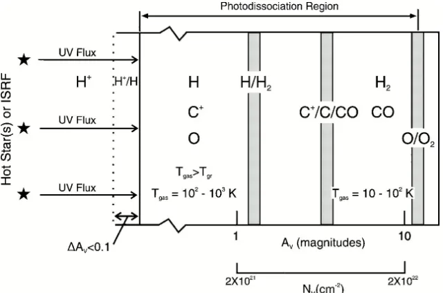
Although the dataset of detected lines is rich, the natural complexities of a multiphase ISM must be treated carefully, particularly given that many of the observed transitions can be excited in a variety of physical environments: photon-dominated regions (PDRs), dense stellar HII regions, diffuse ionized gas, the clouds of the NLR near the AGN, or X-ray Dominated Regions (XDRs); see Figure 1.5 for a cartoon representation of the various ISM phases and the corresponding emission lines expected from each phase. High resolution spatio-spectral imaging data for the set of observed emission lines is limited, but is helpful in partitioning ISM components when available, as in the case of CO(J = 7 → 6) and [NII]122µm. The FS line observations presented here are all spatially unresolved; the smallest beam sizes for Herschel-SPIRE and -PACS imaging spectrometers are 17” and 9”,
respectively, compared to the on-sky diameter of 2” for the optical quasar and the interferometric CO(J = 7 → 6) image. We are therefore considering integrated emission from the composite source and begin by considering how the atomic line emission is partitioned among the various components.
1.3.1
[CII]158
µ
m from non-star-forming gas
The optically thin [CII]158µm emission can be used to assess the mass of [CII]158µ m-emitting atomic gas,MH, by comparing the measured [CII]158µm luminosity,L[CII], to the expected C+ cooling rate (units of erg s−1 per H atom). Following Hailey-Dunsheath et al. (2010b) (cf. their Equation 1), and using the PDR surface tem-perature TPDR ∼ 300 K and density nH = 3.16×103 cm−3—see Section 1.3.2 for justification of TPDR and nH adopted here—we findMH∼2×10¹⁰ M. This value
is on the high end of the Cloverleaf’s molecular gas mass estimated by B09 (MH2 ∼
0.3–3×10¹⁰M
), indicating that the mass in PDRs comprises a substantial fraction
of the total gas mass in the ISM.
With a first ionization energy (IE = 11.26 eV) lying just below 1 Rydberg, singly-ionized carbon can coexist with both neutral and singly-ionized hydrogen. Thus, while we expect that PDRs illuminated by star-formation may be the dominant source of [CII]158µm emission, we must consider stellar HII regions (denoted in symbols with subscripts as “HII?” throughout this article) and the AGN-ionized NLR, as well.
The sum of each ISM phase’s contribution—expressed as the fraction, α[CII],j, of
observed flux for [CII]158µm (or generally any linei) and ISM phasej—will sum to the measured total line flux, F[CII], so that the flux attributed to PDRs, F[CII],PDR, is written as
F[CII],PDR = (1−α[CII],NLR−α[CII],HII?)×F[CII] (1.3.1)
We note that F11 measured the total [NII]122µm luminosity, L[NII]122, in the Cloverleaf, and placed a lower limit on the mass of ionized gas,MH+ ∼2.1×10⁹ M,
by calculating the N+ cooling rate for high ionized gas densities (n
H+ ncrit,e−)
and temperatures at which all nitrogen exists in the singly-ionized state. Working in the same high-density, high-temperature limit, we estimate the minimum expected luminosity of [CII]158µm from their inferred ionized gas mass as ∼2×10⁹ L
, or,
roughly &10% of L[CII].
Narrow Line Region As the AGN is responsible for roughly 90% of the Clover-leaf’s bolometric luminosity, we first consider the potential for [CII]158µm emission arising in the NLR associated with the immediate vicinity (of the order 10–100 pc) of the central accretion zone.
dish in F11, and is coincident with the quasar point source. Since the line is spatially unresolved with a synthesized beam size of ∼ 0.25” (or ∼ 180 pc in the source plane), they concluded that the detected emission can be ascribed to the NLR, while the undetected flux originates from a more extended area and has thus been “resolved out” by the small ALMA beam. We use this upper limit to estimate, based on theoretical models, the corresponding [CII]158µm emission for given physical conditions prevalent in the NLR by writing
α[CII],NLR =
γ[CII],NLR(G04) ×F[NII]122,NLR
F[CII]
(1.3.2)
where F[NII]122,NLR (= 0.2F[NII]122) is the observed NLR flux of the [NII]122µm line based on the ALMA observation. The factor γ[CII],NLR(G04) is, explicitly, written as
γ[CII],NLR(G04) = F (G04) [CII],NLR
F[NII]122,NLR(G04) ,
representing the scaling between the predicted fluxes of [CII]158µm and [NII]122µm—
F[CII],NLR(G04) and F[NII]122,NLR(G04) , respectively—from a NLR theoretical model, namely, that of Groves et al. (2004, G04). We correct carbon and nitrogen abundances from solar values of adopted in G04 to match ISM values that we later use when considering the stellar HII region contribution to [CII]158µm; the ISM abundance set adopts a nitrogen abundance that is a factor of 1.3 greater than specified by the solar abundance set in G04.
Output of the G04 NLR models can be parametrized on grids of nH and a dimensionless ionization parameter, U = (ΦLyC)/(nHc), where ΦLyC is the rate of Lyman continuum photons per unit area from the AGN incident on the cloud surface, and cis the speed of light. According to these grids, γ[CII],NLR(G04) is relatively
insensitive to U andnH, so thatγ[CII],NLR(G04) = 4.6–7.7 throughout the parameter space for models with intrinsic power-law ionizing continua with spectral indices of -1.7 or -2.0. Adopting this range of γ[CII],NLR, we place an upper bound on the fraction of flux of [CII]158µm emerging from the NLR asα[CII]158,NLR ≤ 0.15–0.25.
1.3.2
Star-forming ISM: PDRs and stellar HII regions
PDR diagnostics Photon dominated regions (PDRs) are broadly defined as re-gions of the neutral ISM where photons with energies, Eγ, in the far-ultraviolet
regime (6 eV < Eγ < 13.6 eV) are responsible for driving the local chemical and
Figure 1.6: Schematic of PDR structure. Figure from Hollenbach & Tielens (1997).
represented as a uniform density slab, the warm surface layers (AV ≤ 1−4) are
composed primarily of hydrogen and oxygen in their atomic forms, and singly ion-ized carbon. [CII] and [OI]63 emission primarily originate from this zone. Beyond
AV ' 4, which is a couple of magnitudes of visual extinction past the transition
from atomic to molecular hydrogen, neutral oxygen persists, but carbon is no longer ionized. Instead, carbon recombines to form CO, and CO cooling dominates at these cloud depths.
Plane-parallel, semi-infinite slab models (e.g., Kaufman et al. (2006); K06) devel-oped exclusively for PDRs can determine cloud structure and predict the emergent intensity of both lines and continuum emission by internally solving radiative trans-fer and thermal and chemical balance of the cloud with two parameters: incident FUV flux, G02, and cloud density, nH =nH0 +nH
2. The freedom to tune G0 and nH over a wide range of values is an appealing feature of these models, permitting them to describe emission from a correspondingly wide range of physical conditions, and thus extending PDR predictions beyond the interpretation of photodissociation regions as existing exclusively between HII regions and molecular clouds.
The [OI]63 and [CII] lines are theoretically and empirically the dominant cooling lines in PDRs. The [OI]63 line lies much higher above the ground state than the [CII] line—228 K vs 92 K—and has a much higher critical density—3×105 cm−3 vs 3×103 cm−3. Hence, [OI]63 emission is favored when the impinging FUV radiation (and thus gas temperature) and gas density are both high, and the flux ratio of these lines is a useful diagnostic of incident FUV flux and density. With disparate
2G
0 is normalized to the average value in the plane of the Milky Way, such that G0 = 1
critical densities and energies above ground, their flux ratio F[OI]63
F[CII] is a useful probe
of the gas density and average FUV field. Similarly, F[CII]+F[OI]63
FFIR is another
diagnos-tic ratio of PDR density and the impingent FUV radiation field, as this ratio of flux from from cooling lines relative to thermal dust emission essentially represents the photoelectric heating efficiency of the dust grains, which is determined by G0/nH. In this way, [CII] and [OI]63, along with the FIR continuum, have been used ex-tensively as probes of the physical conditions in PDRs, often being presented in so-called “PDR diagnostic diagrams,” wherein the observed values of line ratios are plotted as functions of G0 and nH.
To understand the star-forming ISM, we begin by incorporating the [CII]158µm and [OI]63µm fluxes, as well as the far-IR continuum, in the commonly-used frame-work of the PDR diagnostic diagram in Figure A.13. Here we assume that all of the measured FIR luminosity is generated from the starburst component in Cloverleaf, with negligible contamination from the AGN, as discussed in Lutz et al. (2007). According to Figure A.13, PDR models with nH ∼ 2–6×103 cm−3 and G0 ∼ 3– 7×10²can generate line ratios that are compatible with observations when assuming Fi,PDR =Fi; the parameters nH= 3.16×103 cm−3 and G0 = 3.16×10² correspond to the PDR model with the lowest value of the χ2 statistic. Note that we have not yet made any allowances for a possible contribution of observed [CII]158µm and [OI]63µm emission from ISM components distinct from PDRs. The only ad-justment has been to double the measured [OI]63µm flux, as per Kaufman et al. (1999), before comparing measurements to theoretical predictions from K06. This correction is necessary because, while the intensities computed for the PDR models emerge from a single, illuminated face, the geometry of emitting regions in Clover-leaf is assumed to be such that individual PDRs are illuminated by FUV photons on all sides; optically thick [OI]63µm line emission emerging from cloud surfaces opposite the observer will not contribute to the measured flux.
Stellar HII regions We can constrain α[CII],HII? in Equation 1.3.1 using the [NII]122µm flux measured in F11. With similar ionization potentials, singly-ionized nitrogen is often found in the same ionized gas as singly ionized carbon. Its slightly higher first ionization energy (IE = 14.5 eV), however, prevents the nitrogen ions from forming in neutral gas. Thus, identifying an excess in the measured flux ratio,
Figure 1.7: PDR diagnostic plots. Left panel: Red and blue curves denote observed values (solid) and associated uncertainties (dotted) of flux ratios F[OI]/F[CII] and F[OI]+F[CII]
/FFIR,
respectively. The filled black star symbol indicates the corresponding PDR solution innHandG0,
which refers to the PDR model with minimumχ2. The un-filled star represents the PDR solution
with F[CII],PDR = 0.6F[CII], i.e., after applying corrections for NLR and HII region contributions
to the measured [CII]158µm flux. The confidence region within one standard deviation from each PDR solution is outlined by black dotted contours. Black dashed contours represent thermal pressure at the PDR surface. Right panel: Observed CO line flux ratios are shown along with the FS line ratios. The cyan curve shows FCO(J=7→6)/FCO(J=2→1). Thick and thin magenta curves
correspond to the observed and theoretical values, respectively, of FCO(J=7→6)/FFIR. Vectors
indicate the direction and magnitude of change in the PDR solution located atnH= 3, 160 cm−3
andG0= 316, when altering the PDR contribution to [OI]63µm and [CII]158µm flux. Percentages
photo-ionization code Cloudy3 (Ferland et al. 1998, version 10.0); the theoretical ratio, F[CII],HII(Cloudy)?/F
(Cloudy)
[NII]122,HII?, is shown in Figure 1.8 as functions of U and nH+. It
Figure 1.8: Theoretical line flux ratios F[CII],HII(Cloudy)?/F
(Cloudy)
[NII]122,HII? and F
(Cloudy)
[OIII]88,HII?/F
(Cloudy)
[OIII]52,HII?
(red and blue curves, respectively) as a function of ionized gas density and computed for different ionization parameters (U = −4.0, dashed curves; U = −1.0, solid curves), computed for the HII region only. Magenta and cyan horizontal lines denote the measured value and upper limit of the respective ratios in the Cloverleaf. Measured fluxes of [CII]158µm and [NII]122µm have been corrected for NLR contributions according to α[CII],NLR ≤ 0.2 and α[NII]122,NLR ≤ 0.2,
as discussed in Section 1.3.1. Error bar indicates the range of uncertainty in the ratio after propagating uncertainties on the [CII]158µm and [NII]122µm fluxes. Downward pointing arrows indicate that the [OIII]88µm/[OIII]52µm ratio represents an upper limit, having used the 2σupper limit reported for [OIII]88µm.
is clear that the contribution of [CII]158µm from ionized gas can be large for low densities (nH+ < 10 cm−3) and low ionization parameters (U ∼ 10−4). Note that
the common ionized gas density probe, the [OIII]88µm-to-[OIII]52µm flux ratio
F[OIII]88,HII(Cloudy) ?/F
(Cloudy)
[OIII]52,HII?, is predicted to be less than 1.8 for all considered densities, 1 cm−3< nH+ <104 cm−3. This value is below the ratio (<2.3) derived from the
upper limit on F[OIII]88 and the detection of F[OIII]52, so we must use an alternative means of estimating an average gas density in the Cloverleaf’s stellar HII regions. If we assume that the HII regions are physically adjoined to PDRs, then we can impose thermal pressure equilibrium at the boundary between the two ISM phases, and rule out nH+ .10 cm−3, since these diffuse HII regions have thermal pressures, Pth/kB, in the range of ∼104–105 K cm−3, as calculated internally byCloudy; such
3We have used a plane-parallel geometry with ionizing spectrum from CoStar stellar
thermal pressures are too low to be in equilibrium with the K06 PDR models, which have at least 106 cm−3 K. In fact, the pressure in the PDR increases when the PDR contribution of [CII]158µm is reduced, leading to more tension with very low den-sity HII region models. Pressure-matching4 with the K06 PDRs favors HII region models with nH+ = 0.56–3.2×102 cm−3, corresponding to α[CII],HII? = 0.23–0.08.
While pressure equilibrium between the HII regions and PDRs may be an overly idealized assumption, observations in star-forming regions, individual galaxies, and statistical samples of galaxies (cf. Oberst et al. (2006), Rangwala et al. (2011), and Vasta et al. (2010) for examples of each) indicate α[CII],HII? <0.3. Thus, we adopt the upper value derived from the pressure-matched solution, α[CII],HII? = 0.2, and correspondingly subtract the HII region component from the measured flux. We find that the corrected diagnostic ratios favor nH= 5.6×103 cm−3 and G0 = 5.6×10². If we correct F[CII] with the combined contributions from the NLR and HII regions, as in Equation 1.3.1, we find that the only change in the preferred PDR solution is an increase in G0 to 103.
Geometric considerations
Following Stacey et al. (2010a) and authors thereafter, it is useful to compare the value of G0 predicted from the PDR models with the value estimated solely from geometric considerations. As described in Wolfire et al. (1990), if PDR surfaces and the sources of radiation are randomly distributed—such as in the case of stel-lar populations—within a region of diameter D, then the photons in this region will likely be absorbed by a PDR cloud before traveling a distance D so that the impingent FUV flux on cloud surfaces in the emitting region is simply related to the surrounding volume density of FUV photons, G0 ∝ (λLFIR)/D3, where λ is the mean-free path of FUV photons. However, if FUV photons can travel large distances (compared to D) until being absorbed, then the FUV flux will vary as the surface flux of FUV photons, G0 ∝ LFIR/D2. The constants of proportionality can be determined by calibrating to known values5 of G
0, LFIR, andD for M82 (as in, for example, Stacey et al. (2010a)). These two scenarios, set apart by different assumptions regarding λ, represent limiting cases for which we can calculate the expected G0, givenD and LFIR for the Cloverleaf.
To make this comparison, we adopt the source size inferred from gravitational lens modeling (VS03) of spatially resolved CO(7-6) flux, implicitly assuming that the CO(7-6) line emission is co-spatial with the FIR continuum. For the Cloverleaf, there exists spatially resolved continuum data (F15) in the rest-frame FIR (122µm) that would—barring significant contribution at this wavelength from the AGN as
4Given the discrepancies in the internal radiative transfer, adopted microphysics, etc., we
consider pressures between the HII region and the PDR models to be in equilibrium as long as the values agree within a factor of 2.
5For M82,G
0= 102.8 andLFIR= 3.2×10¹⁰(Colbert et al. 1999a), andD= 300 pc (Joy et al.
inferred from the double-peaked SED in Weiß et al. (2003)— enable a direct mea-surement of the extent of the FIR-emitting region in the context of a gravitational lens model that relates the observed surface brightness distribution to a physical size in the source plane. A comparison between the 122µm continuum and CO(7-6) maps shows that the two tracers peak at the same locations the four lensed quasar images, supporting our claim that the two emission regions overlap. Setting
D = 1.3 kpc, then, we estimate G0 ∼ 1.3–5.7×10³ using the two relations with different assumptions about the mean-free path of FUV photons in the Cloverleaf disk.
This inferred G0 value is above the range predicted by the PDR diagnostic line ratios when assuming all observed [CII]158µm and [OI]63µm is produced in PDRs. Broadly, larger values of F[OI],PDR/F[CII],PDR tend to implicate higher values of G0. It is important to note that we do not consider increasing the [OI]63µm flux beyond the extinction and optical depth correction factors already discussed, as there is no evidence of self-absorption in the spectrally resolved [OI]63µm line profile. Simultaneous decreases in F[OI],PDR and F[CII],PDR, which increases the FIR continuum flux relative to the total FS line cooling, points to higher G0, as well (cf. Figure A.13). The effects on the derived PDR parameters of reducing the PDR contribution of [CII]158µm while keeping the [OI]63µm flux constant, of reducing the PDR contribution while keeping the [CII]158µm flux fixed, and of decreasing by equal amounts the PDR contributions of [OI]63µm and [CII]158µm are illustrated by vectors drawn in the righthand panel of Figure A.13.
CO from PDR models
![Figure 1.3:SPIRE FTS spectra for [CII]158vertical lines denote the fitted flux at the target line center for the coadded spectrum and thepanels)](https://thumb-us.123doks.com/thumbv2/123dok_us/9355827.1469607/27.612.123.537.114.528/figure-spectra-vertical-denote-tted-coadded-spectrum-thepanels.webp)
![Figure 1.4:Resampled continuum-subtracted PACS spectra with error bars for [OIII]52[SIII]33width) for spectral lines are shown as blue curves](https://thumb-us.123doks.com/thumbv2/123dok_us/9355827.1469607/28.612.149.499.213.488/figure-resampled-continuum-subtracted-pacs-spectra-spectral-curves.webp)
![Figure 1.8: Theoretical line flux ratiosindicate that the [OIII]88limit reported for [OIII]88 F (Cloudy)[CII],HII⋆/F (Cloudy)[NII]122,HII⋆ and F (Cloudy)[OIII]88,HII⋆/F (Cloudy)[OIII]52,HII⋆(red and blue curves, respectively) as a function of ionized gas de](https://thumb-us.123doks.com/thumbv2/123dok_us/9355827.1469607/35.612.164.479.125.340/figure-theoretical-ratiosindicate-reported-cloudy-cloudy-respectively-function.webp)