www.nat-hazards-earth-syst-sci.net/10/149/2010/ © Author(s) 2010. This work is distributed under the Creative Commons Attribution 3.0 License.
and Earth
System Sciences
Time-dependent
Z
-
R
relationships for estimating rainfall fields
from radar measurements
L. Alfieri1,2, P. Claps1, and F. Laio1
1Dipartimento di Idraulica, Trasporti ed Infrastrutture Civili (DITIC), Politecnico di Torino, Torino, Italy 2Institute for Environment and Sustainability (IES), Joint Research Centre, EC, Ispra, Italy
Received: 26 March 2008 – Revised: 29 October 2009 – Accepted: 22 December 2009 – Published: 26 January 2010
Abstract. The operational use of weather radars has become a widespread and useful tool for estimating rainfall fields. The radar-gauge adjustment is a commonly adopted tech-nique which allows one to reduce bias and dispersion be-tween radar rainfall estimates and the corresponding ground measurements provided by rain gauges.
This paper investigates a new methodology for estimating radar-based rainfall fields by recalibrating at each time step the reflectivity-rainfall rate (Z-R) relationship on the basis of ground measurements provided by a rain gauge network. The power-law equation for converting reflectivity measure-ments into rainfall rates is readjusted at each time step, by calibrating its parameters using hourlyZ-R pairs collected in the proximity of the considered time step. Calibration windows with duration between 1 and 24 h are used for esti-mating the parameters of theZ-Rrelationship. A case study pertaining to 19 rainfall events occurred in the north-western Italy is considered, in an area located within 25 km from the radar site, with available measurements of rainfall rate at the ground and radar reflectivity aloft. Results obtained with the proposed method are compared to those of three other liter-ature methods. Applications are described for a posteriori evaluation of rainfall fields and for real-time estimation. Re-sults suggest that the use of a calibration window of 2–5 h yields the best performances, with improvements that reach the 28% of the standard error obtained by using the most ac-curate fixed (climatological)Z-Rrelationship.
1 Introduction
Advances achieved in the recent past in radar technology and in the methods for processing data are leading to an in-creasing confidence toward the use of radar-based rainfall
Correspondence to: L. Alfieri
estimates into hydrologic analyses and simulations. An accu-rate knowledge of the spatial characteristics and the amount of rainfall falling on a catchment area is of crucial impor-tance in flood forecasting and warning systems (Smith, 1993; Claps and Siccardi, 1999; Arnaud et al., 2002; Brath et al., 2004), and can substantially improve the allocation of wa-ter resources for agricultural uses as well as for hydroelec-tric production (Alfieri et al., 2006). Further, an accurate quantitative precipitation estimation through radar measure-ments can provide an aid to the understanding of relations between point and areal rainfall (Bacchi and Ranzi, 1996) and for defining the probability distribution of annual rain-fall intensity for large return periods (i.e., high rainrain-fall rates), due to the large amount of data that the radar collects at each scan (e.g., Koistinen et al., 2006).
Woodley et al. (1975), among others. However, because of the considerable variability that the raindrop size distribu-tion shows during a rainfall event, the actualZ-R relation changes continuously in space and time. Therefore, the ma-jor drawback of using a unique relationship is that it can-not account for the broad variability of the trueZ-R rela-tion in the presence of different types of precipitarela-tion (e.g., convective or stratiform), as well as the variations that oc-cur within each rainfall event (e.g., see Richards and Crozier, 1983; Smith and Krajewski, 1993; Lee and Zawadzki, 2005). Several approaches for improving the radar estimates of rainfall based on radar-gauge comparisons have been pro-posed in the past years (e.g., Brandes, 1975; Zawadzki, 1975; Collier et al., 1983; Austin, 1987; Ulbrich and Lee, 1999). These methods often try to reduce the estimation uncertainty by introducing additional information such as the precipita-tion type (e.g., convective or stratiform), the distance of the gauge from the radar, the elevation of the radar beam, and so forth (see for example Joss and Lee, 1995; Anagnostou and Krajewski, 1999a, b; Gabella and Amitai, 2000). Recent applications of real-time procedures are reported in Seo and Breidenbach (2002), Chumchean et al. (2006), Germann et al. (2006), Chiang et al. (2007).
Legates (2000) carried out a real-time calibration of the Z-Rpower-law relationship by considering the radar-gauge pairs of the previous month characterized by non-zero rain-fall, in order to account for seasonal fluctuations due to dif-ferent types of precipitation and for possible drifts of the hardware calibration. It is known that the actualZ-R rela-tion is subject to variarela-tions on much shorter time scales, but it is still not clear whether an optimal calibration period for providing the best rainfall estimates is definable.
In the present paper, we propose a simple methodology for producing accurate radar-based estimates of rainfall in-tensity, by readjusting the coefficients of theZ-R relation-ship continuously in time considering short calibration win-dows. The procedure is tested on 19 rainfall events, with no recorded snow on the ground, that occurred in the north-western Italy between 2003 and 2006. We use reflectivity measurements from a weather radar and rainfall data from a network of 20 rain gauges located within a range of 25 km from the radar.
The next section describes the procedure devised for esti-mating rainfall fields from radar-gauge pairs. Section 3 gives some information on the case study and the data adopted; then it shows the results obtained with the two proposed tech-niques and a comparison with those of some literature meth-ods. Some conclusions are reported in the final section. 2 Methods
The basic idea behind this work is that, for each time stept, one can estimate as manyZ-Rrelationships as the number of the available data pairs in theZ-Rplane. When a
two-para-meters power-law of the form
Z=a·Rb (1)
is adopted, the coefficients a and b can be obtained by fitting the relation to match at least two points identified by non-zero concurrent measurements of rainfall rate and radar reflectivity. The Z-R pairs can be taken either at the same spatial coordinates (i.e., the same rain gauge j) at different times (i.e., {Z1=Z (ti,j ),R1=R (ti,j )} and {Z2=Z (ti+1,j ),R2=R (ti+1,j )}), or for the
same time step ti, considering two neighboring rain gauges (i.e., {Z1=Z(ti,j ),R1=R(ti,j )} and
{Z2=Z (ti,j+1),R2=R (ti,j+1)}), where it is con-ventionally assumed thatj+1 is the rain gauge closest to j. If the measurements were not affected by errors, for (ti+1−ti) approaching zero (or for the distance betweenj andj+1 approaching zero) the relation obtained by using only two Z-R pairs would be the most suitable to convert reflectivity measurements in rainfall rates. Of course, the relation would change when moving to a different place or considering another instant in time.
The above described procedure is not practicable, due to a number of limitations which affect the problem. First, the radar reflectivity and the ground-rainfall measurements are subject to several sources of error (e.g., see Steiner et al., 1999). As a consequence, the adoption of only two Z-R pairs for estimating the coefficientsa andb would provide scarcely-reliable and highly fickle relationships. A further major source of uncertainty is due to the non-homogeneity of the volume sampled by the two instruments and to a possible temporal lag between the two measured variables (e.g., Za-wadzki, 1975). The radar carries out instantaneous measure-ments of volume aloft, whose size varies with the distance from the radar. The rain gauges that we considered measure cumulative rainfall depths at the ground level, by sampling an area of 200 cm2 for a duration as long as the sampling time (10 min for this study).
Because of the difficulty to defineZ-Rpairs which refer to the same volume of atmosphere sampled, rainfall measure-ments are usually aggregated over longer durations. Like-wise, radar data are averaged over time and space, by con-sidering a number of pixels from the reflectivity maps nearby the position of the rain gauges and a duration corresponding to the same one adopted for the rainfall data aggregation. In this work, the choice of the aggregation period is one hour in time and nine radar pixels in space (i.e. a 1.5×1.5 km2 area) centered on the pixel which contains the considered rain gauge.
d, taken in the proximity of the selected instantti. As a con-sequence, each power-law regression is carried out on a num-ber ofZ-Rpairs with an upper boundNRG·d, given by the
number of rain gaugesNRGtimes the durationd(in hours) of
the calibration window. Different calibration windows of du-rations between 1 and 24 h are tested, and results are shown and discussed in Sect. 3.2 and 3.3. Parameters of each power-law relationship are calculated by minimizing the squared differences between the observed and the estimated rainfall values. The latter are obtained through
R=10∧
Z∗
10bˆ
−logaˆ ˆ
b
, (2)
whereaˆ andbˆare the coefficients to estimate. Equation (2) is obtained from Eq. (1), by considering that the reflectiv-ity data are provided in the formZ∗=10 log Z [dBZ]. Note that, despite Eq. (2) represents a straight line in the bi-logarithmic plane log Z-logR, the regression procedure is carried out in theZ-R plane by means of non-linear tech-niques. The adopted optimization algorithm is a subspace trust region method and is based on the interior-reflective Newton method. The optimized coefficientsaˆ andbˆare es-timated iteratively by taking those obtained from the linear regression method (see Eq. 3) as first attempt values. The non-linear optimization causes a substantial heteroscedastic-ity of the estimation residuals, but it is necessary for obtain-ing regressions producobtain-ing small errors also at high rainfall intensities, which is important when dealing with extreme precipitation events. Further, this approach has the advan-tage of producing almost unchangedZ-Rrelationships when a threshold for the minimum considered value of reflectivity is set. This is better clarified at the end of this section.
In order to assess the performances of the mentioned non-linear regression method we carried out a comparison of the results obtained with this method and with the commonly adopted method based on the equation
logZ=logaˆ0+ ˆb0logR, (3)
derived from Eq. (1), whereaˆ0andbˆ0are the estimated val-ues ofa andb. Results of such comparison are discussed in Sect. 3.2.
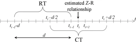
The calibration procedure was then used both for (i) a pos-teriori evaluation of the rainfall field, hereafter referred to as “continuous-time” (CT) readjustment, and (ii) for real-time (RT) estimation. In the first case, for each time stepti, the Z-Rrelationship is estimated by considering theZ-R pairs for a time window of durationdcentered onti, i.e., taking all the available pairs betweenti−d/2 andti+d/2. In real-time monitoring the aim is to estimate the current rainfall field from reflectivity measurements at the same instantti, where each relation is estimated from theZ-Rpairs of the preced-ing hours. In this case the relation to use at the timeti was inferred from theZ-Rpairs betweenti−1−d andti−1.
Fig-ure 1 shows a scheme of the calibration windows to assume
Fig. 1. Calibration windows considered for estimating theZ-R re-lationship at a given time stepti. Both windows for real-time (RT) estimation and continuous-time (CT) readjustment are shown.
(both for CT readjustment and RT estimations) for a certain durationd and time stepti, wheret andd are expressed in hours.
Some further details are needed to clarify the operational use of the method. For some time windows no validZ-R relationship was found, either because fewZ-R pairs were available for the corresponding calibration window (i.e., rain-fall was zero for most of the rain gauges) or because the co-efficients of the power-law did not comply with the imposed constraints,a >1 andˆ b >1. We rejected the estimatedˆ Z-R relationships characterized by coefficientsa <1 orˆ b <1, inˆ that they produce unreliable estimates of the rainfall rate for large values of the reflectivity. A physical interpretation of the assumptionb >1 was also suggested by Smith and Kra-ˆ jewski (1993), who considered the effect of the variability of the raindrop characteristics within a statistical model for estimating the power-law parameters.
For these cases the relation to adopt was chosen as the closest one in time. In particular, for CT estimation, when the calibration window [ti−d/2, ti+d/2] does not provide a valid relationship, the windows [ti+1−d/2, ti+1+d/2],
[ti−1−d/2,ti−1+d/2], [ti+2−d/2, ti+2+d/2], [ti−2−d/2,
ti−2+d/2] and so forth, are tested progressively until the first
relationship with valid coefficients is found. Likewise, in RT estimation, the time windows [ti−2,ti−2−d], [ti−3,ti−3−d],
[ti−4,ti−4−d] are considered. The relation obtained from
the bulk adjustment is used if none of these windows pro-vides a valid result.
Another operational problem regards calibration window at the beginning or at the end of a rainfall event. A shorter temporal window is assumed for evaluating the Z-R rela-tionship in these cases, by considering only the available pe-riod. For example, if one sets a calibration window of dura-tiond=5 h in RT estimation, the reflectivity field of the first time step,Z(t1), will be converted into rainfall rates by using
the relationship derived from the bulk adjustment. Then, for t=t2, the method tries to calibrate a relationship by
consid-ering theZ-Rpairs with non-zero rainfall rate att1(d=1 h).
Fort=t3, the calibration window will be [t1,t2], therefore
d=2 h. In turn, the subsequent time steps assume a duration d=3,d=4, and finally d=5 h from t6 onwards (i.e., for the
rainfall event. It is worth noting that the radar often mea-sures a low but non-zero reflectivity even when no rainfall is detected from any rain gauge. Thus, if we were to apply aZ-R relationship continuously for estimating rainfall rates we would obtain a weak persistent rainfall rate, spread out over the whole territory. Furthermore, if all the pairs with non-zero reflectivity and zero gauged rainfall were used for calibrating the overallZ-Rrelationship, the subsequent rain-fall estimates would turn out to be highly biased. In order to reduce this effect we carried out a further analysis, both for CT readjustment and RT estimation, which consists in set-ting a threshold (ZMIN) for the lowest reflectivity value to be
considered. Then, reflectivity values below the threshold are not considered for evaluating theZ-Rrelationship and a zero rainfall rate is attributed to the data withZ≤ZMIN.
The error characteristics of the estimated rainfall values are assessed by applying a cross-validation procedure for all the considered durations of the calibration window. This is carried out by excluding one rain gauge at a time from the evaluation of theZ-R relationship and then comparing the estimated rainfall depth with the actual measurement at the excluded station. The quality of the estimation proce-dure was assessed by means of the root mean squared error (RMSE), the mean absolute error (MAE) and the estimation bias, which were calculated as follows:
RMSE=
s
1 N
X
∀ti
X
∀j
Rti,j−Gti,j
2
(4)
MAE= 1
N
X
∀ti
X
∀j
Rti,j−Gti,j
(5)
bias= 1
N
X
∀ti
X
∀j
Rti,j−Gti,j
(6)
for all the considered durations of the calibration window. In Eqs. (4)–(6) we indicate withGti,jthe measured hourly rain-fall depth at the timetiand at thej-th rain gauge, whileRti,j is the estimated value obtained from the corresponding radar reflectivity, by following the cross-validation procedure. The differences Rti,j−Gti,j
represent the estimation residuals, whileNis the number of availableZ-Rpairs.
3 Application and discussions 3.1 Case study
The study region is a flat/hilly area located in the north-west of Italy, nearby the city of Turin, where the Regional Agency for the Protection of the Environment (ARPA Piemonte) manages a weather radar and a network of automatic rain gauges (see Fig. 2).
The radar considered in this study is a C-band Doppler and dual polarization system with a digital receiver, located at
Fig. 2. Geographical setting of the Piedmont region and location of the rain gauges (black dots), the Bric della Croce radar (plus symbol) and range rings at 25 and 50 km from the radar.
“Bric della Croce”, over the Turin hills at 736 m a.s.l., since 1999. ARPA Piemonte provides maps of the reflectivity fac-tor of precipitation on a cartesian grid of 250 by 250 km with a resolution of 500 m in space and 10 min in time. The adopted radar product is a 2-D reflectivity map of the low-est visible radar cell with no correction for vertical profile of reflectivity, showing the reflectivity at horizontal polar-ization. A technique for clutter suppression is operationally implemented in the post-processing of polar volumes, which is based on three different tests to detect clutter affected data. We refer to Bechini and Cremonini (2002) and to Cremonini and Bechini (2003) for a thorough description of the consid-ered weather radar and the processing of the collected data. Ground rainfall measurements are taken every 10 min by a network of tipping bucket rain gauges with a lower threshold of rainfall detection of 0.2 mm/10 min.
Such a simple case study was intentionally chosen for em-phasizing the amount of estimation uncertainty which derives from the use of a constantZ-Rrelationship. By comparison we aim to consider a more realistic variability of theZ-R re-lation at finer time scales, which is able to account changes in the raindrop size distribution and in the vertical velocity of air masses, among others. In addition, at farther ranges and higher beam elevations the estimation uncertainty increases, due to several sources of error such as attenuation of the radar beam, non-homogeneous beam filling, evaporation or growth of rain below the radar beam height, so that identifying the extent of each single source of error becomes increasingly difficult. By limiting the study area to a close range from the radar, some range-dependent sources of error get a reduced impact on the overall error characteristics. It is noteworthy that the proposed methodology carries some advantages also with regard to sources of error that are not range-dependent. In fact, the self-calibration properties of the Z-R relation-ship over short time spans allow the procedure to correct for those errors that vary in time, such as attenuation due to wet radome and errors in radar calibration.
3.2 Continuous-time (CT) readjustment
The procedure described in Sect. 2 was first applied for the CT estimation of the hourly rainfall field by testing 24 durations of the calibration window, ranging between 1 and 24 h.
Results are compared with those which stem from the ap-plication of the Z-R relation that is currently adopted at ARPA Piemonte, Z=300R1.5 (Joss and Waldvogel, 1970), and with those obtained by using the power-law relation which globally minimizes the squared sum of the estima-tion residuals. This latter procedure consist in estimating the coefficientsaˆ andbˆ from Eq. (2) on the whole sample of
10 639 pairs, and leads to the relationZ=79.1R1.81, hereafter
referred to as “bulk adjustment”. For the CT readjustment procedure we also applied a method which evaluates a dif-ferentZ-Rrelationship for each of the 19 considered rainfall events (referred to as “event adjustment”).
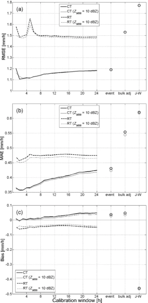
Figure 3a shows the RMSE of the rainfall rates estimated with the CT readjustment (thick solid line) for the considered durations, together with the RMSE obtained from the event adjustment, the bulk adjustment and the Joss and Waldvo-gel (J-W) relation (thick circles). The MAE and the bias of estimation are represented in Fig. 3b and c, respectively.
Figure 3 demonstrates that an improvement towards the J-W relation is achievable by assuming a uniqueZ-R rela-tionship derived from a bulk adjustment carried out on all the availableZ-R pairs. As shown in Fig. 3c, this result is due to a substantial reduction of the estimation bias. Ta-ble 1 shows the results of a comparison between the use of a linear regression on logR as in Eq. (3) and the adop-tion of the analytic expression of Eq. (2). Results in Ta-ble 1 demonstrate a general reduction of the error when
us-Fig. 3. RMSE (a), MAE (b) and bias of estimation (c) for differ-ent calibration windows and comparison with the results obtained with the event adjustment, bulk adjustment and the J-W relation. Continuous-time (CT) readjustment and real-time (RT) estimation approaches are shown, both evaluated by assuming a lower thresh-old of 0 and 10 dBZ for the reflectivity values.
ing a non-linear fit as in Eq. (2), except for the MAE with ZMIN=10 dBZ. Nevertheless, the linear regression on logR
produces a considerable bias and a substantial variability of the estimated coefficientsaˆ andbˆwith the thresholdZMIN
Table 1. Error characteristics and coefficients of the power-law relationship (Eq. 1) obtained with the adoption of a uniqueZ-Rrelation, evaluated with the linear (Eq. 3) and the non-linear (Eq. 2) methods described in Sect. 2. The corresponding results are also reported for the case of assuming a thresholdZMIN=10 dBZ.
Linear regression (Eq. 3) Non-linear regression (Eq. 2)
ZMIN=0 dBZ ZMIN=10 dBZ ZMIN=0 dBZ ZMIN=10 dBZ
ˆ
a 106 137 79 78
ˆ
b 2.02 1.64 1.81 1.82
RMSE [mm/h] 1.67 1.56 1.53 1.53
MAE [mm/h] 0.57 0.53 0.55 0.54
Bias [mm/h] –0.21 –0.16 0.05 0.04
for each rainfall event allows one to obtain a further consider-able reduction of both RMSE and MAE. This improvement is not due to a significantly lower bias but probably to the abil-ity to adapt the coefficientsaandbto account for the rainfall type (e.g., convective or stratiform precipitation), as well as event-to-event differences in radar calibration, residual clut-ter, attenuation due to wet radome and to heavy rainfall .
The “within event” CT readjustment of theZ-R relation-ship produces a further improvement of the estimation pro-cedure, which is maximum for calibration windows of 2 h, where the RMSE becomes the 28% lower than in the case of bulk adjustment. Figure 3a denotes a progressive reduc-tion of the RMSE as the width of the calibrareduc-tion window narrows. The sudden increase of the RMSE that occurs for a calibration window of one hour is due to the instability of some obtained relationships, which are evaluated on a limited number ofZ-Rpairs. On the contrary, long calibration win-dows generate more stable fits, because they are estimated on larger sets ofZ-R pairs, but as expected the correspond-ingZ-Rrelation turns out to be less accurate.
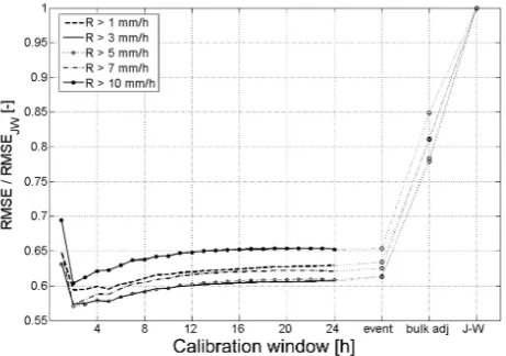
The robustness of the obtained results is confirmed in Fig. 4, which shows that the qualitative behavior of the RMSE as a function of d, as shown in Fig. 3a, is re-tained even when considering only the estimation residuals of above-threshold rainfall rates, with thresholds varying be-tween 1 and 10 mm h−1. Figure 4 shows the dimension-less ratios between the RMSE of the above threshold rainfall estimates and the corresponding (i.e., considering the same thresholds) values obtained with the J-W method. Note that the best improvements of the CT method toward the J-W method occur forZ-R pairs with thresholds between 3 and 5 mm h−1.
The whole procedure was then repeated by setting a re-flectivity threshold (ZMIN), as described in Sect. 2, and the
corresponding results are shown in Fig. 3a, b, and c with a thin solid line and thin circles. We found thatZMIN=10 dBZ
is a reasonable threshold value to adopt, which corresponds to about 0.3 mm h−1for the relation indicated above in this section, obtained from the bulk adjustment method (i.e., with
ˆ
a=79.1 and b=1.81). Such value was chosen to minimizeˆ
Fig. 4. Ratios between the RMSEs obtained by the continuous-time (CT) readjustment, event adjustment, bulk adjustment, J-W relation and the corresponding RMSEs derived by the use of the J-W relation. Results are plotted by considering rainfall rates above different thresholds between 1 and 10 mm h−1.
the resulting estimation error and therefore improving the re-moval of non-meteorological echoes. Results that stem from this method are slightly better than those obtained in the case ZMIN=0 dBZ, except for a calibration window of 2 h. This
discontinuity is due to the instability of some estimatedZ-R relationships, which in this case occurs also for calibration windows as short as 2 h. In fact, the introduction of a thresh-old onZreduces the number ofZ-Rpairs considered in each regression. On the other hand, the use of a threshold has the advantage to prevent the estimation ofZ-Rrelationships considering only very low values ofZ, which may produce large errors when used to convert high reflectivities into rain-fall rates.
3.3 Real-time (RT) estimation
Similarly to the CT procedure, the RT estimation was car-ried out for durations of the calibration window between 1 and 24 h, again for the two cases of ZMIN=0 dBZ and
The RT estimation is carried out in cross-validation mode for all the rainfall events, and the results are represented in Fig. 3a, b, and c with a thick dashed line (ZMIN=0 dBZ) and
a thin dashed line (ZMIN=10 dBZ). In this case, results are
compared to those of the J-W relation and of the bulk ad-justment. The event adjustment is not a viable method in the real-time estimation, so it will not be considered explicitly (in Fig. 3) when comparing the different approaches.
As expected, the RT method estimates turn out to be less accurate than the CT estimates, with a slight underestima-tion, on average, for all the considered durations of the cal-ibration window (see Fig. 3c). Although the estimation er-rors are, on average, lower than those of the bulk adjustment method (see Fig. 3b), the RMSE is higher for durations of the calibration window of 1, 5, and 6 h. In particular, the anoma-lous peak ford=5 h (Fig. 3a) is due to a single large error, as-sociated to a point with high reflectivity (about 39 dBZ) and no gauged rainfall on the ground, whereas theZ-R relation-ship provides a very high rainfall rate estimate (69 mm h−1). The introduction of the thresholdZMIN=10 dBZ induces
an improvement of the overall performances of the RT es-timation, in that the corresponding bias, the RMSE and the MAE are all reduced and the peaks of the RMSE are reduced as well. The comparison in Fig. 3, between the RT and CT methods, suggests that the most significant reduction of the estimation error is given by considering theZ-Rpairs at the present timeti, for calibrating the analytic relationship. This is clearly shown in the comparison of both the RMSE and MAE, between the CT and RT methods with a calibration window of one hour. In this case the procedure applied by the two methods is the same, apart from the time step con-sidered for calibrating theZ-R relationship, which isti for the CT method andti−1for the RT method.
It is worth noting that the two proposed methods allow one to obtain a considerable reduction of the mean absolute error (see Fig. 3b) if compared with the corresponding most ac-curate literature approaches that were tested in this work. In fact, the CT readjustment withd=3 h produces a MAE which is about 15% lower than for the event adjustment, while the MAE of the RT estimation withd=24 h is roughly 14% lower than in the case of using a single climatological relationship (i.e., bulk adjustment). Differently, the corresponding reduc-tion in the RMSE (Fig. 3a) is lower (6% for the CT read-justment and 4% for the RT estimation). This suggests that few largest estimation errors are retained and largely affect the RMSE, which depends on a squared measure of resid-uals. A possible explanation to this outcome is that large errors are not removed because they are not ascribable to the non-identification of a suitableZ-R relationship, but rather to other sources of error which affect the radar measurement (see Steiner et al., 1999), and particularly to observations af-fected by ground clutter contamination.
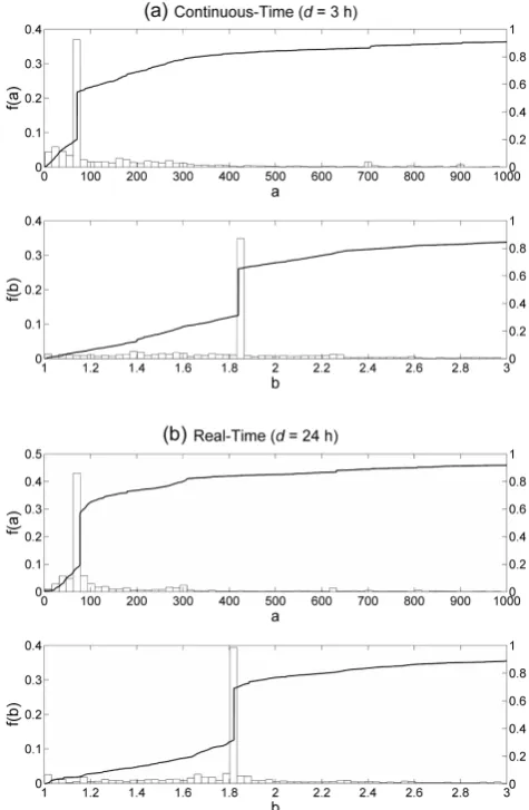
We plotted in Fig. 5 the empirical frequency distribu-tionsf (a)andf (b)of the coefficientsa andb of the esti-mated power-laws, for the two proposed methodologies. We
Fig. 5. Empirical frequency distribution (bar chart) and cumulative distribution (solid line) of the estimated coefficientsaandbof the
Z-Rpower law. Top panels (a): continuous-time (CT) readjustment (d=3 h); bottom panels (b): real-time (RT) estimation (d= 24 h).
considered a calibration window of 3 h for the CT method (Fig. 5a), and of 24 h for the RT method (Fig. 5b). The corre-sponding cumulative distributions are also represented with a continuous solid line. The spread of the estimated coef-ficients is clearly shown from the four panels of the figure. Further, one can note the sudden jump of the cumulative dis-tributions for the two coefficients assuming values a=79.1ˆ
andb=1.81. These represent the frequencies of rejected re-ˆ gressions, and amount in both cases to about 35–40% of the number of estimated values. Operationally, they are replaced with the coefficients of the bulk adjustment regression indi-cated above.
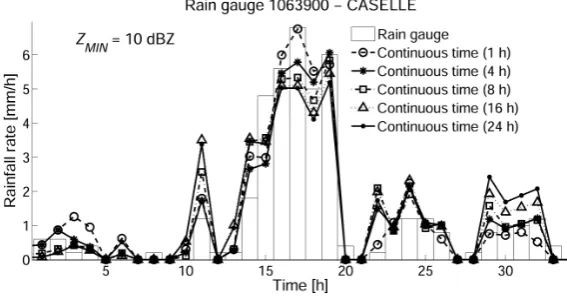
In Fig. 6 we represented a comparison between the rain-rate measured at a rain gauge during an event (white bars) and the corresponding estimates obtained with the meth-ods described in this paper, by assuming the threshold ZMIN=10 dBZ for all the cases. Again, calibration windows
Fig. 6. Comparison of rainfall rates measured at a rain gauge and the corresponding estimates for one of the rainfall events, by using the bulk adjustment method, the event adjustment, the J-W relation, the continuous-time (CT) readjustment and the real-time (RT) estimation.
Fig. 7. Comparison of rainfall rates measured at a rain gauge and the corresponding estimates for one of the rainfall events, by using the continuous-time (CT) readjustment with five different calibration windows, between 1 and 24 h.
methods. Figure 6 clearly shows the ability of the CT method to accurately estimate rainfall rates, while the J-W method al-ways provides a considerable underestimation. This picture is representative of the typical behavior of the tested method-ologies. It is shown for giving a more direct way for compar-ing the different estimation performances, while one should refer to Fig. 3 for a more objective statistical evaluation. Sim-ilarly, Fig. 7 shows a comparison between the gauged rain-fall during a selected event and the estimated values obtained by testing the CT method with five different calibration win-dows between 1 and 24 h. One can note that the five pro-cedures generally provide reliable estimates, especially for short durations of the calibration window. Indeed, even the 1-h time window provides good results. These findings are of crucial importance in that, although the CT procedure is an a posteriori analysis of rainfall rates, by waiting just 1 h from a given radar measurement, the accuracy of estimation sub-stantially improves (compared to the corresponding real-time estimates). This means that the CT method with a 1-h time window can be considered a valid “near real-time”
alterna-tive for estimation, with important implications for hydrolog-ical applications, where a 1-h lag time is a viable compromise in place of substantial quantitative improvements.
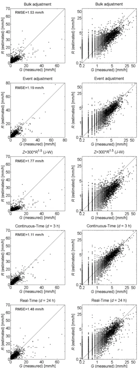
Finally, a further set of graphs is reported in Fig. 8, which shows the scatter plots between measured and estimated rain-fall rates for the five methods described in this work together with their corresponding RMSE, both in linear (left side) and logarithmic (right side) scale. Again, the selected durations of the calibration windows are 3 h for the CT method and 24 h for the RT method. Furthermore, all the scatter plots reported in Fig. 8 are obtained by setting the thresholdZMIN=10 dBZ
as explained throughout this article, in that the resulting error characteristics are slightly better than those provided by the case of thresholdZMIN=0 dBZ . One can note, in the right
Fig. 8. Scatter plots between measured and estimated rainfall rates for the five methods described in this article, both in linear (left side) and logarithmic (right side) scale. The 1:1 line is also shown in each plot. For all the five methods the thresholdZMIN=10 dBZ is adopted.
4 Conclusions
This paper presents a simple procedure for usingZ-R rela-tionships continuously updated in time, useful both for re-analysis of rainfall fields and for real time estimation, and carries out a comparison of the overall performances by test-ing different calibration windows. The outcomes of these methods are also compared with those of three other calibra-tion methods reported in the literature. The adopted proce-dure aims at producing the most accurate radar-based rainfall estimates and we do not claim any physical interpretations of the obtained relationships. The estimated coefficientsaˆandbˆ of the power-law relationships as in Eq. (1) are bounded only to prevent instability problems to occur. As a result, they are considerably spread out around those of the meanZ-R re-lation derived from the bulk adjustment method, and often assume different values from those reported in the literature. The obtained coefficientsaˆ andbˆinclude the effect of sam-pling errors of the radar measurements and the uncertainty which derives from coupling reflectivity measurements aloft with ground rainfall rates measured by the rain gauges.
Results are promising, as both the continuous-time (CT) and the real-time (RT) approaches demonstrate substantial improvements compared to the other tested methods, es-pecially when a threshold for the minimum reflectivity to consider is adopted. In particular, we suggest a calibration window of 3 h for the Z-R relationship when applying the continuous-time (CT) readjustment. In real-time (RT) esti-mation, a calibration window between roughly 8 and 24 h is a reasonable choice, which provides good accuracy of es-timation and is not affected by instability problems. Even though these results refer specifically to the case analyzed in this study, they are rather robust, since are based on more than 104estimated hourly values of precipitation.
Acknowledgements. The authors wish to thank ARPA Piemonte for providing the data and in particular S. Barbero, R. Bechini, V. Campana, R. Cremonini, D. Rabuffetti and L. Tomassone for useful discussions on this topic. The financial support of the Italian Ministry of Education and Research (grant no. 2005080287 and 2006089189) is also acknowledged.
Edited by: A. Mugnai
Reviewed by: three anonymous referees
References
Alfieri, L., Perona, P., and Burlando, P.: Optimal water allocation for an alpine hydropower system under changing scenarios, Wa-ter Resour. Manag., 20, 761–778, 2006.
Anagnostou, E. N. and Krajewski, W. F.: Real-time radar rainfall es-timation. Part I: Algorithm formulation, J. Atmos. Ocean. Tech., 16, 189–197, 1999a.
Anagnostou, E. N. and Krajewski, W. F.: Real-time radar rainfall estimation. Part II: Case study, J. Atmos. Ocean. Tech., 16, 198– 205, 1999b.
Arnaud, P., Bouvier, C., Cisneros, L., and Dominguez, R.: Influence of rainfall spatial variability on flood prediction, J. Hydrol., 260, 216–230, 2002.
Austin, P. M.: Relation between measured radar reflectivity and sur-face rainfall, Mon. Weather Rev., 115, 1053–1071, 1987. Bacchi, B. and Ranzi, R.: On the derivation of the areal reduction
factor of storms, Atmos. Res., 42, 123–135, 1996.
Battan, L. J.: Radar observations of the atmosphere, The University of Chicago Press, 1973.
Bechini, R. and Cremonini, R.: The weather radar system of north-western Italy: an advanced tool for meteorological surveillance, in: Proceedings of the Second European Conference on Radar in Meteorology and Hydrology, Delft, The Netherlands, 400–404, 18–22 November 2002.
Brandes, E. A.: Optimizing rainfall estimates with aid of radar, J. Appl. Meteorol., 14, 1339–1345, 1975.
Brath, A., Montanari, A., and Toth, E.: Analysis of the effects of different scenarios of historical data availability on the cali-bration of a spatially-distributed hydrological model, J. Hydrol., 291, 232–253, 2004.
Chiang, Y. M., Chang, F. J., Jou, B. J. D., and Lin, P. F.: Dynamic ANN for precipitation estimation and forecasting from radar ob-servations, J. Hydrol., 334, 250–261, 2007.
Chumchean, S., Seed, A., and Sharma, A.: Correcting of real-time radar rainfall bias using a Kalman filtering approach, J. Hydrol., 317, 123–137, 2006.
Ciach, G. J. and Krajewski, W. F.: Radar-rain gauge comparisons under observational uncertainties, J. Appl. Meteorol., 38, 1519– 1525, 1999.
Claps, P. and Siccardi, F.: Mediterranean Storms, BIOS, Cosenza, 1999.
Collier, C. G., Larke, P. R., and May, B. R.: A weather radar cor-rection procedure for real-time estimation of surface rainfall, Q. J. Roy. Meteor. Soc., 109, 589–608, 1983.
Cremonini, R. and Bechini, R.: Rainfall estimation in north-western Italy, using two polarimetric C-band radars and a dense real-time gauge network, 3rd GPM Workshop, ESTEC, Noordwijk, The Netherlands, 2003.
Doviak, R. J. and Zrnic, D. S.: Doppler radar and weather observa-tions, Academic Press, New York, 1984.
Gabella, M. and Amitai, E.: Radar rainfall estimates in an alpine environment using different gage adjustment techniques, Phys. Chem. Earth Pt. B, 25, 927–931, 2000.
Germann, U., Galli, G., Boscacci, M., and Bolliger, M.: Radar pre-cipitation measurement in a mountainous region, Q. J. Roy. Me-teor. Soc., 132, 1669–1692, 2006.
Joss, J. and Lee, R.: The application of radar-gauge comparisons to operational precipitation profile corrections, J. Appl. Meteorol., 34, 2612–2630, 1995.
Joss, J. and Waldvogel, A.: A method to improve the accuracy of radar-measured amounts of precipitation, in: Preprints, 14th Radar Meteorology Conf., Tucson, AZ, 237–238, 1970. Koistinen, J., Kuitunen, T., and Inkinen, M.: Area-intensity
proba-bility distributions of rainfall based on a large sample of radar data, in: Proceedings of the Fourth European Conference on Radar in Meteorology and Hydrology, Barcelona, Spain, 406– 409, 18–22 September 2006.
Lee, G. W. and Zawadzki I.: Variability of drop size distributions: time-scale dependence of the variability and its effects on rain estimation, J. Appl. Meteorol., 44, 241–255, 2005.
Legates, D. R.: Real-time calibration of radar precipitation esti-mates, Prof. Geogr., 52, 235–246, 2000.
Marshall, J. M. and Palmer W. M. K.: The distribution of raindrops with size, J. Appl. Meteorol., 5, 165–166, 1948.
Richards, W. G. and Crozier C. L.: Precipitation measurement with a C-band weather radar in Southern Ontario, Atmos. Ocean, 21, 2505–2514, 1983.
Seo, D. J. and Breidenbach, J. P.: Real-time correction of spatially nonuniform bias in radar rainfall data using rain gauge measure-ments, J. Hydrometeorol., 3, 93–111, 2002.
Smith, J. A.: Precipitation, in: Handbook of Hydrology, edited by: Maidment, D. R., McGraw-Hill, Inc, 1993.
Smith, J. A. and Krajewski, W. F.: A modeling study of rainfall rate reflectivity relationships, Water Resour. Res., 29, 2505–2514, 1993.
Steiner, M., Smith, J. A., Burges, S. J., Alonso, C. V., and Dar-den, R. W.: Effect of bias adjustment and rain gauge data qual-ity control on radar rainfall estimation, Water Resour. Res., 35, 2487–2503, 1999.
Ulbrich, C. W. and Lee, L. G.: Rainfall measurement error by WSR-88D radars due to variations inZ-Rlaw parameters and the radar constant, J. Atmos. Ocean. Tech., 16, 1017–1024, 1999. Woodley, W. L., Olsen, A. R., Herndon, A., and Wiggert, V.:
Com-parison of gauge and radar methods of convective rain measure-ment, J. Appl. Meteorol., 14, 909–928, 1975.