Intervertebral Disc Structure and Mechanical Function Under Physiological Loading Quantified Non-invasively Utilizing MRI and Image Registration

(1)

University of Pennsylvania

ScholarlyCommons

Publicly Accessible Penn Dissertations

1-1-2014

Intervertebral Disc Structure and Mechanical

Function Under Physiological Loading Quantified

Non-invasively Utilizing MRI and Image

Registration

Jonathon H. Yoder

University of Pennsylvania, [email protected]

Follow this and additional works at:http://repository.upenn.edu/edissertations

Part of theBiomechanics Commons,Biomedical Commons, and theRadiology Commons

This paper is posted at ScholarlyCommons.http://repository.upenn.edu/edissertations/1511

For more information, please [email protected].

Recommended Citation

Yoder, Jonathon H., "Intervertebral Disc Structure and Mechanical Function Under Physiological Loading Quantified Non-invasively Utilizing MRI and Image Registration" (2014).Publicly Accessible Penn Dissertations. 1511.

(2)

Intervertebral Disc Structure and Mechanical Function Under

Physiological Loading Quantified Non-invasively Utilizing MRI and

Image Registration

Abstract

The intervertebral discs (IVD) functions to permit motion, distribute load, and dissipate energy in the spine. It performs these functions through its heterogeneous structural organization and biochemical composition consisting of several tissue substructures: the central gelatinous nucleus pulposus (NP), the surrounding fiber reinforced layered annulus fibrosus (AF), and the cartilaginous endplates (CEP) that are positioned between the NP and vertebral endplates. Each tissue contributes individually to overall disc mechanics and by interacting with adjacent tissues. Disruption of the disc's tissues through aging, degeneration, or tear will not only alter the affected tissue mechanical properties, but also the mechanical behavior of adjacent tissues and, ultimately, overall disc segment function. Thus, there is a need to measure disc tissue and segment mechanics in the intact disc so that interactions between substructures are not disrupted. Such measurements would be valuable to study mechanisms of disc function and degeneration, and develop and evaluate surgical

procedures and therapeutic implants. The objectives of this study were to develop, validate, and apply methods to visualize and quantify IVD substructure geometry and track internal deformations for intact human discs under axial compression. The CEP and AF were visualized through MRI parameter mapping and image sequence optimization for ideal contrast. High-resolution images enabled geometric measurements. Axial compression was performed using a custom-built loading device that permitted long relaxation times outside of the MRI, 300 m isotropic resolution images were acquired, and image registration methods applied to measure 3D internal strain. In conclusion, new methods to visualize and quantify CEP thickness, annular tear detection and geometric quantification, and non-invasively measure 3D internal disc strains were established. No correlation was found between CEP thickness and disc level; however the periphery was significantly thicker compared to central locations. Clear distinction of adjacent AF lamellae enabled annular tear detection and detailed geometric quantification. Annular tears demonstrated "non-classic" geometry through interconnecting radial, circumferential, and perinuclear formations. Regional strain inhomogeneity was observed qualitatively and quantitatively. Variation in strain magnitudes might be explained by geometry in axial and circumferential strain while peak radial strain in the posterior AF may have important implications for disc herniation.

Degree Type

Dissertation

Degree Name

Doctor of Philosophy (PhD)

Graduate Group

Mechanical Engineering & Applied Mechanics

First Advisor

Dawn M. Elliott

(3)

Keywords

annulus fibrosus, axial compression, image registration, internal strain, intervertebral disc, magnetic resonance imaging

Subject Categories

Biomechanics | Biomedical | Radiology

(4)

INTERVERTEBRAL DISC STRUCTURE AND MECHANICAL

FUNCTION UNDER PHYSIOLOGICAL LOADING QUANTIFIED

NON-INVASIVELY UTILIZING MRI AND IMAGE

REGISTRATION

Jonathon Henry Yoder

A DISSERTATION

in

Mechanical Engineering and Applied Mechanics

Presented to the Faculties of the University of Pennsylvania

in

Partial Fulfillment of the Requirements for the

Degree of Doctor of Philosophy

2014

Supervisor of Dissertation

____________________

Dawn M. Elliott, Professor – Director of Biomedical Engineering University of Delaware

Graduate Group Chairperson

____________________

Prashant Purohit, Chair and Associate Professor MEAM

Dissertation Committee:

Louis J Soslowsky, Fairhill Professor Orthopaedic Surgery and Professor Bioengineering James C Gee, Associate Professor Radiologic Science in Radiology

Prashant Purohit, Chair and Associate Professor MEAM Beth A Winkelstein, Professor Bioengineering

(5)

ii

ABSTRACT

INTERVERTEBRAL DISC STRUCTURE AND MECHANICAL FUNCTION UNDER

PHYSIOLOGICAL LOADING QUANTIFIED NON-INVASIVELY UTILIZING MRI

AND IMAGE REGISTRATION

Jonathon H Yoder

Dawn M Elliott

The intervertebral discs (IVD) functions to permit motion, distribute load, and dissipate

energy in the spine. It performs these functions through its heterogeneous structural

organization and biochemical composition consisting of several tissue substructures: the

central gelatinous nucleus pulposus (NP), the surrounding fiber reinforced layered

annulus fibrosus (AF), and the cartilaginous endplates (CEP) that are positioned between

the NP and vertebral endplates. Each tissue contributes individually to overall disc

mechanics and by interacting with adjacent tissues. Disruption of the disc’s tissues

through aging, degeneration, or tear will not only alter the affected tissue mechanical

properties, but also the mechanical behavior of adjacent tissues and, ultimately, overall

disc segment function. Thus, there is a need to measure disc tissue and segment

mechanics in the intact disc so that interactions between substructures are not disrupted.

Such measurements would be valuable to study mechanisms of disc function and

degeneration, and develop and evaluate surgical procedures and therapeutic implants. The

(6)

iii

quantify IVD substructure geometry and track internal deformations for intact human

discs under axial compression. The CEP and AF were visualized through MRI parameter

mapping and image sequence optimization for ideal contrast. High-resolution images

enabled geometric measurements. Axial compression was performed using a custom-built

loading device that permitted long relaxation times outside of the MRI, 300 m isotropic

resolution images were acquired, and image registration methods applied to measure 3D

internal strain. In conclusion, new methods to visualize and quantify CEP thickness,

annular tear detection and geometric quantification, and non-invasively measure 3D

internal disc strains were established. No correlation was found between CEP thickness

and disc level; however the periphery was significantly thicker compared to central

locations. Clear distinction of adjacent AF lamellae enabled annular tear detection and

detailed geometric quantification. Annular tears demonstrated “non-classic” geometry

through interconnecting radial, circumferential, and perinuclear formations. Regional

strain inhomogeneity was observed qualitatively and quantitatively. Variation in strain

magnitudes might be explained by geometry in axial and circumferential strain while

peak radial strain in the posterior AF may have important implications for disc herniation.

(7)

iv

List of Tables

Table 1: Average (±standard deviation) T1 values for a healthy and degenerate disc substructures. ... 27 Table 2: Average T1 and T2 values for a healthy and degenerate disc substructures. ... 43 Table 3: Tear severity measurements. Type: R = radial, C = circumferential, PN =

perinuclear. Location: L = lateral, TL = trans-lateral, A = anterior, AL = antero-lateral, PL = postero-lateral... 45 Table 4: Matrix of ANTs registration parameters (transformation models, similarity

metrics, regularization techniques). MI = mutual information, MSQ = mean squared difference, CC = fast cross correlation, PR = cross correlation, PSE = point set expectation, DMFFD = directly manipulated free form deformation. Adapted from Avants et al. 2011 ... 64 Table 5: Parametric analysis variable matrix used for registrations ... 65 Table 1: Mean ± standard deviation of stress and strain for each applied loading

condition. Note that Applied Compression represents grip-to-grip applied strains that are compressive and that these compressive boundary conditions induce

negative axial strain. AF = annulus fibrosus, Ezz = axial strain, E= circumferential

strain, Err = radial strain. Stress calculated as load divided by area from axial

reference MR image. Strains averaged over entire AF volume for each disc. N= 9. 91 Table 7: Global annulus fibrosus strain values (average ± standard deviation). ... 111 Table 8: Results for regional axial (Ezz) strain values (mean ± standard deviation) under

5%, 10%, and 15% axial compression. Region definitions: axial disc height (M = middle region, S/I = attachment region), radial position (O = outer annulus, I = inner annulus), and circumferential position (A = anterior, A-L = anterior-lateral, L = lateral, P-L = posterior-lateral, P = posterior). Three comparisons were made along each axis to assess regional variance: 1. Axial column analyzed superior/interior vs. middle region disc height within the outer and inner annulus for each circumferential position (A, A-L, L, P-L, P). Circumferential column analyzed the differences between (A, A-L, L, P-L, P) within the outer and inner annulus for each axial disc-height position, and 3. Radial column analyzed inner vs. outer annulus within (A, A-L, A-L, P-A-L, P) for each axial disc-height position. Significance (* = p < 0.05) and trend (ŧ = 0.05 < p < 0.10) ... 125 Table 9: Results for regional circumferential (Eϕϕ) strain values (mean ± standard

deviation) under 5%, 10%, and 15% axial compression. Region definitions: axial disc height (M = middle region, S/I = attachment region), radial position (O = outer annulus, I = inner annulus), and circumferential position (A = anterior, A-L = anterior-lateral, L = lateral, P-L = posterior-lateral, P = posterior). Three

comparisons were made along each axis to assess regional variance: 1. Axial column analyzed superior/interior vs. middle region disc height within the outer and inner annulus for each circumferential position (A, A-L, L, P-L, P). Circumferential column analyzed the differences between (A, A-L, L, P-L, P) within the outer and inner annulus for each axial disc-height position, and 3. Radial column analyzed inner vs. outer annulus within (A, A-L, L, P-L, P) for each axial disc-height position. Significance (* = p < 0.05) and trend (ŧ = 0.05 < p < 0.10) ... 126 Table 10: Results for regional radial (Err) strain values (mean ± standard deviation) under

(10)

vii

middle region, S/I = attachment region), radial position (O = outer annulus, I = inner annulus), and circumferential position (A = anterior, A-L = anterior-lateral, L = lateral, P-L = posterior-lateral, P = posterior). Three comparisons were made along each axis to assess regional variance: 1. Axial column analyzed superior/interior vs. middle region disc height within the outer and inner annulus for each circumferential position (A, A-L, L, P-L, P). Circumferential column analyzed the differences between (A, A-L, L, P-L, P) within the outer and inner annulus for each axial disc-height position, and 3. Radial column analyzed inner vs. outer annulus within (A, A-L, A-L, P-A-L, P) for each axial disc-height position. Significance (* = p < 0.05) and trend (ŧ = 0.05 < p < 0.10). ... 127 Table 11: Results for regional radial (Eϕr) strain values (mean ± standard deviation) under

(11)

viii

List of Illustrations

Figure 1: Representative lumbar spine image and the intervertebral disc sub-structures. .. 6 Figure 2: Magnetic resonance images illustrating different stages of human lumbar

degeneration. (A) A healthy disc exhibiting distinct AF lamellae and central NP region. (B) A disc exhibiting early stages of degeneration, including moderate height reduction, decreased NP signal intensity and inward bulging of AF lamellae (*). (C) A disc exhibiting advanced stages of degeneration, including severely reduced height, large fissures (*) and generalized structural deterioration.(Smith, Nerurkar et al. 2011) ... 10 Figure 3: Representative annular and intervertebral disc defects. (Vernon-Roberts, Moore et al. 2007) ... 11 Figure 4: Pfirmann grading scale displaying degenerative changes visualized in MR

(Pfirrmann, Metzdorf et al. 2001). ... 13 Figure 5: T2 correlations to T1ρ and Pfirrmann from Elliot Lab lumbar spine database

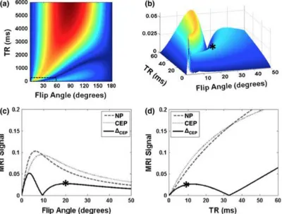
collected over several years for a multitude of studies ... 13 Figure 6: Graphical overview of image registration ... 19 Figure 7: Representative T1 parameter maps at 7T: (A) T1 healthy, (B) T1 degenerate . 23 Figure 8: Computed MRI signals and image contrast at 7T: (a) NP-CEP image contrast

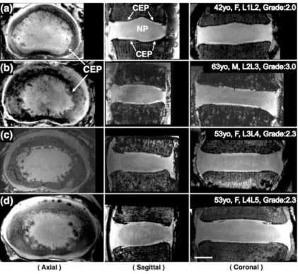
(ΔCEP) according to Equation 3, over the full range of the parameters flip angle and TR. (b) Close-up 3D view within the small dashed box in (a). Asterisk (*) indicates the point chosen as optimal. (c,d) Computed NP (dashed) and CEP (dotted) MRI signals, and image contrast (ΔCEP, solid) versus flip angle at optimal TR (9 ms) (c) and versus TR at optimal flip angle (20°) (d). ... 28 Figure 9: MRI images of four different specimens with 200 μm isotropic resolution

acquired at 7T. Three-plane views reformatted from the same isotropic dataset of each specimen clearly demonstrate the CEP’s (arrows) clearly, which are located between the vertebral body and the NP. Axial views show that the shape and size of the CEP can vary considerably for different subjects and levels: (a) 47 years, female, L1L2; (b) 63 years, male, L2L3; (c) 53 years, female, L3L4; (d) 53 years, female, L4L5. Scale bar = 1 cm ... 29 Figure 10: MRI and histology images of the same specimen (63 years, male, L2L3, Grade

2.6). Axial (a) and coronal (b) FLASH MRI of the whole disc, showing approximate locations of biopsy punches used for histological analysis. (c) Representative

histology section of the CEP stained with Alcian blue (glycosaminoglycans) and picrosirius red (collagen) showing adjacent NP and vertebral bone. (d) Von Kossa staining of an undecalcified section, showing regions of bone distinct from CEP and minimal CEP calcification. (Scale bars in (a) and (b) = 1 cm and in (c) and (d) = 0.5 mm) ... 30 Figure 11: CEP thickness in specimens, as measured on mid-sagittal MRI slices: (a) at

different disc levels (b) at different anterior-posterior locations (C-center, A5, A10 = 5 and 10mm off the center towards anterior, P5, P10 = 5 and 10 mm off the center towards posterior). Letters on top of error bars indicate significance (p<0.005) between measured locations. ... 31 Figure 12: Representative parameter maps at 7T: (A) T1 healthy, (B) T1 degenerate, (C)

(12)

ix

Figure 13: Computed AF MRI signals and image contrast at 7T. (a) Normalized AF signal intensity according to Equation 6 over the full range of parameters TR and TE. (b) AF image contrast based on Equation 7 utilizing the maximum and

minimum AF signal intensities. (c,d) Computed AF max (dashed), AF min (dotted) MRI signals, and image contrast (solid) at optimal TE (34 ms) (c) and versus TE at optimal TR (3000 ms) (d). ... 44 Figure 14: Representative images for (A) Radial, (B) Perinuclear, and (C)

Circumferential tears. Left column shows raw TSE images and right shows 3D fusion volume rendering for each tear, respectively ... 46 Figure 15: Volume renderings of tears: (A-B) Radial and (C) Perinuclear/Radial –

coronal views; (D-E) Circumferential – axial and coronal views of the same

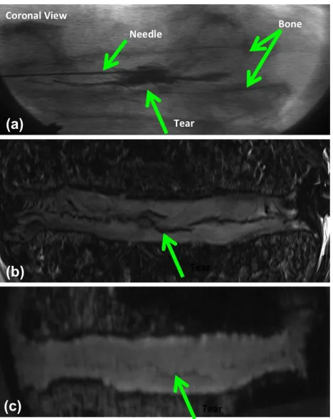
specimen. ... 47 Figure 16: Three matched images of a radial tear with different imaging: (a) fluoroscopic

coronal view with radiographic dye, (b) T2 weighted TSE, and (c) T1 weighted FLASH ... 47 Figure 17: MRI loading frame integration with Instron 8874 ... 51 Figure 18: Effect of signal to noise ratio (SNR) on disc positioning within the MRI. Red

arrow indicates the direction of lost signal within the RF coil. Clinically relevant anatomic orientation (Left Side) results in decreased posterior AF lamellar

distinction (Orange Arrow). Lateral positioning of the disc (Right Side) enables the spine axis and B0 (Blue Circle: dot indicates spine axis and B0 direction) to be parallel, decreasing banding artifacts within the disc during image acquisition. ... 53 Figure 19: Integration of loading device with MRI and RF coil: (1) Placement of the

transmit piece of the coil in the direction of B0 on the MRI patient table, (2) loading frame slides over the transmit piece, and the (3) receive array slides directly over the disc’s location. ... 54 Figure 20: Representative mid-axial MR images with (A) and without (B) loading frame. Signal to noise ratio (SNR) was measured using a region selected within the agarose (Green) to represent signal, as these samples come from different lumbar levels (Noise – White). ... 55 Figure 21: Representative image depicting area and length measurements in the Coronal

and Sagittal plane to determine an average disc-height across the entire disc volume. ... 57 Figure 22: Representative (A) reference and (B) deformed labeled images. Labels cover

the SVB, IVB, AF lamellae, and defects. Arrows indicate differences between reference and deformed images. ... 62 Figure 23: Overlay of reference and reconstructed labels. Arrows indicate regions where

individual pixels are not aligned. ... 62 Figure 24: Reconstructed image displaying the effect of Gaussian (A) vs. B-spline (B)

regularization technique. Note the unnatural swirling pattern within the NP and vertebrae in the Gaussian regularization. ... 65 Figure 25: Segmentation of AAF (red) and PAF (blue) using ITK-SNAP. Each region

was defined based on visible lamellae within each IVD. ... 67 Figure 26: Representative plot on the effect of B-splines on AAF and PAF (A) Avg (B)

(13)

x

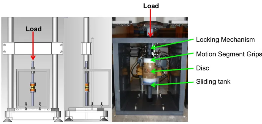
Figure 27: Representative (A) radial and (B) axial strain maps generated in ANTs. (C) Radial strains and (D) Axial strains measured in the AAF, PAF, and IVD in ANTs (intact white, nucleotomy checkered) and Vic2D (intact black, nucleotomy striped), == p ≤ 0.05 & — p ≤ 0.10... 70 Figure 1: (A) Loading frame interfaced with Instron (red arrow), showing locking

mechanism, segment grips, disc, and sliding tank (white arrows). (B) Loading frame integrated with RF coil (green arrows) in MRI. B0 = direction of magnetic field. .. 77 Figure 2: Images (A – C) are oriented to show coronal (left), axial (top-right), and sagittal

(bottom) planes. (A) Representative MRI data set. (B) The volume used for strain analysis (pink). (C) Annulus fibrosus regions of interest defined in the mid-axial plane: A=anterior (red), A-L=anterior-lateral (green), L=lateral (purple), P-L= posterior-lateral (yellow), P=posterior (aqua)... 79 Figure 3: Pictorial representation of the image registration process, resultant warp field,

and displacement map. The reference image is registered to the deformed image defining a warp field that prescribes how structures within the reference image are mapped to the deformed image. The deformation gradient tensor is applied to calculate the Lagrnagian strain tensor... 80 Figure 4: (A) Generation of lamellar structure labels using Sobel edge detection (red),

shown in three planes. A representative label is shown in green. (B-C) Five identified lamellar labels, shown in mid-axial view and as 3D projections,

respectively. Labels identified by white arrow. ... 82 Figure 5: Transformation of Cartesian coordinates to local disc coordinates using the

disc’s outer contour, scaled to intersect each voxel: (A) circumferential basis vectors defined by the contour’s tangent; (B) radial basis vectors defined by the contour’s normal. Note the complex vector directions imposed by the lamellar curvature. .... 85 Figure 6: Registration of a representative lamellar label (green), shown in coronal (left),

axial (top-right), and sagittal (bottom) views. Difference between original and registered label is small (red), demonstrating good registration. Scale bar = 1cm ... 88 Figure 7: Axial strains for all discs obtained by manual measurement and by image

registration, showing good agreement (r2=0.79, p<0.05). ... 89 Figure 8: Strain maps for 10% axial compression in a representative disc: (A) axial strain in coronal and sagittal views (left and right, respectively); (B) circumferential strain in axial view; (C) radial strain in axial view. Scale bar = 5 cm. ... 90 Figure 9: Mean (standard deviation) of AF regional strain at mid-disc height when loaded

to 15% compression for (A) axial, (B) circumferential, and (C) radial strain.

A=Anterior, A-L=Anterior-Lateral, L=Lateral, P=L=Posterior-Lateral, P=Posterior. Region locations are shown in Figure 2C. A solid line represents significance

p<0.05 and dashed line a trend 0.05<p<0.10. ... 91 Figure 35: Representative segmentation process for defining disc regions: (A) Automatic

NP (blue), inner AF (green), and outer AF (red), (B) Axial height division into superior, middle, and inferior disc regions, and (C) Subdivision into anterior: A, anterior-lateral: A-L, lateral: L, posterior-lateral: P-L, and posteriorL: P annulus within each axial height division. White scale bar = 1 cm. ... 107 Figure 36: Representative middle third disc height anterior outer annulus axial strain

(14)

xi

distribution. Mean strain values (solid black line) were reported for each region. One standard deviation (dashed black line) is shown for reference. ... 107 Figure 37: Reported regional (average ± standard deviation) mean strain values for

inferior (red) and superior (green) annulus fibrosus at 5%, 10%, and 15% axial compression for [A] – axial (Ezz), [B] – circumferential (E), [C] – radial (Err), and [D] – in-plane shear (Er). ... 110 Figure 38: Regional strain bar charts (mean ± standard deviation) comparing the inner

(left-hand side) and outer (right-hand side) attachment region (solid) vs. middle (dotted) AF regions under 15% axial compression for axial [A / B], circumferential [C / D], radial [E / F], and in-plane shear [G / H] at 15% axial compression.

Regions: anterior (A – red), anterior-lateral (A-L – green), lateral (L – blue),

posterior-lateral (P-L – orange), and posterior (P – turquoise) annulus. Significance: solid line p ≤ 0.05. Trend: dashed line 0.05 ≤ p ≤ 0.10. ... 113 Figure 39: Regional strain bar charts (mean ± standard deviation) comparing the

circumferential positions (A, A-L, L, P-L, and P) along the middle [left-hand side] and attachment region [right-hand side] disc height within the outer (solid) and inner (dashed) AF regions under 15% axial compression for axial [A / B], circumferential [C / D], radial [E / F], and in-plane shear [G / H] at 15% axial compression.

Regions: anterior (A – red), anterior-lateral (A-L – green), lateral (L – blue),

posterior-lateral (P-L – orange), and posterior (P – turquoise) annulus. Significance: solid line p ≤ 0.05. Trend: dashed line 0.05 ≤ p ≤ 0.10. ... 116 Figure 40: Regional strain bar charts (mean ± standard deviation) comparing the middle

[left-hand side] and attachment region [right-hand side] disc height outer (solid) and inner (dashed) AF regions under 15% axial compression for axial [A / B],

circumferential [C / D], radial [E / F], and in-plane shear [G / H] at 15% axial compression. Regions: anterior (A – red), anterior-lateral (A-L – green), lateral (L – blue), posterior-lateral (P-L – orange), and posterior (P – turquoise) annulus.

Significance: solid line p ≤ 0.05. Trend: dashed line 0.05 ≤ p ≤ 0.10. ... 118 Figure 41: Proof of concept balloon loading placement: (A) Unpressurized placement in

center of NP under fluoroscopic guidance, (B) Pressurized balloon, and (C) Securing of balloon. ... 135 Figure 42: Proof of concept balloon visualization comparing an intact bovine motion

(15)

1

CHAPTER 1 Introduction

The intervertebral disc (IVD) functions to permit motion of the spine while

distributing the multidirectional loads experienced during daily activities, including

tension, compression, torsion, and bending. Intervertebral disc degeneration widely

afflicts the aging population, often manifesting itself in low back pain. This progressive

and irreversible process causes deleterious changes to the disc’s structural integrity,

mechanical function, and nutritional pathways. The current surgical standard of care for

painful disc degeneration is limited to disc removal, followed by superior and inferior

vertebral body fusion or total disc replacement. Fusion results in a loss of motion and the

ability to distribute load. Total disc replacement attempts to preserve mobility, but does

not replicate the native disc load distribution characteristics. Quantification of internal

IVD mechanics can improve knowledge of the effect of degeneration on disc mechanical

function. This knowledge will provide crucial design criteria to better recapitulate healthy

disc structure and function, and thus improve treatment options.

Measuring disc internal mechanics is a complicated challenge; in situ boundary

condition replication is difficult with excised tissue testing samples. Motion segment

testing permits the study of overall disc stress and strain behavior, but it does not present

detail of the discs internal mechanics and interactions between its constituents. Prior

experimental studies have attempted to study the IVD internal deformations; however

they are limited to physical marker insertion or entire disc bisection, disrupting the discs

structural integrity. Physical markers may move separately from the surrounding tissue

and bisection depressurizes the NP, altering the AF mechanics. Magnetic resonance

(16)

2

non-invasive technique to visualize the disc’s substructures in two-dimensions (2D). This

technique has only been applied to measure 2D strain under single loads. However, the

IVD deforms in three-dimensions (3D). Single 2D images are not able to capture

out-of-plane deformations, which are typical of a loaded disc. Work within this dissertation will

develop techniques utilizing 3D MRI and image registration to allow intervertebral disc

structural visualization and the quantification of its deformations under load. The overall

objective of this dissertation is to measure the disc’s 3D internal deformations when

subjected to physiological loading, and more specifically, the effect of incremental axial

deformations on the regional annulus fibrosus (AF) mechanics.

Chapter 2 will provide background on the IVD and explain the structure,

composition, and mechanical function of healthy discs as well as the effects of

degeneration. Additionally, a thorough review of internal deformations within the IVD,

medical image analysis, and an introduction to Advanced Normalization Tools for image

registration will be presented.

Current MRI techniques for visualizing the detailed IVD structure have been

limited to single 2D images in one of the primary orthogonal planes: sagittal, coronal, or

transverse. Chapter 3 will develop a 3D MRI sequence to visualize and distinguish the

cartilaginous endplate (CEP). As the IVD degenerates, there is a loss of structural

integrity causing the CEP to become sclerotic. The imaging techniques developed in

Chapter 3 will then be applied to detecting and quantifying CEP thickness.

Chapter 4 will further visualize and distinguish the annulus fibrosus lamellae

within the IVD. A 3D MRI sequence will enable the ability to differentiate between

(17)

3

circumferential, perinuclear), rim lesions, and Schmorl’s nodes. The high-resolution 3D

images will then be applied to the clinically relevant problem to non-invasively

characterize and quantify annular deformities which are linked to low back pain and alter

disc mechanics. The ability to visualize AF lamellae in 3D will be applied to track

internal deformations within the disc under physiological loading in Chapters 7-8.

Chapter 5 describes an MRI compatible loading device designed to apply

incremental amounts of axial compression, maintain disc hydration, and integrate with a

curved RF coil. The developed loading frame will enable disc image acquisition in both a

reference and deformed state with the optimized sequence from Chapter 4.

Image registration is considered a promising soft tissue (e.g., pulmonary and

cardiovascular tissues, and ligament) strain analysis technique utilizing medical images.

Chapter 6 will establish the use of Advanced Normalization Tools (ANTs), an image

registration software for disc registration and optimize its parameters for 2D strain

analysis. The use of manual segmentation tools will enable registration accuracy

verification and strain measurements across user-defined regions. Registration strain

measurements before and after nucleotomy will be compared with previously published

texture correlation methods. Image registration optimization in 2D will be translated to

3D in chapters 7-8.

In Chapter 7, the high-resolution isotropic MR imaging sequence (Chapter 4),

MRI safe loading frame (Chapter 5), and optimized image registration parameters

(Chapter 6) will enable 3D internal deformation measurements in intact human discs.

Intervertebral disc substructures work together and distribute multi-directional loading in

(18)

4

strain distributions under physiological loading is limited. Experimental whole-disc

testing is limited to providing global disc load and deformation details, not yielding

internal mechanics information. The effect of incremental amounts of axial compression

on the regional strain variance will be reported along the mid-axial disc height.

Chapter 8 will expand upon the techniques developed in Chapters 3 – 6 to assess

the internal regional strain properties of the IVD. Regional strain analysis has been

limited to mid-axial, ex-vivo tissue testing, surface strain measurements, and

two-dimensional internal analysis. A complete 3D internal strain analysis will be performed

segmenting the disc into radial (i.e., inner and outer), circumferential (i.e., anterior,

lateral, and posterior) and axial (i.e., inferior, medial, and superior) components.

The developed capabilities to measure 3D internal strain within the disc, the

results from this dissertation, and proposed future studies involving the assessment of

degeneration, different loading schemes, and clinical treatments will be discussed in

(19)

5

CHAPTER 2 Background

2.1. Clinical Significance

Intervertebral disc (IVD) degeneration is a progressive disease strongly linked to

low back pain (Frymoyer 1988, Andersson 1999, Adams 2004, Adams and Dolan 2005).

This ailment debilitates more than 5 million Americans and is the second most frequent

reason for physician visits (Deyo and Tsui-Wu 1987, Luo, Pietrobon et al. 2004). Its

estimated $100 billion societal cost in the United States (Katz 2006) mandates increased

knowledge of the effects of this disease. Current surgical treatment options for painful

disc degeneration is limited to disc removal, followed by either superior and inferior

vertebral body fusion or total disc replacement (Schizas, Kulik et al.). Fusion results in a

loss of motion and load distribution. Total disc replacement attempts to preserve mobility

but does not replicate the native disc load distribution characteristics (Costi, Freeman et

al.). Degeneration greatly affects the IVD and its constituents; it is associated with

mechanical damage, biological degradation, and a loss of nutritional pathways (Martin,

Boxell et al. 2002). Studies have shown that individuals, who undergo recurring

compressive and torsional motion, have a higher incidence of disc degeneration

compared to the general population (Kumar 2004, Hangai, Kaneoka et al. 2009). The

factors that cause disease progression, including interactions of mechanical,

compositional, structural, and cellular changes, are not well understood (Buckwalter and

Mow 2000). The primary function of the disc is mechanical; however the understanding

of disc internal deformations is limited to 2D work (O'Connell, Malhotra et al. ,

(20)

6

motivates the current study to examine the disc’s 3D internal mechanics, quantify the

effects of degeneration, and explore potential restorative techniques for AF mechanics.

2.2. Intervertebral Disc Structure

The spine is a column-like structure that is made up of alternating vertebral bodies

(VB) that encapsulate the intervertebral discs (IVD) acellular soft-tissues. The IVD

sub-structures (Figure 1) comprise of the nucleus pulposus (NP), annulus fibrosus (AF), and

the cartilaginous endplates (CEP).

Figure 1: Representative lumbar spine image and the intervertebral disc sub-structures.

The NP is a hydrated, gel-like structure made up of water, proteoglycan, and type

II-collagen that primarily aids the IVD during compression (Pearce, Grimmer et al.

1987). The NP is circumferentially encapsulated by the AF, which is made up of highly

organized concentric lamellae. Each layer of lamellae has alternating fiber orientations

28°-43° above and below the transverse plane (Marchand and Ahmed 1990); with the

angle increasing from outer to inner AF. These fibers are made up of collagen bundles

that are embedded in a matrix of proteoglycans and non-fibrillar collagens. Along the

(21)

7

in type I collagen (Buckwalter 1995); resulting in less distinctive lamellae. Lamellae

thickness varies by location (anterior/posterior/lateral) within the disc and becomes

thicker towards the NP ranging from 140 – 520 μm (Marchand and Ahmed 1990). The

AF outer lamella fibers are attached to the vertebra, while the inner lamellas merge with

the CEP. The CEP is a very thin layer of hyaline-like cartilage, ranging from 450 – 800

μm positioned between the vertebral endplates and the NP (Roberts, Menage et al. 1989,

Marchand and Ahmed 1990, Roberts, Menage et al. 1993, Moore 2000, Urban and

Roberts 2003). It provides a mechanical barrier between the pressurized NP and the VB,

acting as a gateway for nutrient transport from blood vessels into the disc (Roberts,

Menage et al. 1993, Moore 2000, Urban and Roberts 2003). The structure and

composition of the disc is strongly linked to its mechanical function (Buckwalter and

Mow 2000).

2.3. Disc Mechanical Function

The intervertebral discs sub-structures (nucleus pulposus – NP, annulus fibrosus –

AF, and cartilaginous endplate – CEP) function to distribute multi-directional loads,

which are applied to the disc during daily activities that relate to tension, compression,

torsion, and bending with stresses ranging from 0.1-2.3 MPa (Nachemson and Morris

1963, Wilke, Neef et al. 1999). The disc acts as a pressurized vessel, under load the NP

exhibits viscoelastic properties (Iatridis, Weidenbaum et al. 1996, Iatridis, Setton et al.

1997), where the pressurization of the NP transfers hoop stresses radially to the

anisotropic nonlinear AF. The alternating AF collagen fiber network permits resistance to

(22)

8

circumferential stress from the NP bulging under physiological loading. The proposed

work will focus on the internal strains seen during physiological compressive loads.

Motion-segment (bone-disc-bone) testing has been extensively performed in

compression analyzing both the static (Stokes, Laible et al. , Koeller, Funke et al. 1984,

Keller, Spengler et al. 1987, Cannella, Arthur et al. 2008) and dynamic (Adams and

Hutton 1983, Liu, Njus et al. 1983, Hansson, Keller et al. 1987, Race, Broom et al. 2000,

Riches, Dhillon et al. 2002, Johannessen, Vresilovic et al. 2004, van der Veen, van Dieen

et al. 2007, Korecki, MacLean et al. 2008, Wang, Wu et al. 2008) responses of the disc.

Disc height decreases under axial compression, resulting in an intradiscal pressure

increase. The reported disc’s compressive stiffness and modulus are 1.73 kN/mm and

3-10MPa (Nachemson, Schultz et al. 1979, Shea, Takeuchi et al. 1994, Beckstein, Sen et al.

2008) respectively. Under extended creep loading the NP transfers load to the annulus.

The thin posterior annulus sustains high strains (Stokes 1987, Heuer, Schmidt et al. 2008)

resulting in stress concentrations (Adams, McMillan et al. 1996, Edwards, Ordway et al.

2001). Radiographic measures have shown the endplate to bulge under increasing

amounts of load (Holmes, Hukins et al. 1993).

Torsional shear modulus ranges between 2-9 MPa (Abumi, Panjabi et al. 1990,

Elliott and Sarver 2004, Beckstein, Espinoza Orias et al. 2007) within the AF, where the

disc experiences 1-2° of torsion in-vivo (Adams and Hutton 1981). Both the facet joints

and annulus resist torsion (Shirazi-Adl 1994, Krismer, Haid et al. 1996) with the annulus

bearing upwards of 77% (Yingling and McGill 1999). Surface strain measurements have

shown the posterior lateral region to experience the greatest strain under torsion (Stokes

(23)

9

linked to degeneration by the derangement of the AF lamellae at low magnitudes (Farfan

1969, Farfan, Cossette et al. 1970) and to increased risk of herniation under combined

loading conditions (Drake, Aultman et al. 2005).

2.4. Disc Degeneration

Degeneration of the IVD causes progressive changes to the disc’s structural

integrity (Figure 2), mechanical function, and loss of nutritional pathways; the

interactions of these changes are not well understood. During IVD degeneration the

proteoglycans breakdown, resulting in a pressure loss and the ability to maintain

hydration within the NP. This pressure and hydration loss subsequently causes a

decrease in compressive stiffness (Buckwalter 1995, Nguyen, Johannessen et al.

2008). These changes in biochemical composition as a result of degeneration lead to

a loss in fixed charge density (Urban and McMullin 1985, Urban and McMullin

1988). Consequently, the AF bears most of the loads within the IVD (Tsantrizos, Ito

et al. 2005), leading to inward bulging of the AF (Brinckmann and Grootenboer

1991), disorganization, and thickening. Thickening increases collagen cross-linking

(Pokharna and Phillips 1998), which can lead to annular tears (Thompson, Pearce et

al. 1990, Adams 2004) and ultimately disc herniation. The inner AF undergoes an

increase in collagen content with type II collagen fibrils becoming type I.

(Weidenbaum and Iatridis 2006). This change in fibril type makes the distinction

between NP and AF less apparent. Additionally, the CEP becomes sclerotic and loses

vascular contact, which in turn causes decreased permeability, nutritional loss, and

(24)

10

Roberts, Urban et al. 1996, Grignon, Grignon et al. 2000, Bibby, Jones et al. 2001,

Martin, Boxell et al. 2002, Adams and Roughley 2006, Accadbled, Laffosse et al.

2008, Raj 2008). These compositional changes of the IVD cause height loss, shifting

the load towards the facets (Yang and King 1984) and placing high stresses on the

AF leading to tears (Vernon-Roberts, Fazzalari et al. 1997, Lawrence, Greene et al.

2006).

Figure 2: Magnetic resonance images illustrating different stages of human lumbar degeneration. (A) A healthy disc exhibiting distinct AF lamellae and central NP region. (B) A disc exhibiting early stages of degeneration, including moderate height reduction, decreased NP signal intensity and inward bulging of AF lamellae (*). (C) A disc

exhibiting advanced stages of degeneration, including severely reduced height, large fissures (*) and generalized structural deterioration.(Smith, Nerurkar et al. 2011)

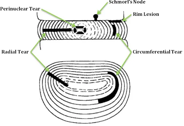
Annular defects have been categorized into classic tear categories: radial,

circumferential, perinuclear (Osti, Vernon-Roberts et al. 1992, Vernon-Roberts,

Moore et al. 2007) and other defects such as rim lesions and Schmorl’s nodes (Figure

3). Radial tears typically initiate at the NP and radiate outward, occurring primarily

(25)

11

increased age (Osti, Vernon-Roberts et al. 1992, Vernon-Roberts, Fazzalari et al.

1997). Circumferential tears are the separation of lamellae and occur equally in the

anterior and posterior AF, often concentrated in the outer regions (Osti,

Vernon-Roberts et al. 1992, Vernon-Vernon-Roberts, Fazzalari et al. 1997). Perinuclear tears are the

separation of the NP from the AF and result in a cleft (Vernon-Roberts, Moore et al.

2007).

In cadaveric studies, morphological/histological sections and discograms

(fluid contrast injected into the NP) have been used to quantify AF tears.

Morphological sections are limited because they only view one disc slice, while tears

occur in a complex 3D pattern (Vernon-Roberts, Fazzalari et al. 1997, Videman and

Nurminen 2004).

Figure 3: Representative annular and intervertebral disc defects. (Vernon-Roberts, Moore et al. 2007)

Discogram studies detect the presence of radial tears, but not their size or structure,

(26)

12

Kakitsubata, Theodorou et al. 2003, Videman and Nurminen 2004). The risk of a

radial AF tears has been shown to be 60% in early adulthood and 100% by

retirement age through an extensive discogram study of 157 cadaver spines. The

risk of a full AF tear is 10% for 20 to 49 year olds and 35% for 50 to 59 year olds

(Videman and Nurminen 2004). A comprehensive recent study using multiple

histological sections of L4-L5 quantified the incidence concentric tears to be ~100%

between ages 10 and 80 years (Vernon-Roberts, Moore et al. 2007). The incidence of

perinuclear tears was also high at ~90% across all ages. Posterior radial tears

increase from 70% incidence in those 10-30 years to 85% within the 51-89 year

group (Vernon-Roberts, Moore et al. 2007). Rim lesions occur at the junction of the

AF and vertebral endplate and are related to trauma, rather than degeneration. Rim

lesion data shows 30% incidence at age 30 and 90% at age 80 (Vernon-Roberts,

Moore et al. 2007). Schmorl’s nodes are herniations of the disc into the VB (Resnick

and Niwayama 1978). Reported frequency in the literature is varied (Hilton, Ball et

al. 1976, Hansson and Roos 1983, Hamanishi, Kawabata et al. 1994, Stabler, Bellan

(27)

13

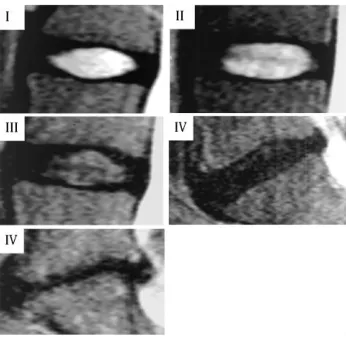
Figure 4: Pfirmann grading scale displaying degenerative changes visualized in MR (Pfirrmann, Metzdorf et al. 2001).

The degenerative IVD structural and compositional changes can be visualized

with MR imaging. Images illustrate a decrease in signal intensity, disc height narrowing,

and osteophytes on the vertebral bodies (Pfirrmann, Metzdorf et al. 2001). Pfirrmann et

al. established a qualitative graded scale (Figure 4) of increasing degeneration, where

non-degenerate discs are grades I-II, moderately degenerate are grades III-IV, and

severely degenerate grade V (Pfirrmann, Metzdorf et al. 2001).

Figure 5: T2 correlations to T1ρ and Pfirrmann from Elliot Lab lumbar spine database collected over several years for a multitude of studies

Since degeneration is a continuous process, quantitative MR mapping techniques

(28)

14

proteoglycan content (Blumenkrantz, Zuo et al. , Borthakur, Maurer et al. , Marinelli,

Haughton et al. , Takashima, Takebayashi et al. , Welsch, Trattnig et al. , Zuo, Joseph et

al. , Blumenkrantz, Li et al. 2006, Johannessen, Auerbach et al. 2006, Perry, Haughton et

al. 2006, Watanabe, Benneker et al. 2007, Nguyen, Johannessen et al. 2008, Marinelli,

Haughton et al. 2009). T2 mapping will be used within this study because it is more

repeatable and is correlated to both Pfirrmann grade and T1ρ score (Figure 5)

(Blumenkrantz, Zuo et al.).

2.5. Internal Deformations

Internal deformations of IVD strains have been measured through various optical

and radiographic techniques (Seroussi, Krag et al. 1989, Meakin and Hukins 2000,

Kusaka, Nakajima et al. 2001, Meakin, Redpath et al. 2001, Tsantrizos, Ito et al. 2005,

Ho, Kelly et al. 2006, Costi, Stokes et al. 2007). Physical markers were inserted to track

displacements within the disc. Markers included metal beads (Seroussi, Krag et al. 1989),

thin wires (Tsantrizos, Ito et al. 2005, Costi, Stokes et al. 2007), or nylon rods (Kusaka,

Nakajima et al. 2001). These markers offered limited accuracy since they were able move

separately from the structure of the disc. This limitation was improved by the use of

Alcian blue stain dots to track the displacements of a sagittaly bisected disc against

transparent Plexiglas (Meakin and Hukins 2000, Meakin, Redpath et al. 2001, Ho, Kelly

et al. 2006); however, bisection depressurizes the disc. The recent application of the

commercial texture correlation software Vic2D (Correlated Solutions Inc: Columbia, SC)

(29)

15

in 2D within the sagittal and coronal plane of the disc (O'Connell, Malhotra et al. ,

O'Connell, Vresilovic et al. , O'Connell, Johannessen et al. 2007).

O’Connell et al. utilized a turbo spin echo (TSE) with TR/TE = 3000/113 ms

respectively, producing T2-weighted 2D mid-sagittal/coronal MR images with in-plane

resolution of 234 μm/pixel and 3mm slice thickness on a 3T clinical MRI scanner

(O'Connell, Johannessen et al. 2007). Spin-echo based sequences have been widely used

for MR imaging of the intervertebral disc (Haughton 2004) because they are less

susceptible to inhomogeneity’s in the magnetic field. T2-weighting an image with a long

echo time (TE) and long repetition time (TR) provides brighter signal for high water

content soft tissues and darker for fat predominant tissues. Texture correlation strain

measurements (resolution of 1/20th pixel = 11.7μm) were validated against displacement

measurements across the entire disc and also against finite element studies (O'Connell,

Johannessen et al. 2007). Under axial compression it was found that compressive and

radially tensile strains increased with degeneration (O'Connell, Vresilovic et al.). The

posterior AF experienced the highest regional strain and did not correlate with

degeneration, indicating that the posterior region undergoes high loads throughout life

(O'Connell, Vresilovic et al.). The use of MRI to measure internal deformations permits

the study of clinical treatments such as nucleotomy, which increases compressive AF

strains while decreasing radial strain (O'Connell, Malhotra et al.). Despite significant

technical improvements, these studies are limited to 2D strain measurements for a 3D

structure. It is difficult to limit out of plane motion; the 3D techniques developed in this

thesis will mitigate these limitations. Texture correlation has been shown to produce

(30)

16

MR images (Gilchrist, Xia et al. 2004). Recognition of such limitations has directed the

implementation of image registration to perform strain analysis on medical images

(Phatak, Sun et al. 2007). This process produces comparable results to texture correlation

(Hardisty, Akens et al. , Villemure, Cloutier et al. 2007). A non-rigid image registration

method was employed by Reiter et al. to calculate mid-sagittal strain after creep loading

(Reiter, Fathallah et al. 2012). Displacement encoded MRI, an image tagging method that

enables direct displacement measurements from MR data, was used by Chan and Neu to

calculate strain across the entire disc under cyclic loading (Chan and Neu 2013). These

studies utilized MR phantoms (Chan and Neu 2013) or computer generated deformations

(Reiter, Fathallah et al. 2012) to verify strain measurements. However, experimental

specific verification can provide a better sense of what is actually occurring within the

disc (ground truth). Image registration and the application of overlap statistics with

segmentations will provide strain analysis of the entire disc and accurate disc-specific

reportable strain resolution in Chapter 6-8.

2.6. Medical Image Analysis and Registration Applications

Quantitative image analysis including texture correlation, digital volume

correlation and image registration (Liang, Zhu et al. , O'Connell, Malhotra et al. ,

O'Connell, Vresilovic et al. , Tustison, Cook et al. , Weiss, Rabbitt et al. 1998, Bay,

Smith et al. 1999, Bay 2001, Veress, Weiss et al. 2002, Tustison, Davila-Roman et al.

2003, Veress, Gullberg et al. 2005, Tustison and Amini 2006, Chandrashekara,

Mohiaddin et al. 2007, Liu and Morgan 2007, O'Connell, Johannessen et al. 2007,

(31)

17

extensively used to measure strain from various biomedical imaging modalities. Texture

correlation is a pattern-matching algorithm that compares random patterns of pixel

intensities between two images, calculating displacements between individual pixels in

corresponding images. Digital volume correlation is an adjunct to digital image

correlation, a form of texture correlation utilizing 3D images to track microstructural

feature movement within specimens (Bay, Smith et al. 1999, Bay 2001, Liu and Morgan

2007). Image registration is the process of finding a transformation (warp field) which

can map points from a reference image (original) to a different image (deformed) (Ng and

Ibanez 2004), this technique has been widely applied to medical images.

Image registration permits various imaging modalities, including X-Ray, CT, and

MRI which can be spatially aligned to correlate data (Maintz and Viergever 1998). The

wide applicability of image registration enables physicians to quantitatively detect subtle

changes between images, facilitate identification and localization of brain lesions for

surgical guidance (Ng and Ibanez 2004), assess treatment effectiveness pre- and post-

intervention and tumor/disease development (Maintz and Viergever 1998, Ng and Ibanez

2004), hippocampus disease valuation via template building for population studies

(Avants, Yushkevich et al.), and measuring ligament, pulmonary, and cardiovascular

tissue mechanics (Liang, Zhu et al. , Tustison, Cook et al. , Weiss, Rabbitt et al. 1998,

Veress, Weiss et al. 2002, Tustison, Davila-Roman et al. 2003, Veress, Gullberg et al.

2005, Tustison and Amini 2006, Chandrashekara, Mohiaddin et al. 2007, Phatak, Sun et

al. 2007, Phatak, Maas et al. 2009, Tustison, Avants et al. 2009). Parameter selection is a

critical process when performing image registration in a new tissue, in Chapter 6-7 these

(32)

18

2.7. Advanced Normalization Tools Image Registration Parameters

Registrations are performed using either features or image intensity. Features

include specific points and landmarks or binary structures within the native anatomy,

which can be segmented as curves, surfaces, or volumes. Image intensity refers to the

image grayscale patterns. Landmark- and segmentation- based registration methods align

images, minimizing the distance between features. Intensity-based registrations minimize

a cost function that measures the similarity of the intensity between corresponding

images (Ng and Ibanez 2004). Advanced Normalization Tools (ANTs) is a

multi-resolution approach encompassing landmark-, segmentation-, and intensity- based

registration techniques.

The registration process is guided by 3 main parametric variables: transformation

model, regularization technique, and the similarity metric to define the resultant warp

field (Figure 6). The transformation model determines how one image is mapped into or

aligned with another image. Multiple transformation models exist to account for varying

degrees of differentiation between the images registered. During registration, ANTs has

the ability to account for rigid translation and rotation to align one image with another.

Deformable or non-rigid models (Diffeomorphic or Elastic) are more flexible, modeling

and deforming the image as a continuum (e.g. elastic material, viscous fluid, etc.) (Avants

and Gee 2004). During registration, the transformation model deforms the images on an

overlaid grid or warp field. Generally, points that fall along gridlines are matched directly

to points in the second image, and thus the grayscale intensity is known. The

regularization technique interpolates the pixel intensity of points mapped between

(33)

19

Gonner et al. 1999, Tustison, Avants et al. 2009) interpolators, which use Gaussian

distributions and basis functions respectively, to assign intensity values. The choice of

regularization as well as its measures (e.g. size of variance and number of splines) affects

the smoothness of the mapping. Similarity metrics are statistical measures used to

quantify the resemblance between the pixel intensity patterns in both images. Different

statistical measures should be used if pixel intensities and patterns are consistent or vary

across images. The metric choice is thus dependent on whether one or multiple imaging

modalities are used. ANTs offers several similarity metrics and is capable of both mono-

and multi- modality registrations. Mean squared difference (MSQ) and fast cross

correlation (CC) are ideal for mono-modality registrations, which are employed in this

work.

(34)

20

CHAPTER 3 Cartilaginous Endplate Geometry

3.1. Introduction

The intervertebral disc has three distinct anatomical regions: the central nucleus

pulposus (NP), the surrounding annulus fibrosus (AF), and centrally positioned

cartilaginous endplates (CEP). These CEPs are distinct from the adjacent vertebral

endplates, which are composed of cortical bone (Francois, Bywaters et al. 1985, Roberts,

Menage et al. 1989, Raj 2008). The CEP is an approximately 600 μm thick layer of

hyaline cartilage positioned between the vertebral endplate and NP (Roberts, Menage et

al. 1989). It functions both as a mechanical barrier between the pressurized NP and the

vertebral bone, as well as a gateway for nutrient transport into the disc from adjacent

blood vessels (Crock and Goldwasser 1984, Roberts, Menage et al. 1993, Moore 2000,

Urban and Roberts 2003).

Intervertebral disc degeneration causes the CEP to become sclerotic, lose vascular

contact, and exhibit decreased permeability (Nachemson, Lewin et al. 1970, Bernick and

Cailliet 1982, Roberts, Urban et al. 1996, Grignon, Grignon et al. 2000, Bibby, Jones et

al. 2001, Benneker, Heini et al. 2005, Accadbled, Laffosse et al. 2008). This process is

considered to contribute to degeneration by reducing diffusion of nutrients to cells of the

NP (Ariga, Miyamoto et al. 2001, Martin, Boxell et al. 2002, Adams and Roughley 2006,

Raj 2008).

The literature is replete with cadaveric studies using histology or gross sections

depicting CEP thickness (Roberts, Menage et al. 1993, Vernon-Roberts, Fazzalari et al.

1997, Videman and Nurminen 2004, Bae, Statum et al. 2013). However, even multiple

(35)

21

accurate quantitative techniques for characterization of the 3D human CEP. Magnetic

resonance imaging (MRI) is a non-invasive, non-ionizing imaging modality well known

for its superior soft tissue contrast, making it ideal for disc applications including

anatomy, composition, and stage of degeneration through a number techniques (e.g., T1ρ-

and T2-weighted images) (Lyons, Eisenstein et al. 1981, Pfirrmann, Metzdorf et al. 2001,

Antoniou, Mwale et al. 2006, Johannessen, Auerbach et al. 2006). Application of MRI to

the study of the intervertebral disc has to date focused predominantly on the composition

of the NP and AF. Few studies have examined the CEP, therefore the objective of this

chapter is to develop MRI techniques to visualize and quantify the CEPs geometric.

In-order to visualize the thin CEP and accurately measure is thickness, a sufficiently high

(36)

22

3.2. Materials and Methods

3.2.1. Intervertebral disc MRI parameter measurement

In this chapter, a T1weighted 3D FLASH (fast low-angle shot) sequence was

chosen for CEP imaging. In the FLASH sequence, transverse magnetization is spoiled

and the steady-state longitudinal magnetization depends on T1 and the flip angle. Flip

angle is the angle at which the net magnetization is rotated relative to the primary

magnetic field (B0) by application of an excitation pulse. The sequences parameters

repetition time (TR) and flip angle thus determine the T1 contrast in the FLASH

sequence and were optimized in this study using an analytical model. Repetition time

(TR) is the amount of time between successive pulses applied during image acquisition.

Optimized sequence parameters TR and flip angle will yield sufficient image contrast to

distinguish the CEP from its adjacent tissue.

The first step in MR image sequence optimization involves determining the MRI

tissue specific properties. To achieve a T1 weighted image, the T1 relaxation time must

be determined. T1 relaxation time (measured in milliseconds) known, as longitudinal

relaxation time is a measure of the time required for a tissues protons to realign with B0.

T1 values of NP, CEP, and AF lamellae were measured in a representative healthy and

degenerate cadaveric lumbar disc (Grade = 2.3/5) (Pfirrmann, Metzdorf et al. 2001) at 7T

magnetic field strength. T1 was measured using a fully relaxed (TR = 5100 ms) 2D spin

echo inversion recovery pulse sequence with ten inversion times (TI = 33 – 5000 ms). T1

maps were generated (Figure 7) by fitting data on a pixel-by-pixel basis to its respective

(37)

23

Equation 1). Averaging 900 or more pixels within center of the NP, anterior and posterior

AF, and CEP determined representative T1 values of each disc substructure.

Equation 1:

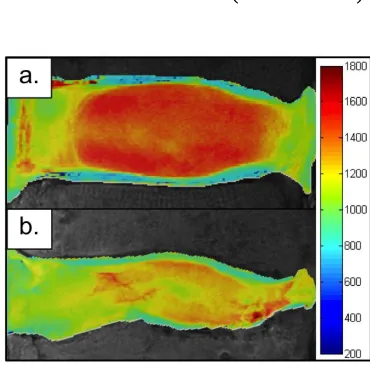
Figure 7: Representative T1 parameter maps at 7T: (A) T1 healthy, (B) T1 degenerate

3.2.2. Optimization of CEP image contrast

In order to attain pulse sequence parameters with optimized contrast in the CEP,

MRI signal intensity and image contrast were simulated using an analytical MRI pulse

sequence equation prior to imaging. The T1 contrast of the FLASH sequence is a

function only of TR and flip angle in the limit of a short echo time (TE), and the

dependence of MRI signal intensity upon flip angle, TR, and T1 is given by Equation 2

where A is the equilibrium magnetization reduced by T2 relaxation and α is the flip angle

(Helms, Dathe et al. 2008, Dathe and Helms 2010). Echo time (TE) corresponds to the

time between RF pulse and the peak in signal. T2 relaxation time known, as transverse

relaxation is a measure of time required for a tissues protons to dissipate energy to their

surrounding nuclei perpendicular to B0.

(38)

24

This equation was used to analyze the signal dependence on flip angle and TR, the

primary adjustable imaging parameters in this application. Using the experimentally

determined mean T1 and I0 values for NP and CEP, normalized MRI signals (

Equation 2) for each substructure were plotted versus flip angle and TR. The image

contrast (signal difference) between NP and CEP (

Equation 3), normalized to maximize the signal intensity of CEP, was plotted versus flip

angle and TR for the full range of possible parameter values according to ex vivo MR

imaging

Equation 3:

3.2.3. Cartilaginous Endplate Imaging

Specimens for CEP imaging were prepared from 11 cadaveric human lumbar spines

(n = 17 discs, age: 57.7 ± 13.3). While for some subjects 2–3 levels were used from a

single spine, consistent with common practice in the literature (O'Connell, Vresilovic et

al. , Iatridis, Setton et al. 1997, Rodriguez, Slichter et al. 2011), these discs were assumed

to be independent samples and post hoc statistical analysis confirmed no subject

dependence on CEP height. Each whole spine was first scanned with a mid-sagittal T2-

weighted turbo spin echo imaging sequence for routine grading of degenerative state

(Pfirrmann, Metzdorf et al. 2001, Johannessen, Auerbach et al. 2006). The integer grade

from five individual examiners was averaged (Grade: 2.8 ± 0.7). Lumbar spines were

then dissected into bone-disc-bone segments with posterior elements removed and sealed

in airtight freezer bags to avoid dehydration during imaging. The sealed segments were

then embedded in 2 % agarose gel for immobilization and to reduce image distortion at

(39)

25

For protocol optimization, the flip angle and TR that provided the best optimal

NP-CEP contrast was selected using the analytical model simulation. All imaging was done

in a Siemens Magnetom 7T scanner (Siemens Medical Solutions, Erlangen, Germany)

using a 4-channel ankle coil (Insight MRI) (Wright, Lemdiasov et al. 2011). Due to the

thinness of the endplate, a voxel size of 200 μm3 was chosen. Imaging parameters were

TR = 9 ms, TE=3.7ms, flip angle=20°, (0.2 mm)3isotropic resolution, matrix = 320 x

320, and fat suppression. Scan time was 3 min per disc.

3.2.4. CEP Histology and endplate thickness quantification

Histological analysis was performed to confirm that the structure visualized using

MRI was indeed the CEP and to compare CEP thickness measurements with

measurements from site-matched MR images. Two adjacent 8 mm biopsy punches,

comprising vertebral bone, the CEP and the NP, were taken from a disc (63 years, male,

L2L3, Grade: 2.6), which had previously been imaged as described above, and an optical

image of the specimen was taken. These 200 μm3 isotropic MRI data and photograph

were later co-registered to confirm the location of the punches. Both punches were fixed

in buffered 10% formalin overnight. One punch was then decalcified overnight in formic

acid/EDTA. Twenty-micron sections were cut on a cryostat, and double stained with

Alcian blue and picrosirius red to demonstrate glycosaminoglycans and collagen,

respectively, and imaged using bright field microscopy. The other punch was sectioned in

a similar way, but without prior decalcification. These sections were then stained using

the von Kossa method to demonstrate calcium deposits and imaged using differential

(40)

26

To compare MRI-based CEP measurements with a histological standard, three 4

mm diameter CEP samples were punched within the inferior endplate for a single disc

(75 years, male, L2L3, Grade: 2.0), sectioned on a cryostat, and the CEP thickness

measured at three evenly spaced intervals across the plug. Virtual plugs were generated

from the MR data by co-registering with an optical image of the vertebral surface and

site-matched CEP thickness measurements were made.

Images were imported into OsiriX software and evaluated for CEP contrast in

comparison to the surrounding structures, for morphology three dimensions thickness.

MRI data had isotropic resolution and, therefore, could be viewed in arbitrary image

planes using multi-planar reformatting. The CEP thickness was measured for the superior

and inferior CEP along the mid-sagittal plane at five locations (center, 5 and 10 mm off

the center towards anterior and 5 and 10 mm off the center towards posterior). Average

thicknesses across specimens were measured by hand within OsiriX for each location and

each disc level.

The CEP thickness measurements were evaluated using a two-way ANOVA with

repeated measures, where the factors were disc level (L1L2, L2L3, L3L4, L4L5, L5S1)

and anterior-posterior disc location (center, 5 and 10 mm off the center towards anterior,

and 5 and 10 mm off the center towards posterior). Significance was set at p < 0.05. A

post hoc Bonferonni test was performed when significance was detected resulting in

(41)

27

3.3. Results

Average T1 values (±standard deviation) from the T1 parameter map (Figure 7) of

each disc substructure obtained at 7T are presented for a representative healthy and

degenerate disc substructures in Table 1. These T1 values were used in Equation 2 and

Equation 3 to calculate signal intensity and determine optimal pulse sequence parameters

for NP-CEP image contrast (DCEP) (Figure 8). Figure 8a shows a contour plot of DCEP

covering the exhaustive range of flip angles (0–180°) and TR values (0–6,000 ms).

However, only a small region corresponding to short TR (dotted box in Figure 8a), where

scan time is reasonable for future in vivo applications, was considered in selecting the

optimal sequence parameters (Figure 8b), and the optimal flip angle and TR were

identified (asterisk in Figure 8b).

Grade Region T1

Healthy

AF 1270 ± 80

NP 1510 ± 50

CEP 775 ± 75

Degenerate

AF 1100 ± 43

NP 1300 ± 65

CEP 840 ± 32

Intervertebral Disc Structure and Mechanical Function Under Physiological Loading Quantified Non-invasively Utilizing MRI and Image Registration

ScholarlyCommons

Intervertebral Disc Structure and Mechanical

Function Under Physiological Loading Quantified

Non-invasively Utilizing MRI and Image

Registration

Intervertebral Disc Structure and Mechanical Function Under

Physiological Loading Quantified Non-invasively Utilizing MRI and

Image Registration

INTERVERTEBRAL DISC STRUCTURE AND MECHANICAL

FUNCTION UNDER PHYSIOLOGICAL LOADING QUANTIFIED

NON-INVASIVELY UTILIZING MRI AND IMAGE

REGISTRATION

Jonathon Henry Yoder

ABSTRACT

Table of Contents

List of Tables

List of Illustrations

CHAPTER 1

Introduction

CHAPTER 2

Background

2.1.

Clinical Significance

2.2.

Intervertebral Disc Structure

2.3.

Disc Mechanical Function

2.4.

Disc Degeneration

2.5.

Internal Deformations

2.6.

Medical Image Analysis and Registration Applications

2.7.

Advanced Normalization Tools Image Registration Parameters

CHAPTER 3

Cartilaginous Endplate Geometry

3.1.

Introduction

3.2.

Materials and Methods

3.3.

Results