Family Algebras and the Isotypic Components of g tensor g

(1)

University of Pennsylvania

ScholarlyCommons

Publicly Accessible Penn Dissertations

1-1-2014

Family Algebras and the Isotypic Components of g

tensor g

Matthew Tai

University of Pennsylvania, mtai@sas.upenn.edu

Follow this and additional works at:

http://repository.upenn.edu/edissertations

Part of the

Mathematics Commons

This paper is posted at ScholarlyCommons.http://repository.upenn.edu/edissertations/1464

For more information, please contactlibraryrepository@pobox.upenn.edu.

Recommended Citation

(2)

Family Algebras and the Isotypic Components of g tensor g

Abstract

Given a complex simple Lie algebra $g$ with adjoint group $G$, the space $S(g)$ of polynomials on $\mg$ is isomorphic as a graded $\mg$-module to $(I(g)\otimes \mathscr{H}(g)$ where $I(g) = (S(g))^G$ is the space of $G$-invariant polynomials and $\mathscr{H}(g)$ is the space of $G$-harmonic polynomials. For a representation $V$ of $g$, the generalized exponents of $V$ are given by $\sum_{k \geq

0}dim(Hom_g(V,H_k(g))q^k$. We define an algebra $C_V(g) = Hom_g(End(V),S(g))$ and for the case of $V = g$ we determine the structure of $g$ using a combination of diagrammatic methods and information about representations of the Weyl-group of $g$. We find an almost uniform description of $C_g(g)$ as an $I(g)$-algebra and as an $I(g)$-module and from there determine the generalized exponents of the

irreducible components of $End(g)$. The results support conjectures about $(T(g))^G$, the $G$-invariant part of the tensor algebra, and about a relation between generalized exponents and Lusztig's fake degrees.

Degree Type

Dissertation

Degree Name

Doctor of Philosophy (PhD)

Graduate Group

Mathematics

First Advisor

Alexandre Kirillov

Keywords

Associative Algebras, Generalized Exponents, Lie Theory, Representation Theory

Subject Categories

(3)

FAMILY ALGEBRAS AND THE ISOTYPIC COMPONENTS OF

g

_⊗

g

Matthew Tai

A DISSERTATION

in

Mathematics

Presented to the Faculties of the University of Pennsylvania

in

Partial Fulfillment of the Requirements for the

Degree of Doctor of Philosophy

2014

Supervisor of Dissertation

Alexandre Kirillov

Professor of Mathematics

Graduate Group Chairperson

David Harbater

Professor of Mathematics

(4)

Acknowledgments

I would like to thank Professor Alexandre Kirillov, my advisor, for both suggesting the

problem to me and for providing supervision and insight.

I would also like to thank Professors Wolfgang Ziller, Tony Pantev, Siddhartha Sahi, Jim

Lepowsky, Yi-Zhi Huang, Roe Goodman, Dana Ernst, Christian Stump and Richard

Green for advice, encouragement and inspiration.

Special thanks to Dmytro Yeroshkin for tremendous help, mathematically and

compu-tationally, and for listening to me complain about notation. I would also like to thank

his father Oleg Eroshkin for additional suggestions to ease computing.

Thanks as well to my friends and colleagues here at the UPenn math department, for

(5)

ABSTRACT

FAMILY ALGEBRAS AND THE ISOTYPIC COMPONENTS OFg⊗g

Matthew Tai

Alexandre Kirillov

Given a complex simple Lie algebragwith adjoint groupG, the spaceS(g) of

poly-nomials ongis isomorphic as a gradedg-module to (I(g)⊗H(g) whereI(g)=(S(g))G

is the space ofG-invariant polynomials and H(g) is the space of G-harmonic

poly-nomials. For a representation V of g, the generalized exponents of V are given by

X

k≥0

d i m(Homg(V,Hk(g))qk. We define an algebraCV(g)=Homg(End(V),S(g)) and

for the case ofV =gwe determine the structure ofgusing a combination of

diagram-matic methods and information about representations of the Weyl-group of g. We

find an almost uniform description ofCg(g) as anI(g)-algebra and as anI(g)-module

and from there determine the generalized exponents of the irreducible components

ofEnd(g). The results support conjectures about (T(g))G, theG-invariant part of the

tensor algebra, and about a relation between generalized exponents and Lusztig’s fake

(6)

List of Tables

1.1 Exponents for the simple Lie algebras . . . 2

6.1 Generalized Exponents inC_ω₁₊_ω_r(Ar) . . . 42

6.2 Generalized Exponents inC_ω₁₊_ω₃(A3) . . . 43

7.1 Generalized Exponents inCg(Br/Cr) . . . 55

7.2 Generalized Exponents inCg(B3/C3) . . . 55

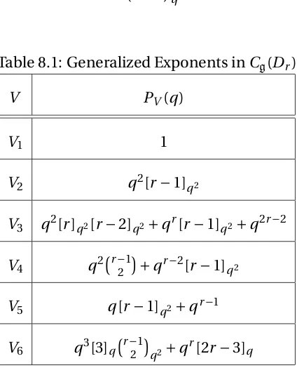
8.1 Generalized Exponents inCg(Dr) . . . 64

8.2 Generalized Exponents inCg(D3) . . . 65

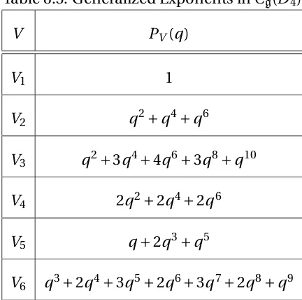
8.3 Generalized Exponents inCg(D4) . . . 66

9.1 Generalized exponents as fake degrees forAr . . . 69

9.2 Generalized exponents as fake degrees forBCr . . . 69

9.3 Generalized exponents as fake degrees forDr . . . 70

10.1 Exponents for the Exceptional Lie algebras . . . 75

(10)

11.1 Generalized Exponents inCg(G2) . . . 85

12.1 Fake degrees inEnd(F4)T . . . 89

12.2 Generalized Exponents inCg(F4) . . . 93

13.1 Fake degrees inEnd(E6)T . . . 96

13.2 Generalized Exponents inCg(E6) . . . 98

14.2 Generalized Exponents inCg(E7) . . . 103

(11)

Chapter 1 Introduction

1.1 Simple Lie Algebras and Exponents

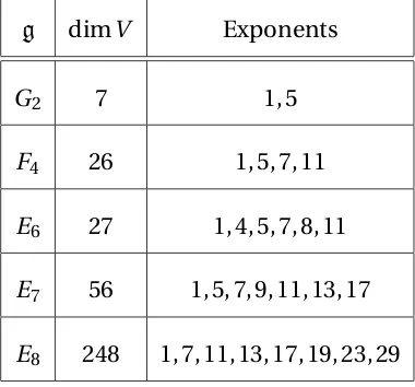
We consider the simple Lie algebras, these being the four classical seriesAr,Br,Cr,Dr

and the five exceptional algebrasG2,F4,E6,E7,E8. Associated to each of these algebras

is a list of numbers called their exponents, which appear in a number of ways. The

name comes from the exponents of the hyperplane arrangement corresponding to the

simple reflection planes of the Weyl Group of the Lie algebra. The exponents can also

be considered topologically: for the compact group G associated tog, the Poincare

polynomial ofGis

PG(q)=

X

k=0

r k(Hk(G,Z))qk=

r

Y

k=1

(1+q2ek+1)

The simple Lie algebras are summarized in the following table, where the descriptions

(12)

Table 1.1: Exponents for the simple Lie algebras

g dimg Exponents Notes

Ar r2+2r 1, 2, 3 . . . ,r sl(r+1)

Br r(2r+1) 1, 3, 5, . . . , 2r−1 so(2r+1)

Cr r(2r+1) 1, 3, 5, . . . , 2r−1 sp(r)

Dr r(2r−1) 1, 3, 5, . . . , 2r−1,r−1 so(2r)

G2 14 1, 5 “sl(1,O)00

F4 52 1, 5, 7, 11 “sl(2,O)00

E6 78 1, 4, 5, 7, 8, 11 “sl(2,C⊗O)00

E7 133 1, 5, 7, 9, 11, 13, 17 “sl(2,H⊗O)00

(13)

1.2 Casimir Invariants

The exponents ofgalso have representation-theoretic interpretations.Gacts ongvia

the conjugation action, and hence onS(g), the symmetric algebra ongconsidered as

a vector space. We denote byI(g) theG-invariant subspace (S(g))G. In 1963, Kostant

showed thatI(g) for simplegis a polynomial algebra where the number of generators

is equal to the rank ofg, and that furthermore the degrees of these generators are each

one more than an exponent ofg. For later use we establish a particular choice of

gen-erators ofI(g), which we will call primitive Casimir operators.

For each Lie algebra, we pick a representation (V,π) with which to define the primitive

Casimir operators. Forsl(r+1) we pick one of the twor+1-dimensional

representa-tions. Forso(n) we pick then-dimensional representation, and forsp(r) we pick the

2r-dimensional representation. ForG2,F4,E6,E7, andE8we pick the 7−, 26−, 27−, 56−,

and 248−dimensional representations respectively. These are often also called the

“standard” representations, and with a few exceptions are the nontrivial

representa-tions of minimal dimension. From here on out, unless otherwise specified, V andπ

refer to this defining representation.

Letting {x_α} be a basis ofgandK be the Killing form, define

Md=π(xα)⊗Kαβxβ

regarded as anS(g)-valued square matrix of dimension dimV.

(14)

we can denote the exponents by

e1<e2<. . .<er

We define the Casimir operator

ck=t r(M_dek+1)

where the trace is taken in the minimal representationV. The set {ck} are the primitive

Casimir operators forg.

In the case ofDr, the exponents are 1, 3, . . . , 2r−3,r−1. We order the exponents in

increasing order, getting thate_dr

2e =r−1. Fork6=

§_r

2

¨

, we write

ck=t r(M_dek+1)

and fork=§r₂¨we define

ck=P f =

p

det(Md)

picking the sign ofP f arbitrarily.

Forsl(r+1), the exponents areei=ifor 1≤i≤r. Fork>r+1, we have the reduction,

0= X

njmj=k

1

mj!

Ã

−t r(M

nj

d )

nj

!mj

where the notationnjmj =kindicates a partition ofk wherenj appears with

multi-plicitymj. In particular, the relation fork=r+2 is the trace of the Cayley-Hamilton

identity forMd.

(15)

k not an exponent plus 1, with varying complexity. For the exceptional Lie algebras,

dim(V) is much larger thaner+1, so the Cayley-Hamilton identity doesn’t yield much

information about the how traces of low powers ofMd reduce. See [RSV99] for details.

1.3 Generalized Exponents

In 1963, Kostant [Ko63] proved that for a representationV ofgand hence ofG, (V⊗

S(g))G=HomG(V∨,S(g)) is a freeI(g) module. Thus we can find a basis for (V⊗S(g))G

overI(g); Kostant calls the degrees of the polynomial components of this basis the

gen-eralized exponents ofV (with multiplicity), usually expressed as a polynomialPV(q)

for a variableq. Note that forV =g, the generalized exponents forgmatch the

classi-cal notion of the exponents ofg.

There is another description of the generalized exponents in terms of a spaceH(g) of

G-harmonic polynomials. LetD(g) be the space ofG-invariant differential operators

onS(g) with constant coefficients, and letD₊(g) be the subspace ofD(g) with

vanish-ing constant term. ThenH(g) is defined by

H(g)={f ∈S(g)|d(f)=0∀d∈D₊(g)}

The conditiond(f)=0 generalizes the usual harmonic condition of∆(f)=0, and thus

theG-harmonic polynomials allow for studying functions defined on Lie groups using

methods from harmonic analysis.

(16)

I(g) are invariant, all of the interesting behavior is contained inH(g). Thus we can

write the generalized exponents of a representationV as

PV(q)=

X

k

dim(Homg(V,Hk(g)))qk

Hesselink [He80] gives a formula for computing the generalized exponents of an

irre-ducible representation of a simple Lie algebra using aq-analogue of Kostant’s

multi-plicity formula, but using this formula is computationally infeasible, involving

com-puting the q-analogue of the partition function, which unlike the normal partition

function doesn’t vanish for negative weights, and then summing the partition

func-tion over the associated Weyl orbit. There are also combinatorial approaches such as

the Kostka-Foulkes polynomials forsl(n) [DLT94]. For representations where none of

the weights are twice a root (called small representations), Broer [Br95] showed that

the generalized exponents ofV are equal to what Lusztig calls the fake degrees [Lu77]

ofVT as a representation ofW.

In general, however, there are no known closed-form expressions for the generalized

exponents of arbitrary representations that don’t require summation over the Weyl

(17)

Chapter 2 Introduction to Family Algebras

2.1 Definition of Family Algebras

In [Ki00], Kirillov introduced what he calls Family Algebras in the hopes of providing

a new method for determining generalized exponents that doesn’t involve summing

over the Weyl group.

We fix a representationV ofgand considerEnd(V), with the conjugation action on it

induced from the action onV. We define the classical family algebra

CV(g)=(End(V)⊗S(g))G

whereG is the adjoint group ofg and acts by the action induced fromg. This is an

algebra with multiplication◦ ⊗minherited from

(18)

via composition and

m:S(g)⊗S(g)→S(g)

via polynomial multiplication.

If we pick a basis {va} forV and letEabbe defined byEabvb=va, then we can write an

element of the family algebra as

E_ab⊗P_ba

whereP_ba∈S(g). We call the set {P_ba} the polynomial component ofE_ab⊗P_ba. Note that

for two elementsEb_a⊗P_baandEb_a⊗Qa_b, the multiplication looks like

(E_ab⊗P_ba)×(Eb_a⊗Qa_b)=Eb_a⊗P_caQc_b

So the multiplication respects the natural grading on the polynomial components, and

hence we say that an elementEb_a⊗P_bais homogeneous of degreekif all of the {P_ba} are

homogeneous of degreek.

The phrase “family algebra” comes from the decomposition of

End(V)=M

i

Vi

for irreducibleVi, which Kirillov calls the children ofV. The family algebraCV(g)

de-composes similarly into

CV(g)=

M

i

(Vi⊗S(g))G

Thus a family algebra gives us anI(g) module that is closed under multiplication and

(19)

End(V), then so isV∨

i ; hence

CV(g)=

M

i

(Vi⊗S(g))G∼=

M

i

Homg(Vi,S(g))

There is a natural quantization to what Kirillov calls the quantum family algebra,

QV(g)=(End(V)⊗U(g))G

U(g) is isomorphic toS(g) asG-modules, so there is a map that sendsQV(g) toCV(g),

but the classical and quantum family algebras for a givenV differ in their

multiplica-tive structures. This dissertation will only consider classical family algebras.

2.2 Relation to the Generalized Exponents

For an irreducible representation Vi, there is an I(g)-linear basis of Homg(Vi,S(g))

where there is a bijection between generalized exponentsei j (with multiplicity) and

basis elementsAi j such that

Ai j∈Homg(Vi,Hei j(g))

Hence, using the decomposition ofEnd(V) into irreducible representations, there is

anI(g)-linear basis ofCV(g) where each basis element is inHomg(Vi,Hei j(g)) for some

Vi in the decomposition ofEnd(V) and someei j a generalized exponent ofVi.

Thus the general strategy of family algebras is to determine the algebraic structure of

a given family algebra, use that to determine anI(g)-linear basis, turn that basis into a

(20)

2.3 Restriction to the Cartan subalgebra

Given a Cartan subalgebrahofgwith corresponding torusT ⊂G, we can look atS(h),

and in particular the restrictionr es:S(g)→S(h) given by viewing the two algebras as

Pol[g∨] andPol[h∨] respectively, and sending an element f ∈S(g) to f|h∨. While this

map is generally not an injection, there are some useful aspects. Chevalley’s restriction

theorem [Br95] says that

r es|I(g):I(g)→I(h)=S(h)W

is an isomorphism. We get a map

Res: (V⊗S(g))G→(VT⊗S(h))W

induced by restricting from V to VT and fromS(g) to S(h), which Kostant shows is

an injection. The result by Broer mentioned in the first chapter is a necessary and

sufficient condition forResto be an isomorphism.

WritingBV(h) forEnd(V)T⊗S(h) we get that

Res:CV(g)→BV(h)W

is an injection. We can make Res into a surjection by localizing with respect to the

non-zero part ofI(g). In particular, letK0be the fraction field ofI(g)∼=S(h)W. Then by

[Ki01] we have that

(21)

This then tells us that the dimension ofCV(g) over I(g) is equal to the dimension of

BV(h)W overI(h).

End(V)T = M

µ∈W t(V)

M atmV(µ)(C)

and soBV(h)W is theW-invariant subalgebra of the sum of matrix algebras

M

µ∈W t(V)

M atmV(µ)(S(h))

Since the multiplicity over I(h) of a representation φofW inS(h) is dim(φ), the

di-mension ofBV(h)W overI(h), i.e. the dimension ofCV(g), is given by the sum of the

dimensions of the matrix algebras:

X

µ∈W t(V)

mV(µ)2

Given a weightλ∈W t(V), we can consider an element ofBV(h)W that is the identity

on the matrix algebras corresponding to weights inW.λand vanish elsewhere. Such

an element lifts to an element ofCV(g) which, for someP∈I(h), restricts toPtimes the

identity on the matrix algebras corresponding to weights inW.λand vanish elsewhere.

(22)

Chapter 3 Results for

V

₌

g

This dissertation will focus on the particular case of the adjoint representation, i.e.

set-tingV =g. The weights in question are then the roots ofgas well as 0 with multiplicity

r, wherer is the rank ofg. We denote the image of (End(g)T⊗S(h))W inM atr(S(h)) by

the torus part of the algebra, and everything else by the vector part, as it is composed

of 1-dimensional and hence scalar algebras. Note that the vector part is commutative,

sinceS(h) is commutative, so any non-commutativity in the family algebra appears

only in the torus part.

3.1 Algebraic Structure

The decomposition ofEnd(g) into irreducible components depends ong, but is

uni-form for all of the An, uniform forBn,Cn andDn, and is uniform for the five

(23)

ofCg(g) as ag-module ends up quite different, the algebraic structures ofCg(g) are

very similar for all of the simple Lie algebras. There are two generators common to

all of family algebras in question, denotedM andS, and then a set ofr other

gener-ators, labelledR1throughRr, that depend on the structure ofg. A set ofI(g)-linearly

independent basis elements ofCg(g) is then

MmRkfor 0≤m≤er+1, 1≤k≤r

RmSRn+RnSRm for 1≤m≤n≤r−1

RmSRn−RnSRmfor 1≤m<n≤r

HereR1is a scalar, left in for uniformity of expression.

TheRk can themselves be generated by eitherM,S andR2 in the cases of Ar,Br,Cr

andG2, byM,S,R2andRr forDr, or byM,S,R2 andR3.in the cases ofF4,E6,E7and

E8.

There are several relations common to all of the cases. The terms MmRk for m≥1

vanish on the torus part, and any term involvingSvanishes on the vector part. Hence

M is central andM S =SM =0. TheRk commute with each other and withM, but

not with S. SRkS=PkS for some Pk ∈I(g), although the form of Pk depends on g.

The relations describing the products of the Rk also depend on g, in particular the

(24)

3.2 Fake Degrees

For the Weyl groupW acting on the Cartan subalgebrah, there is a notion called “fake

degrees” analogous to that of the generalized exponents, in that there is a

polyno-mialPU(q) describing the maps from aW-representationU into a spaceM(h) ofW

-harmonic polynomials. For the representations relevant tog⊗g, we have the following

statement: ifVT = ⊕iUi asW-modules, then

PV(q)=

X

i

qki_P

Ui(q)

for some set of exponentski, although theki are not uniquely determined.

For each classical families there are uniform expressions for the qi in terms of r, as

(25)

Chapter 4 Diagrams

We can write elements of the family algebra diagrammatically using the

Feynman-Penrose-Cvitanovi´c “birdtrack” notation [Cv08]. We consider graphs with two types of

edges, called reference and adjoint edges. An adjoint edge is marked here by a thin

line, a reference edge by a thick line with an arrow on it. All edges that end in a

univa-lent vertex must be adjoint edges, and for every diagram one of these univauniva-lent vertices

is labelled with an “I”, one with an “O”, and the rest with a white dot. A diagram with

k dotted vertices is considered to have degreek. The other types of allowed vertices

depend on the Lie algebra in question. For example,

I O

In the usual particle interpretation of Feynman diagrams, the adjoint edges are bosons

(26)

of valence higher than 1 being interactions, withGbeing the gauge group of the

inter-actions. Momentum constraints are ignored here.

In the Lie algebra interpretation, the reference edges correspond to copies of the

ref-erence representation, the adjoint edges are copies of the adjoint representation, and

vertices of valence higher than 1 are invariants. In particular, the vertices with one

reference edge pointing in, one reference edge pointing out and one adjoint edge

at-tached are Clebsches forV⊗V∨→ Ad j. In the standard index notation for tensors,

each vertex is an invariant tensor with an upper reference index for each arrow going

in, a lower reference index for each arrow going out, and an adjoint index for each

ad-joint edge attached; two indices are contracted if they are connected by an edge. The

ability to turn upper adjoint indices into lower adjoint indices via the Killing form

al-lows us to not require arrows on the adjoint edges.

We consider the dotted vertices as indistinguishable, so that if two diagrams differ only

by which of a pair of adjoint edges connect to which of a pair of dotted vertices, we

consider the diagrams equivalent.

=

The dotted vertices correspond to our polynomial part {P_βα}. The I and O vertices

cor-respond to our coordinate indicesE_αβ. A component that is not connected to either of

theIorOvertices is contained entirely withinS(g), and hence inI(g), so a component

with only dotted vertices acts as a coefficient. A diagram is considered as the tensor

(27)

These diagrams are all naturally G-invariant, being built out ofG-invariant objects,

and hence all diagrams are naturally in (End(g)⊗S(g))G. Thus any diagram as defined

above automatically gives a family algebra element, as opposed to the initial setup of

definingEnd(g)⊗S(g) and then imposingg-invariance as an additional property. By

Cvitanovi´c, all elements of the family algebra are formalC-linear combinations of such

diagrams, so we can consider the algebra in terms of these diagrams.

The family algebra product of two diagrams is the diagram created by removing the I

vertex of one diagram and the O vertex of the other and identifying the adjoint edges

those vertices were attached to, which is the equivalent of contracting the adjoint

in-dices that the two edges corresponded to.

G×H= G

I O

× H

I O

= G

I H

O

We can also define the trace of a family algebra element similarly, by removing both

theI and theOvertices of a family algebra element and identifying the adjoint edges

those vertices were attached to.

4.1 Casimir Operators and Structure Constants

Given a reference loop going through n Clebsche vertices, we haven adjoint edges

coming off of the loop, and the loop corresponds to

(28)

where the Xi are the adjoint edges, i.e. elements of g. As such, a loop of reference

edges going throughk Clebsche vertices will be called a “trace” of orderk from now

on. A trace of degreeek+1 whose adjoint edges all end in dotted vertices evaluates to

the primitive Casimir operatorck, except in the case of theer =r−1 exponent ofDr,

which will be handled in the section onDr. A trace of order 0 evaluates to dim(V). We

normalize so that traces of degree 2 are equivalent to just adjoint lines.

ek+1

=ck = dim(V) =

The structure constantf_βγα can be written as a diagramF as the difference of two traces

each with three adjoint edges coming off, differing only in the direction of the

refer-ence edges. We abbreviate it using Cvitanovi´c’s notation of a big black dot. Given

two Clebsche vertices connected to single a reference edge, swapping the ends of the

adjoint edges can be written using an F node. This is just the Lie algebra relation

π(X)π(Y)−π(Y)π(X)=π([X,Y]) applied to the reference representation:

F = − = − =

We say a diagram is simple if the connected components containing theI andO

ver-tices are each a primitive Casimir operator attached to some number of trees built out

(29)

4.2 Projections

When looking for generalized exponents, we want objects not in (g⊗g⊗S(g))G, where

these diagrams naturally live, but in (Vi⊗S(g))Gfor a given irreducible componentVi.

We denote byP rithe projection operator that sendsg⊗ginto the subspace isomorphic

toVi. Diagrammatically, such a projector looks like a diagram with twoI vertices, two

Overtices and no dotted vertices. Similar to multiplication, anOvertex of the

projec-tor connects to theIvertex of the diagram being projected, but now also anIvertex of

the projector connects to theO vertex of the diagram being projected, yielding a new

diagram with a singleI and a singleOvertex:

P ri= P ri

I O O I

P ri(F)=

P ri

F

I O

The projection operators, like the diagrams themselves, can be expressed entirely in

terms of traces of reference edges connected to adjoint edges, so the adjoint edges

between the projector and the diagram being projected can be expanded out, allowing

for diagrammatic evaluation of the projected diagram. See [Cv08] for details.

4.3 Symmetrization

For a generic diagramD, we consider the diagramDcreated by replacing theI vertex

(30)

over all diagrams derived from D by swapping theI and one of the dotted vertices,

plusD itself. Db is the sum over all diagrams created by replacing one of the dotted

vertices inDby theIvertex.

D= D

I O

D= D

O

b

D= D

I O

+ D

I O

+ D

I O

+ +

I D

O

D belongs to (g⊗S(g))G, and thus decomposes intoXakDk whereak ∈I(g) andDk

is the diagram created by taking the diagram corresponding to the primitive Casimir

elementckand replacing one of the dotted vertices with theO vertex. Dk is a simple

diagram, and theakis not connected to anything inDk, soDcan be written in terms

of a finite set of simple diagrams, and thus Db can also be written in terms of a finite

set of simple diagrams. Thus if the other terms inDbcan be written in terms of simple

(31)

Chapter 5 Invariant Tensors

5.1 General Statement for most Classical Lie Algebras

For Ar,Br andCr there is a particularly elegant expression for all the elements of the

invariant tensors (T(g))Gcoming from the reference representations.

Theorem 5.1.1(Invariant Tensors for Ar,Br andCr). Forg=Ar,Br or Cr with the

cor-responding reference representation(V,π), the elements of(T(g))G can be expressed as

tensor products of

t rV(π(Xα1)π(Xα2)· · ·π(Xαk))X

α1_⊗_Xα2_{⊗ · · · ⊗}_Xαk_∈_T_(g)

along with permutations of the indices.

Diagrammatically, this corresponds to the statement that all diagrams with only

(32)

repre-sentation with adjoint edges attached, where no two loops are connected by an adjoint

edge.

5.2 A

r

Any invariant tensor in⊗Ar can be written in terms of representations of Ar,

invari-ants of those representations, and Clebsches between representations. In turn, any

representation of Ar can be written in terms ofV andV∨, symmetrized and

antisym-metrized. Thus we can write any tensor in ⊗Ar in terms ofV and the adjoint

rep-resentation. Diagrammatically, this corresponds to diagrams with only reference and

adjoint edges, with all the internal edges written as reference edges and all of the edges

leading out of the diagrams being adjoint edges. By the first fundamental theorem of

the invariant theory ofSL(r+1) acting on ther+1-dimensional representation [FH04],

the possible vertices are the Clebsches converting between the adjoint representation

andV⊗V∨, and the two forms of the Levi-Civita tensor, one withr+1 reference edges

in, the other withr+1 reference edges out, corresponding to tensor that takesr+1

vec-tors and returns a scalar, and the dual of that tensor. We write the Levi-Civita tensor

not as a vertex but as a black bar, following [Cv08]:

²a1,a2,...,ar+1=

a1a2 . . .

ar+1

(33)

Since the only edges that can lead out of the diagram have to be adjoint edges,

corre-sponding to the fact that all of our tensors are inT(Ar), any instance of the Levi-Civita

tensor in the tensor must be matched by an instance of the dual of the Levi-Civita

ten-sor, as those are the only possible sources and sinks for reference edges. Furthermore,

given a Levi-Civita tensor and a dual of the Levi-Civita tensor, we can combine them

to yield reference edges without source or sink:

. . .

. . . =

. . .

where the black bar across the reference edges on the right side of the previous

equa-tion means a full antisymmetrizaequa-tion of the corresponding vectors.

Hence since every Levi-Civita tensor is matched by a dual of the Levi-Civita tensor, we

can expand them into reference edges without Levi-Civita tensors. Since these

refer-ence edges cannot lead out of the diagram, they must close up. Hrefer-ence we end up with

loops of reference edges with Clebsche vertices attaching these loops to adjoint edges

that lead out of the diagram. These are all traces of powers of the adjoint

representa-tion overV, as claimed.

5.3 B

r

ForBr we use the 2r+1-dimensional representation as the reference representation;

we have a symmetric form generally called the metric, which we denote by a white

(34)

gab=

a b = b a

δb a=

The invariance of the metric is given by

= −

AlthoughBr has spinor representations, the group that acts ongisSO(2r+1) rather

thanSpi n(2r+1) and hence the invariants must be expressible in terms of

represen-tations ofSO(2r+1), which in turn can be written in terms of the reference

representa-tionV. Hence we can write all tensors in (T(Br))SO(2r+1)as graphs with reference and

adjoint edges. By the first fundamental theorem of the invariant theory ofSO(2r+1)

acting on the 2r+1-dimensional representation [FH04], the relevant vertices are

Cleb-sches between the adjoint andV⊗V∨, as well as the bilinear form and Levi-Civita

ten-sor forV. We will use the bilinear form onV to identifyV withV∨ and remove the

arrows from the reference edges.

Since the tensors have no reference indices, every reference edge must either form a

loop or end in a Levi-Civita tensor. Since the Levi-Civita tensors have odd degree, they

must appear in pairs, and so again we can cancel them to leave only possible metric

forms and dual metric forms. Since the metric form has two edges coming out and no

edges going in, for each instance of the metric in the diagram there must be a copy of

the dual of the metric form connected to it by a reference edge. The metric form can

(35)

and its dual can be placed next to each other and thus cancelled. Hence all instances

of the metric forms and its dual can be removed from a diagram in (T(Br))SO(2r+1),

leaving only loops in the reference representation attached to adjoint edges.

5.4 C

r

ForCr, all representations ofSp(r) can be written in terms of the 2r-dimensional

rep-resentation. By the first fundamental theorem of the invariant theory ofSO(2r+1)

act-ing on the 2r+1-dimensional representation [FH04], the relevant vertices for the 2r

-dimensional representation are the Clebsches and the symplectic form and its dual.

Here we denote the symplectic form by a triangle:

ωab =

a b = −a b = −b a

The inverseωabis denoted by a triangle with the arrows pointing away, with the

con-vention:

δb

a= = −

The invariance of the symplectic form is given by

= −

The Levi-Civita tensor can itself be replaced by a fully antisymmetrized multiple of

(ω)⊗r

a1a2 . . .

a2r

=

a1a2

. . . . . .

a2r−1

(36)

where again the black bar on the right indicates full antisymmetrization. Similarly, the

dual of the Levi-Civita tensor can be replaced by copies of the dual of the symplectic

form. Hence the only relevant invariant is the symplectic form.

Since the symplectic form has two edges coming out and no edges going in, for each

instance of the symplectic in the diagram there must be a copy of the dual of the

sym-plectic form connected to it by a reference edge. The symsym-plectic form can be moved

past an attached adjoint edge at the cost of a sign change, so the symplectic form and

its dual can be placed next to each other and thus cancelled. Hence all instances of the

symplectic forms and its dual can be removed from a diagram in (T(Cr))Sp(r), leaving

only loops in the reference representation attached to adjoint edges.

5.5 Other simple Lie algebras

For Dr, the Levi-Civita tensor does not need to appear in pairs since it has an even

number of reference edges attached to it. Hence there are invariants ofDr that are not

traces over the reference representation, including one of the primitive Casimir

opera-tors. While forr=2k+1 the set of primitive Casimir operators forDr can be expressed

as traces in one of the spins representations, forr even there are two degreer

primi-tive Casimir operators, and since there is up to scaling only one possible degreer fully

symmetrized trace in any single representation, there cannot be a single

representa-tion for which all of the invariant tensors in (T(Dr))SO(2r)can be expressed via traces.

(37)

Lie algebras, but due to these complications will be handled in the chapter onDr.

For the exceptional Lie algebras, the author conjectures that the statement given above

does hold for them, but the above methods for showing such do not work due to the

existence of higher-order invariants in their reference representations that do not

(38)

Chapter 6 The

A

_r

case

As an example, we will use the case of A3, as A1andA2have been fully worked out in

[Ro01].

6.1 Diagrams for

A

r

The reference representationV of Ar we take to be ther+1-dimensional

represen-tation. Ar has exponentsei =i and primitive Casimir operators all of the formci =

t rV(M_dei+1):

ck=

ek+1

In our example, A3 has exponents 1, 2 and 3, and has primitive Casimir elements of

(39)

The projection fromV⊗V∨_{to the adjoint representation can be represented}

diagram-matically as

= − 1

r+1

which corresponds to removing the trace from a tensor inV⊗V∨.

6.2 Structure of the Family Algebra

The family algebra is generated as an algebra overI(g) by the following pieces, written

in diagrammatic notation:

Theorem 6.2.1(Generators’). The family algebra Cg(Ar)is generated over I(Ar)by the

following:

M=1₂

I O

−1₂

I O

R2 =

I O

+

I O

S=

I O

However, the relations in terms of these generators are fairly ugly. In particular, the

relations for powers ofMandR2are complicated. Instead, we replaceM andR2with

the following:

Theorem 6.2.2(Generators). The family algebra Cg(Ar)is generated over I(Ar)by the

(40)

K =

I O

L =

I O

Note thatK = R2₂ +M andL= R2₂ −M, so the algebra generated byM,R2andSis

isomorphic to the algebra generated byK,LandS.

For the relations, first we define the following elements:

Kk=

I O

k

Lk=

I O

k

As will be shown,KkandLkare expressible in terms ofK,LandSin a uniform manner.

Then for allr, we get the following relations:

Theorem 6.2.3(Relations).The following relations are sufficient for defining the family

algebra with the generators above

K L=LK, K S=LS, SK=SL

SKmLnS=(cm+n+1− 1

r+1cmcn)S

Kr+1=

r−1

X

k=0

dr−k+1Kk,Lr+1=

r−1

X

k=0

dr−kLk

r

X

l=0

Kr−lLl=

r−2

X

k=0

dr−k k

X

l=0

Kk−lLl

Note that these relations are not independent. TheSKmLnSrelations become

re-dundant when m+n >r. TheKr+1relation minus theLr+1 relation gives theKkLl

(41)

both theKr+1and theLr+1relation because each of them is easier to prove

individu-ally than any linear combination of them that isn’t a multiple of theKkLl relation.

In our example, ther-dependent relations become

SKmRlnS=(cm+n−1−

cmcn

4 )S

Lk4=d2K2+d3K+d4,L4=d2L2+d3L+d4

K3+K2L+K L2+L3=d2(K+L)+d3

Hered2=c1/2,d3=c2/3 andd4=c3₄ −

c2 1

8.

6.3 Sufficiency of the Generators

As shown in the previous chapter, all of our elements of (⊗Ar)Ar are tensor products

of traces, so our family algebra elements are thus all tensor products of traces. We now

consider our three types of univalent vertices, theI,Oand dotted vertices. A trace with

only dotted vertices on the ends of the attached adjoint edges is an element ofI(Ar),

so we only have to generate the connected components of the diagram with theIorO

vertices. But as we saw, the only diagrams we need are those whose connected

com-ponents are traces. Thus we need to generate all diagrams where both theIand theO

vertices are connected to the same trace, and all diagrams where they’re connected to

different traces.

(42)

I vertex is connected to a trace of degreemand theOvertex is connected to another

trace of degreen, the two traces being distinct connected components:

I

. . .

m−1

. . .

n−1

O

=

I

. . .

m−1

O × I O × I . . .

n−1

O

=Km−1SKn−1

Note that for a trace connected to the I vertex but not theO vertex, the direction of

the arrow is irrelevant, since all of the dotted vertices are symmetrized over. Similarly,

for a trace connected to theOvertex but not theI vertex, the direction of the arrow is

irrelevant. HenceKm−1S=Lm−1SandSKn−1=SLn−1.

Now we show thatKkandLkcan be generated viaK,LandS. We shall show the

deriva-tion forKk; theLk case is analogous.

Lemma 6.3.1. Kkcan be generated over I(Ar)by K and S

We first note thatK1=K, and then proceed by induction.

We assume that we can generateKm,Kn,Km−1andKn−1, and now we show that we

can generateKm+n:

KmKn =

I . . . m . . . n O = I . . . m . . . n O − 1

r+1

I . . . m . . . n O

(43)

The second line uses the projection fromV⊗V∨_{to the adjoint representation to}

re-move the internal adjoint edge. Thus we can write

Km+n=KmKn+

1

r+1Km−1SKn−1

So thus we can generateKkfor allk.

Finally, we just have to generate all of the other diagrams where both the I andO

vertices are connected to the same trace. These are all traces where the reference edge

attaches to theIvertex, then tomdotted vertices, then to theOvertex, and then ton

vertices.

KmLn=

I

. . . .

O

=

I

. . . .

O

−_r₊1₁

I

. . . .

O

The first term in the last line is precisely what we want, and bothKmLn and the last

term,Km−1SLn−1, can be generated fromK,LandSby assumption. Hence our

gener-ators are sufficient to generate the whole family algebra.

6.4 Proof of the Relations

We have already seen that the relationsK S=LSandSK=SLhold, as special cases of

(44)

K L=

I O

=

I O

− 1

r+1

I O

where the traces in the second term of the last expression have only two adjoint edges

attached, and hence by our normalization become just adjoint edges.

LK differs only in the direction of the arrows on in the first term, so we end up with a

trace attached to theIvertex, then a dotted vertex, then theOvertex, and then another

dotted vertex. But the dotted vertices are interchangeable, so which of the two dotted

vertices we pass through first doesn’t matter. Hence the direction of the arrow doesn’t

matter and soK L=LK.

TheSKmLnSrelation follows from the expression for the product ofKmLncomputed

above:

SKmLnS =

I

. . . .

O

− 1

r+1

I

. . . .

O

=

. . . .

−_r₊1₁

. . . .

I O

The contents of the parentheses, being unconnected to theIandOvertices, is an

ele-ment ofI(Ar), and counting the dotted vertices coming off each trace gives a factor of

cm+n−1−_r₊1₁cmcn.

The other relations mentioned follow from variations of the Cayley-Hamilton

(45)

relation

[π(X)]r+1=

r

X

k=0

dr+1−k(X)[π(X)]k

wheredk is a degreek polynomial of the entries ofπ(X). Thus for the matrixMd =

π(X_α)⊗Xα, we get a relation

M_dr+1=

r

X

k=0

d_r₊₁₋_kM_dk

where nowdkis an element ofI(Ar).

Diagrammatically, this translates as

. . .

r+1

=

r

X

k=0

dr+1−k . . .

k

Now we note thatKkcontains a reference line attached tokdotted vectors, and so for

Kr+1we can make the above replacement. This yields the relation

Kr+1=

r

X

k=0

dr+1−kKk

And similarly forLr+1.

The final relation comes from the decomposition oft r(M_dr+2) into primitive Casimir

operators. We have the following relation, mentioned in the section on Casimir

oper-ators:

0= X

njmj=r+2

Y

j

1

mj!

Ã

−t r(M

nj

d )

nj

!mj

The coefficient of t r(M_dr+2) on the right side is −1, so this gives an expression for

(46)

1≤k≤r.

We can translate this fact into one about the family algebra by writing all of the traces

as diagrammatic traces, connected only to dotted vertices, and then for each diagram

writing out all the ways to replace a dotted vertex by the I vertex and another dotted

vertex by theOvertex. This is equivalent to taking derivatives with respect to the

vec-tors corresponding to the edges connected to theIandOvertices.

Given a trace of degree d with only dotted vertices, there ared ways to replace one

dotted vertex by theIvertex, and all the ways yield the same diagram. Given a product

of traces with only dotted vertices, the number of ways to replace a dotted vertex by

the I vertex is equal to the total degree of the product, with each trace of degree di

yieldingdi identical diagrams.

Given a trace with the I vertex andd−1 dotted vertices, there are nowd−1 ways to

replace a dotted vertex by theOvertex. Given a product of traces with one vertex

be-ing theI vertex and the rest dotted, the number of ways to replace a dotted vertex by

theOvertex is the degree of the product (which only counts the dotted vertices). Note

that we have two possibilities here: theOvertex could be on the same or on a different

trace as theI vertex.

Using the fact that

dk=

X

mini=k

Y

i

1

mi!

µ

−t r(Md)

ni

¶mi

fork≤r+1, we get that the sum is thus

0=X

i,j

dr−i−j−2KiSLj+

X

i,j

(47)

whereQi,jis a trace connected to theIvertex, thenidotted vertices, then theOvertex,

and then j dotted vertices, which we saw above can be written as

KiLj+

1

r+1Ki−1SLj−1

Writing outKm andLnin terms ofK,LandS, we get that all of the terms involvingS

automatically cancel out, leaving the relation

r

X

k=0

KkLr−k=

r−2

X

j=0

dr−j j

X

k=0

KkLj−k

6.5 The Sufficiency of the Relations

Here we show that the relations listed above are sufficient to determine the algebra,

i.e. that any further relations on the algebra can be derived from the relations already

given.

Lemma 6.5.1. No monic polynomial in K+L with coefficients in I(g)and degree less

than r can vanish.

Proof. If we considerKkLm−k, lower the raised coordinate using the Killing form, and

then symmetrize over all of the indices, coordinate or otherwise, we end up with a

polynomial in Casimir elements of degreem+2 including a term ofcm+2and all other

terms products of Casimir elements of lower degree.

Now suppose that we have a monic polynomial inK+L with coefficients inI(g) and

(48)

Casimir elements, has positive coefficients for all terms of the formKkLm−k _{and thus}

the symmetrization of this polynomial then yields a polynomial in Casimir elements

with nonvanishingcm+2coefficient.

Sincem<r, we have thatm+2<r+2 and hencecm+2is algebraically independent of

the Casimir elements of lower degree; hence the symmetrization cannot vanish, and

hence the polynomial in (L+R) cannot vanish.

Consider now theKkLl relation. The leading term is

X

k

KkLr−k

and hence multiplying this leading term by (K+L)m yields a polynomial inK andL

that only has positive coefficients. In particular, the termKrLm has positive

coeffi-cient in this polynomial. Form≤r, neitherKr norLm can be reduced by theKr+1or

Lr+1relations.

Hence we get that form<r, (K+L)m times theKkLl relation yields a relation in each

degree greater thanr−1 that cannot be deduced from the other relations. Since no

polynomial inK +L vanishes for degree less thanr, we get that the relations of the

form (K+L)m times theKkLl relation are themselves linearly independent from one

another over I(g). We also get a relation in degree 2r by squaring theKkLl relation,

and this one is also linearly independent from the other relations since theKkLl

rela-tion is itself a polynomial inK andLthat is linearly independent from all polynomials

inK+L, just by comparing leading coefficients.

(49)

gener-ated by the ones listed. We do so by counting the number ofI(g)-linearly independent

monomials.

Note that sinceK S=LS, we can writeKrS= _r₊1₁X

k

KkLr−kS. Hence, using theKkLl

relation, we can reduceLrSto terms involving nontrivial Casimir elements. Hence we

get thatKrSLl is not linearly independent overI(g) from terms of lower degree.

Simi-larly,KkSLr cannot be linearly independent.

Thus we get that our linearly independent monomials areKkSLlfor 0≤k,l≤r−1 and

KkLl for 0≤k,l ≤r, minus one in each degree betweenr and 2rsince (K+L)m times

theKkLl relation givesKrLm in terms of other monomials.

This yields a total of 2r2+r terms not known to be linearly dependent. If there are

more relations, then there will be fewer linearly independent terms.

The dimension formula for family algebras tells us that we should be getting

d i mI(g)Cg(g)=

X

λ∈W t(g)

mg(λ)2

For the adjoint representation, the weights with non-zero multiplicity are the roots,

each with multiplicity 1, and 0, with multiplicity equal to the rank of the algebra. This

gives usr(r+1)+r2=2r2+r. Hence, since the relations given above limit us to at

most 2r2+r linearly independent elements and any further relations would reduce

that number, there cannot be any more relations.

Thus we can determine anI(g)-linear basis for the family algebra in terms ofK,Land

S. Using the original basisM,R2andS, we rewrite the set as

(50)

R₂mSRn₂+R₂nSRm₂ form≤n≤r−2

R₂mSRn₂−R₂nSRm₂ form<n≤r−1

Note that we can define an elementRkfork≤r, whereRk=Kr+Lk, which in turn can

be written asR₂kplus other terms. Hence we can write write our basis as

MmRkform≤er+1,k≤r−1

RmSRn+RnSRmform≤n≤r−2

RmSRn−RnSRmform<n≤r−1

In our example ofA3, we have the following basis

1,M,R2,M2,M R2,R22,S,M3,M2R2,M R22,R2S+SR2,

R2S−SR2,M4,M3R2,M2R22,R2SR2,R22S−SR22

M4R2,M3R22,R22SR2−R2SR22,M4R22

6.6 Generalized Exponents

For the irreducible component ofg⊗g∨with highest weightλ, there is a projection

op-eratorP_λthat projects fromg⊗g∨to the component of typeV_λ. See [Cv08] for details.

Using the Killing form, we identifyg∨withgand considerg⊗g. As ag-module this

de-composes into∧2gandS2g, the alternating and symmetric tensor square respectively,

(51)

Forr =1,∧2gis isomorphic togitself, and hence is the adjoint representation, with

generalized exponent 1. S2g decomposes into a trivial representation and a

repre-sentation of dimension 5; these reprerepre-sentations have generalized exponents 0 and 2

respectively.

Forr=2,∧2gdecomposes into a copyg, with generalized exponents 1 and 2, and two

dual 10-dimensional representations with weights 3ω1and 3ω2respectively and each

with generalized exponent 3.S2gdecomposes into the trivial representation with

gen-eralized exponent 0, another copy ofg, again with generalized exponents 1 and 2, and

a 27-dimensional representation with generalized exponents 2, 3 and 4. See [Ro01]

for details. Note that Rozhkovskaya uses a different basis, generated by harmonic

el-ements. HerM1is proportional toM, herN1is proportional toR2, and herN2is

pro-portional to 3R₂2+3M2+S+c1.

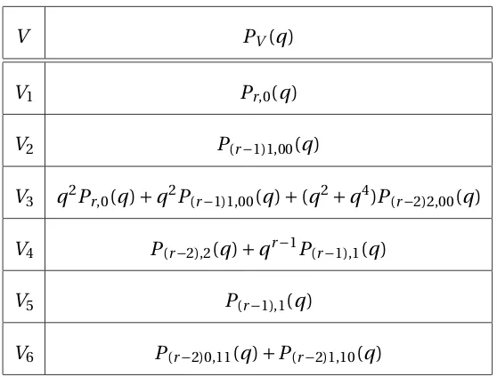
For r ≥3, the decomposition ofg⊗gis uniform. ∧2gdecomposes into a copy of g

and two dual representations with highest weights 2ω1+ωr−1 andω2+2ωr

respec-tively, while S2gdecomposes into the trivial representation, another copy ofg, and

two representations with highest weightsω2+ωr−1and 2ω1+2ωr respectively. In an

orthonormal basis forg, the corresponding elements of the family algebra are actually

symmetric or antisymmetric as matrices.

TheLkRlreduction relation gives us a relation∼on elements inV_ω₂₊_ωr−1; applying the

differential operatorD=

³

∂

xαc2

´

∂

∂x_α gives a relation equivalent to the multiples of the

(52)

the trivial representation,Dapplied to both sides of∼again gives a relation between

elements of theV_ω₂₊_ω_r₋₁representation; hence we get that the generalized exponents

ofV_ω₂₊_ω_r₋₁ plus a copy of {r, . . . , 2r} gives the generalized exponents ofV2ω1+2ωr.

Along with the fact thatV_ω1+ωr has generalized exponents 1, . . . ,r gives us enough

in-formation to get the full set of generalized exponents for the representations in

ques-tion, given in table 1. Note that the two copies ofV_ω₁₊_ω_r each give an independent set

of harmonic basis elements, one symmetric, one antisymmetric. We get that PV(q)

is equal to the Kostka polynomial forV, which are computable from Young Tableaux

[DLT94]. Hence we can easily check the results given.

Table 6.1: Generalized Exponents inC_ω₁₊_ω_r(Ar)

V PV(q)

V0 1

V_ω1+ωr q[r]q

V_ω₂₊_ω_r₋₁ q2 [r+1]_[2]q[r−2]q

q

V2ω1+2ωr q

2¡r₊₁

2

¢

q

V2ω1+ωr−1 q

3¡r

2

¢

q

V_ω₂₊2ωr q

3¡r

2

¢

(53)

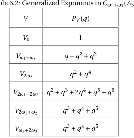
Table 6.2: Generalized Exponents inC_ω₁₊_ω₃(A3)

V PV(q)

V0 1

V_ω1+ωr q+q

2₊_q3

V2ω2 q

2₊_q4

V2ω1+2ω3 q

2₊_q3₊₂_q4₊_q5₊_q6

V2ω1+ω2 q

3₊_q4₊_q5

V_ω₂₊2ω3 q

(54)

Chapter 7 The

B

_r

,

C

_r

case

The cases ofBr andCr end up very similar, so we treat them both here. We start with

Cr since it is somewhat simpler. As with the previous chapter, we use the case ofr =3

as an example.

7.1 Diagrams

As in the Ar case, we can write the primitive Casimir operators as traces

ck=

ek+1

Because the invariant changes sign every time it passes an adjoint edge, we get that

the odd-degree traces vanish, matching the fact that Cr only has odd-degree

expo-nents and hence even degree primitive Casimir elements. ForCr, the exponents are

(55)

Similar to the Ar case, we have a Cayley-Hamilton identity on our matrices in the

ref-erence representation. Defining

dk=

X

2nimi=k

1

mi!

µ

−cni

2ni

¶mi

wheremini indicates a sum over distinctni, we get that

X

k

d₂r−kQk=0

where

Qk=

k

We call this the matrix Cayley-Hamilton identity, to distinguish it from the Casimir

Cayley-Hamilton identity

X

2

nimi=2r+2

1

mi!

µ

−cni

2ni

¶m_i

=0

which we get by multiplying the matrix Cayley-Hamilton identity byM2and then

tak-ing traces in the 2r-dimensional representation.

The adjoint projection for getting rid of internal adjoint edges is also different:

= 1₂ + 1₂

Note the directions of the symplectic forms; the first term on the right-hand side has

both symplectic forms attached to the top edge, where they cancel.

Now we wish to show that the tensor invariants in (T(Cr))Sp(r)are generated by tensor

(56)

All finite dimensional representations ofCr can be written in terms of the reference

representation, so we only have to worry about tensors with adjoint and reference

edges. The vertices are Clebsches between the adjoint andV⊗V∨, and the Levi-Civita

tensor onV.

Note that the reference representation, being of dimension 2r, has a Levi-Civita tensor

with 2rvectors coming out of it. Moreover, takingrcopies of the symplectic form and

antisymmetrizing all of the edges yields a multiple of the Levi-Civita tensor. Hence the

Levi-Civita tensor can be replaced by the symplectic form. Thus we only have loops

of the reference edges with adjoint edges attached, i.e. traces over the reference

repre-sentation.

7.2 Generators

The main result about the generators forCr is that there are again three of them:

Theorem 7.2.1(Generators). The family algebra for the adjoint representation of Cr is

generated by

M=

I O

R2=2

I O

S=

I O

Family Algebras and the Isotypic Components of g tensor g

University of Pennsylvania

ScholarlyCommons

Publicly Accessible Penn Dissertations

1-1-2014

Family Algebras and the Isotypic Components of g

tensor g

Matthew Tai

Follow this and additional works at:

http://repository.upenn.edu/edissertations

Part of the

Mathematics Commons

Recommended Citation

Family Algebras and the Isotypic Components of g tensor g

FAMILY ALGEBRAS AND THE ISOTYPIC COMPONENTS OF

g

⊗

g

Matthew Tai

Presented to the Faculties of the University of Pennsylvania

in

Partial Fulfillment of the Requirements for the

Degree of Doctor of Philosophy

2014

Supervisor of Dissertation

Alexandre Kirillov

Professor of Mathematics

Graduate Group Chairperson

David Harbater

Professor of Mathematics

Acknowledgments

Contents

List of Tables

Chapter 1

Introduction

1.1 Simple Lie Algebras and Exponents

1.2 Casimir Invariants

1.3 Generalized Exponents

Chapter 2

Introduction to Family Algebras

2.1 Definition of Family Algebras

2.2 Relation to the Generalized Exponents

2.3 Restriction to the Cartan subalgebra

Chapter 3

Results for

V

=

g

3.1 Algebraic Structure

3.2 Fake Degrees

Chapter 4

Diagrams

4.1 Casimir Operators and Structure Constants

4.2 Projections

4.3 Symmetrization

Chapter 5

Invariant Tensors

5.1 General Statement for most Classical Lie Algebras

5.2

A

5.3

B

5.4

C

5.5 Other simple Lie algebras

Chapter 6

The

A

r

case

6.1 Diagrams for

A

6.2 Structure of the Family Algebra

6.3 Sufficiency of the Generators

6.4 Proof of the Relations

6.5 The Sufficiency of the Relations

6.6 Generalized Exponents

Chapter 7

The

B

_⊗

₌

_r

_r

_r