Stable feature selection and classification algorithms for multiclass microarray data

(1)

R E S E A R C H

Open Access

Stable feature selection and classiﬁcation

algorithms for multiclass microarray data

Sebastian Student

*

and Krzysztof Fujarewicz

Abstract

Background: Recent studies suggest that gene expression profiles are a promising alternative for clinical cancer classification. One major problem in applying DNA microarrays for classification is the dimension of obtained data sets. In this paper we propose a multiclass gene selection method based on Partial Least Squares (PLS) for selecting genes for classification. The new idea is to solve multiclass selection problem with the PLS method and

decomposition to a set of two-class sub-problems: one versus rest (OvR) and one versus one (OvO). We use OvR and OvO two-class decomposition for other recently published gene selection method. Ranked gene lists are highly unstable in the sense that a small change of the data set often leads to big changes in the obtained ordered lists. In this paper, we take a look at the assessment of stability of the proposed methods. We use the linear support vector machines (SVM) technique in diﬀerent variants: one versus one, one versus rest, multiclass SVM (MSVM) and the linear discriminant analysis (LDA) as a classiﬁer. We use balanced bootstrap to estimate the prediction error and to test the variability of the obtained ordered lists.

Results: This paper focuses on effective identification of informative genes. As a result, a new strategy to find a small subset of significant genes is designed. Our results on real multiclass cancer data show that our method has a very high accuracy rate for different combinations of classification methods, giving concurrently very stable feature rankings.

Conclusions: This paper shows that the proposed strategies can improve the performance of selected gene sets substantially. OvR and OvO techniques applied to existing gene selection methods improve results as well. The presented method allows to obtain a more reliable classiﬁer with less classiﬁer error. In the same time the method generates more stable ordered feature lists in comparison with existing methods.

Reviewers: This article was reviewed by Prof Marek Kimmel, Dr Hans Binder (nominated by Dr Tomasz Lipniacki) and Dr Yuriy Gusev

Background

Recent studies suggest that gene expression profiles may represent a promising alternative for clinical cancer clas-sification. Molecular-based approaches have opened the possibility of investigating the activity of thousands of genes simultaneously and can be used to find genes involved in neoplasia. A well known problem in apply-ing microarrays in classification problem is dimension of obtained datasets. In work [1] authors listed three main sources of the instability of feature selection in biomarker discovery: choosing selection algorithms with-out considering stability, the existence of multiple sets of

*Correspondence: [email protected]

Institute of Automatic Control, Silesian University of Technology, Akademicka 16, 44-100 Gliwice, Poland

true markers and small number of samples. They sug-gested that the problem of small number of samples in high dimensional feature space is the most difficult one in biomarker discovery. Other authors indicate a tech-nical problems, like post-hybridization washing [2], or chip-specific systematic variations on the raw intensity level [3], which can cause errors in computed expres-sion levels and may have a big influence on the insta-bility of feature selection. In [4] authors denoted the same problems not only for microarray data, but also for proteomic mass spectometry data. Traditional statis-tical methodology for classification does not work well when there are more variables than samples. Thus, meth-ods able to cope with the high dimensionality of the data are needed. In this paper we focus on multiclass feature selection and classification problem, which are

(2)

intrinsically more difficult than their binary counterparts [5]. Gene selection for a classifier is a very important problem. Over the past few years many algorithms were proposed to solve this problem. However, most of the studies are designed for dimension reduction in two-class problems and only a few of them involve multitwo-class cases. In [6,7] authors underline, that selection of infor-mative features for a classifier is a crucial and delicate task. The optimal selection of informative genes for mul-ticlass analysis is still an open problem. We propose a gene selection method based on Partial Least Squares (PLS) [8,9]. Then we compare the results with the multi-class gene selection method proposed in [10], Recursive Feature Elimination (RFE) method [7] and the classical t-statistics.

The standard way to use the PLS algorithm is for feature extraction only and not for selecting signiﬁ-cant features. Here, we use this method for gene rank-ing. In [8] it has been shown how to use the PLS method for multiclass feature extraction. Also in [11] the author considers a PLS-based method to gene selec-tion, but for 2-class data only. The new idea is to use the PLS for multiclass feature selection. A well known method of solving the multiclass feature selec-tion problem is to take into consideraselec-tion ‘all classes at once’.

We propose a new method based on decomposition of a multiclass feature selection problem into a set of two-class problems that are used in one versus rest (OvR) and one versus one (OvO) techniques.

An important aspect of feature selection methods is the stability of obtained ordered lists [1,12]. In [1] we can ﬁnd a review that summarizes some stable feature selection methods and a big range of stability measures. Authors have noted that stable feature selection is a very important problem, and they have suggested to pay more attention on it.

In literature [13] most of the feature selection and classification methods are compared based on the accu-racy rate only. In general we can define the accuaccu-racy rate, as the percentage of correctly classified probes among all probes (in most cases in the validation set). It is very difficult to evaluate the methods only by the small differences in accuracy rate. In this paper we use the stability criterion and accuracy rate to clearly compare different gene ranking methods. By bet-ter stability, we mean less variability of the ranked lists obtained with the same method, but with slightly mod-ified datasets. The stability problem of gene lists is very important for their validation by biological methods and for the clinical applicability of molecular markers. For example, for long gene lists, experimentalists will test only the most important genes, in this case the top-ranked genes.

Methods

Symbols and abbreviations

l — number of samples; m — number of genes; g —

number of selected genes; L— list of selected genes;K

— number of classes; B — number of bootstrap

sam-ples; PLS — Partial least squares regression method; s — number of PLS components;w— PLS weight vector; SIMPLS, NIPALS — names of two used PLS algorithms; PLS+MCLASS — PLS based multiclass gene selection method with ‘all classes at once’ approach; PLS+OvO — PLS based multiclass gene selection method with ‘one versus one’ decomposition; PLS+OvR — PLS based multiclass gene selection method with ‘one versus rest’ decomposition; GS — gene selection method proposed in [10]; RFE — Recursive Feature Elimination gene selec-tion method; s1, s2 — stability score indicators; SVM OvO, SVM OvR, MSVM — support vector machines based classiﬁcation methods; LDA — linear discriminant analysis classiﬁcation method;

Bootstrap resampling

We use bootstrap technique [14] which has good perfor-mance for relatively small sample classification problems [15]. In literature we can find many publication using bootstrap resampling for genomic data [16-21]. Of course, the best way to test classification and gene selection meth-ods is to use an independent dataset. However, without such a dataset, the resampling approach is one of the best choice. For example in [16] we can see that resam-pling technique is useful for microarray data analysis, and the results can be validated by qPCR analysis with an extra and independent set of samples not used in the main analysis. In our opinion the main problem in case of microarray results validation is to find proper gene selection method for analyzed data.

Let us consider a dataset of size l, where X =

(x1,x2,. . .,xl)is the input matrix andY =(y1,y2,. . .,yl)

(3)

by constructing a set withBcopies of alll observations and then permuting the obtained set. Every l-element successive subset is one bootstrap sample.

The bootstrap resampling is computationally costly. We implemented it on a computer cluster using the MatlabMPI toolbox for parallel computation. The most important parameter for the bootstrap resampling tech-nique is the number of resampling iterationsB. We must find the compromise between analysis time and accuracy of predicted parameters. In our cases we use 500 resam-pling iterations of all stages of the classifier construction (i.e. gene preselection, gene selection and classifier learn-ing). We did not observed significant changes in the results for all used datasets, after increasing the number of iterations. Of course, the necessary iterations number can change after changing the dataset and depends especially on the number of probes. We generated 500 bootstrap samples only once to reduce the variability of results for all tested methods. The distribution of the misclassifica-tion rate obtained during all bootstrap runs was used to estimate the 95% confidence interval. The accuracy of the classifier and the confidence interval were calculated for subsets of first genes on the lists up to 30 genes.

Prediction error estimation

To estimate the prediction error (accuracy) we used the .632+ estimator [24]. The .632+ estimator described by Efron provides protection of overﬁtting, especially impor-tant for methods like SVM, where the resubstitution error is very small. In extreme case, when the resubstitution error is very small, and much smaller than the test error, the .632 [25] estimator provides too optimistic estimates for the true error. In this situation the .632+ estimator takes more weight to the test error part, than the .632 esti-mator. The detailed description for the .632+ estimator is given in the Appendix.

PLS-based feature selection method

In this section we propose a new method for selecting the most significant genes. It is based on partial least squares regression (PLSR) [26]. There are some other regres-sion methods like Lasso method [27] or ridge regresregres-sion [28]. It was shown that PLS method outperforms Lasso method in terms of identifying relevant predictors [29]. We also do not use the ridge regression, where it is a problem with estimation the ridge parameter. PLSR method is well known as a method for feature extrac-tion [8,30,31], but its applicaextrac-tion for selecting significant genes is less evident. PLS feature extraction method can be used for significance analysis of gene expression data [32,33]. The authors of [34] used jackknife of PLS compo-nents to interpret the importance of the variables (genes) for the PLS model. When we use the feature extraction techniques like those based on projection (e.g. principal

component analysis) or compression (e.g. based on infor-mation theory), we use all genes in our model (with different weights), and the accuracy of the classifier is esti-mated for all of the genes. In contrast to feature extraction, feature selection techniques do not alter the original rep-resentation of the variables, but only select their subset. Feature selection is very important for biomarker discov-ery, specifically for RT-PCR experiment and leads to new knowledge about the biology of the disease. In that case, the genes selected are more important than the classifier used. In Boulesteix [31,35], the PLS connection to other statistical methods is described. Boulesteix proved that in case of the data matrix scaled to unit variance and two-class two-classification the lists of genes obtained with ordered squared weight vectorw2from the first PLS component is of the same order as from F-statistics. It is equivalent to the t-test with equal variance and also with the BSS/WSS-statistics, where BSS denotes the between-group sum of squares and WSS the within-group sum of squares. In our comparison we did not scale the data to unit variance, but only centered the data. Boulesteix and Strimmer [35] describe and refer the connection of PLS to gene selection based on “variable importance in projection” (VIP) indica-tor proposed by Musumarra et al. [36], which indicates the importance of genes in the used PLS latent components. Musumarra et al. described the PLS method as dimension reduction method and used the weight vectors to order genes in term of their relevance for classification prob-lem. The main difference between our approach and VIP indicator is that in VIP method the latent components for classifier and the weight vector are used only for measure of the importance of each gene in PLS model.

In this paper we use the weight vector obtained from the PLS method to select the most important genes.

PLS aims at ﬁnding uncorrelated linear transformations of the original input features which have high covari-ance with the response features. Based on these latent components, PLS predicts response features (the task of regression) and reconstructs an original dataset matrix (the task of data modeling) at the same time. For dataset matrixXof sizel×mwithlprobes andmgenes we denote thel×1 vector of response valuey. The PLS components tii = 1,. . .,sare constructed to maximize the objective

criterion based on the sample covariance betweenyand linear combination of genes (PLS components)t = Xw. We search the weight vectorwsequentially, to satisfy the following criterion

wi=arg max

wT_w₌₁ cov

2_(Xw_,_y)_, ₍₁₎

subject to the orthogonality constraint

wT_i SXwj=0 1≤i<j

(4)

This criterion is the mostly used in literature as gen-eral description for PLS method. In case of multiclass categorical data this criterion can be simpliﬁed as men-tioned in [37] and maximize var(Xw) Cor2(Xw,Y). To derive components (named “latent variables” or scores), ti(i=1,. . .,s), the PLS decomposesXandyto produce a

bilinear representation of the data [38]

X=t1pT1 +t2p2T +. . .+tspTs +E (3)

y=t1q1+t2q2+. . .+tsqs+f,

where pi are loadings,qi are scalars and E,f are

resid-uals. The idea of PLS is to estimate loadings and scores by a regression. The PLS ﬁts a sequence of bilinear mod-els by least squares. At every stepi(i = 1,. . .,s) vector wi is estimated to obtain the PLS component that has

maximal sample covariance with the response variabley. Each componenttiis uncorrelated with all previously

con-structed components. There are two main PLS algorithms described in literature: NIPALS algorithm [39] and SIM-PLS algorithm [40]. The SIMSIM-PLS algorithm, is diﬀerent from NIPALS in two important ways: ﬁrst, successiveti

components are calculated explicitly as linear combina-tions of X and second, X is not deflated in each iteration. The SIMPLS algorithm will be assessed in accordance with the criteria eq. (1). In NIPALS the first PLS compo-nentt1is obtained on the basis of the covariance between X andy, and is qual to the first component of SIMPLS algorithm. Componentti(i=2,. . .,s), is computed using

the residuals of X and y from the previous step, which account for the variations left by the previous compo-nents. Maximal number of componentssis equal to the rank ofX.

As we say before the weight vector from SIMPLS algo-rithm sometimes referred toris applied to the originalX matrix and De Jong [40] showed that we can calculate the weightsrdirectly from the NIPALS algorithm

ri=wi(piwi)(−1), (4)

wherep_iare the loading andwiare the weight vector for

i-th component of NIPALS algorithm.

De Jong proved in [40] that for univariate response the score vectors ti(i = i,. . .,s) for NIPALS and SIMPLS algorithms are the same. In contrast to score vectors, the weight vectorswiandrifor NIPALS and SIMPLS respec-tively are different for i > 1. This phenomenon is a consequence of different method to compute the weights vectors. The wi vectors in NIPALS procedure are cal-culated with deflated data matrices Xi and Yi in each iteration, and the weights ri are obtained without the deflation step in SIMPLS algorithm. For this reason in this paper, we use the weight vectorswandrfrom both

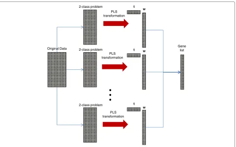
algorithms to determine the ranked list. In our method the sum of the w2_i over thes PLS components presents the gene importance vector and the “best genes” have the highest values in this vector. Firstggenes with the highest value in the gene importance vector are selected for the classifier. To test the optimal number of components we use the first squared weight vector and the sum of squared weight vectors from first 5 and 10 components. The stan-dard way to use PLS for a multiclass data, is to search for the best direction for maximization of the covariance between responses with all classes and linear combina-tion of genes. As we mencombina-tioned before, we compare our method based on decomposition of a multi-class feature selection problem into a set of two-class problems with a well known ‘all classes at once’ technique. For each two-class selections “best genes” are selected and one ranked gene list is constructed as follows: genes with the highest weight in all two-class selections are located at the top of the list, then genes with the second highest weights, and so on. We must underline, thatyfor two-class selections is coded as a vector with value 1 for the first class and−1 for the second class. For the ‘all classes at once’ technique yis a matrix withNrows and the number of columns is equal to the number of classes. In each row a class label has a value of 1 and−1. For our needs we introduce the notation PLS+MCLASS for ‘all classes at once’ technique and similarly PLS+OvO, PLS+OvR for two-class decom-position of the multiclass feature selection problem. On the Figure 1 we show the principals and essentials of the introduced method.

Stability analysis for ordered gene lists

In [6,41] authors have used resampling technique for test-ing the significance of the obtained results of microarray analysis. They have examined the influence of sample class label permutations and selection of exact number of randomly selected features on the classification accuracy. We can find in literature various applications of boot-strap technique for example to assess the stability of the cell lines cluster dendrogram in unsupervised microar-ray analysis [42]. In our article we use bootstrap resam-pling to examine the stability of obtained gene lists. By stability of an obtained gene list we understand similar-ity between lists from the same experiment, but with a slightly changed data set. To show the distance between different gene selection methods we use a method based on bootstrap resampling. This approach is based on the comparison of sets consisting of a fixed number of the topggenes. In this framework we consider the listLwith firstgtop-genes obtained from the entire dataset and lists Lb;b = 1, 2,. . .,Bobtained from everybofBbootstrap

iterations.

(5)

Original Data

2-class problem

PLS transformation

w

w t

t

Gene list

Figure 1PLS based gene selection method with two-class decomposition technique.

used Percentage of Overlapping Genes (POG) criterion [43] and modiﬁed POG indicator. The POG criterion takes into account only the content of gene lists, and ignores the gene order. The modiﬁed POG indicator does not ignore the gene order on compared lists. Both indica-tors are detailed described in the Appendix.

The second one is to visualize how obtained gene lists are stable by looking at descriptive plots. In the next section we introduce the detailed description of the stabil-ity plots used in this article.

Stability plots

To visualize the stability of the ordered gene lists we plot the boxplots of rank for each gene in the listL against ranks in allbbootstrap iteration listsLb;b = 1, 2,. . .,B.

We set the limit to determine which points are extreme to the rank out of the g gene list. Another way to visu-alize gene lists stability is to plot a so-called Bootstrap Based Feature Ranking (BBFR) plot [44]. The BBFR score, in opposite to indices s1 ands2, is calculated separately for each gene. The BBFR score for the gene numberjis deﬁned as

Qj=

B

b=1rbj

Bg , (5)

where rbj is the rank of the j-th gene in b-th bootstrap

iteration

rbj=g−ubj+1 (6)

for the top-scored generbj=g.

The maximum possible value of the Qj score is 1. It

means that one gene was top-ranked in allB bootstrap iterations. The scoreQjtakes into account the rankrbjof j-th gene in allBbootstrap iterations.

The modiﬁed BBFR scoreQ_jtakes into account only the presence of the genejin the listsLb;b=1, 2,. . .,B

Q_j=

B

b=1I(ubj≤g)

B . (7)

The maximum possible value of theQ_j score is 1. The 0 value indicates genes not included on the gene lists in all bootstrap iterations.

Both Qj and Q_j indices are sorted and plotted in

(6)

Datasets

In our study we chose three publicly available multiclass microarray datasets. The ﬁrst is the LUNG dataset pub-lished by [45]. It consists of 254 samples of 4 subtypes of lung carcinomas and normal samples. Samples were normalized by RMA and GA annotation [46]. Each sam-ple has 8359 gene expression levels after re-annotation. The data is available at http://www.broadinstitute.org/ mpr/lung/. The second is the MLL dataset published by [47]. It consists of 72 samples of 3 subtypes of leukemia cancer classes. Samples was normalized by RMA and GA annotation [46]. Each sample has 8359 gene expression levels after re-annotation. The data is available at http://www.broadinstitute.org/cgi-bin/ cancer/publications/pub paper.cgi?mode=view&paper id =63. The third is the SRBCT dataset published by [48]. It consists of 83 samples of 4 subtypes of small, round blue cell tumors. Each sample has 2308 gene expression levels. The data is available at http://www.biomedcentral. com/content/supplementary/1471-2105-7-228-s4.tgz [10]. The results for the LUNG dataset are presented in the main body of this paper, and the results for MLL and SRCT datasets are presented in the Appendix section.

Results and Discussion

We chose three multiclass microarray datasets (detailed described in the Datasets section) for our experiments.

For the numerical experiment we use SVM method clas-siﬁcation method in three variants OvO, OvR, MSVM

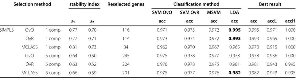
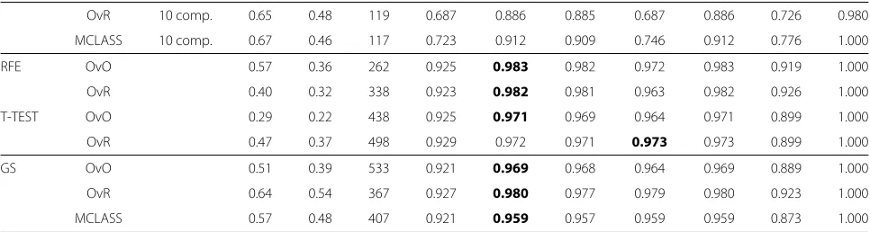
and LDA method. These methods are common used in microarray classification problems [49-51]. We demon-strate the usefulness of the proposed methodology to select significant genes with decomposition technique and the PLS method. All methods: PLS+OvO, PLS+OvR and PLS+MCLASS were tested and compared with other methods. As it has been mentioned before, we executed 500 bootstrap iterations for each method. Because the most important task is to find a small number of infor-mative genes, we classify this data in every bootstrap iteration for diverse number of best genes up to 30 genes. In Tables 1, 2 and 3 (Tables are available in the Appendix) we collect all results for all tested methods. For all plots we use the classifier with the best clas-sification rate chosen separately for all tested method. The PLS algorithm and the number of PLS components were chosen with respect to the best accuracy rate crite-rion. In most cases thervector calculated from SIMPLS method was better than the vector w calculated from NIPALS algorithm for more than one component. Only for PLS+MCLASS method the accuracy rate is higher when we use more than 1 PLS component. In our study we also applied a method searching for the optimal num-ber of components based on leave one out classification error on training samples and the SVM classifier (results not showed here). In general the results for classification accuracy rate were not significantly better and in some cases even worse. In all tables we bolded the best accu-racy rate for tested classification methods and variants of PLS method (algorithm and number of PLS components).

0.9 0.95 1

0 0.2 0.4 0.6 0.8 1

accuracy

stabilit

y

inde

x

PLS +O

vR

PLS+OvO GS+MCLASS

GS +Ov

R

PLS +MC

LASS GS+O

vO

T-T

est+OvR _RFE+Ov O

RFE+OvR T-T

est +Ov

O

(7)

0 5 10 15 20 25 30 0.5

0.55 0.6 0.65 0.7 0.75 0.8 0.85 0.9 0.95 1

Number of genes

PLS+OvO PLS+OvR PLS+MCLASS GS+OvO GS+OvR GS+MCLASS RFE+OvO RFE+OvR T-TEST+OvO T-TEST+OvR

Figure 3Accuracy of classiﬁcation obtained by successive gene set reduction selected with all feature selection methods of the best classiﬁer for LUNG data.

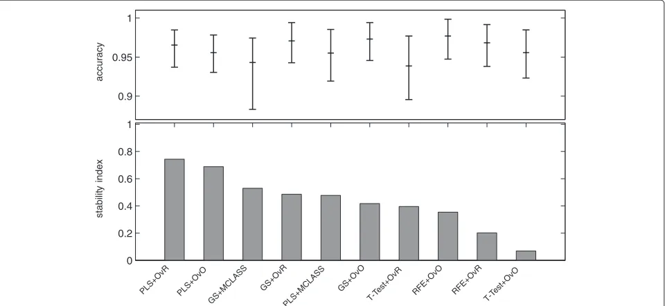
In the last columns we show the standard deviations val-ues for the best classiﬁer. The comparison of accuracy rate and stability indexs2 for all tested datasets proves the advantage of the PLS method (Figure 2). In all cases stability indexs2for the PLS method with decomposition technique is higher than the score for the PLS+MCLASS method. Only for the LUNG dataset the stability index for decomposition version of the GS method is lower than with the GS+MCLASS method (Figure 2). However, in this case, the accuracy rate for the GS+MCLASS was

about 3% lower than for the GS+OvO method. Conse-quently, looking at all the classification accuracies and the 95% confidence interval as shown in Tables 1, 2 and 3, one general conclusion is that there are no signifi-cant differences between best gene selection methods. Typically, our methods outperform the other methods when we compare the stability index. Another conclusion is that more components spoil the stability of obtained genes lists and the classification error is not significantly smaller.

0 5 10 15 20 25 30 35 40 45 50

0 0.1 0.2 0.3 0.4 0.5 0.6 0.7 0.8 0.9 1

Numbers of genes

PLS+OvO PLS+OvR PLS+MCLASS GS+OvO GS+OvR GS+MCLASS RFE+OvO RFE+OvR T-Test+OvO T-Test+OvR Ideal curve

(8)

On Figure 3 we can see how many genes we need to obtain good prediction. For the arbitrary changed number of features selected we built the model and estimate the accuracy rate. We do not use the accuracy rate to estimate the number of selected genes as in backward elimina-tion features selecelimina-tion. When we compare the results for diﬀerent datasets (for example Figure 3, and Figure 8,

Figure 9 from Appendix), we can see, that in all cases the two class decomposition based gene selection meth-ods are better for different number of selected genes, when we consider the accuracy rate into account. How-ever, we can see that there are big differences between used methods, especially, when we use a very small num-ber of genes. We also observe, slight different accuracy

0 5 10 15 20 25 30

rank in the orginal dataset Gene ranking in the bootstrap data sets

PLS+OvO approach

1 2 3 4 5 6 7 8 9 10 11 12 13 14 15 16 17 18 19 20 21 22 23 24 25 26 27 28 29 30 0 5 10 15 20 25 30

PLS+OvR approach

1 2 3 4 5 6 7 8 9 10 11 12 13 14 15 16 17 18 19 20 21 22 23 24 25 26 27 28 29 30

0 5 10 15 20 25 30

rank in the orginal dataset

PLS+MCLASS approach

1 2 3 4 5 6 7 8 9 10 11 12 13 14 15 16 17 18 19 20 21 22 23 24 25 26 27 28 29 30 0 5 10 15 20 25 30

GS+MCLASS approach

1 2 3 4 5 6 7 8 9 10 11 12 13 14 15 16 17 18 19 20 21 22 23 24 25 26 27 28 29 30

0 5 10 15 20 25 30

GS+OvR approach

1 2 3 4 5 6 7 8 9 10 11 12 13 14 15 16 17 18 19 20 21 22 23 24 25 26 27 28 29 30

0 5 10 15 20 25 30

RFE+OvR approach

1 2 3 4 5 6 7 8 9 10 11 12 13 14 15 16 17 18 19 20 21 22 23 24 25 26 27 28 29 30

0 5 10 15 20 25 30

T−TEST+OvR approach

1 2 3 4 5 6 7 8 9 10 11 12 13 14 15 16 17 18 19 20 21 22 23 24 25 26 27 28 29 30 0

5 10 15 20 25 30

GS+OvO approach

1 2 3 4 5 6 7 8 9 10 11 12 13 14 15 16 17 18 19 20 21 22 23 24 25 26 27 28 29 30

0 5 10 15 20 25 30

RFE+OvO approach

1 2 3 4 5 6 7 8 9 10 11 12 13 14 15 16 17 18 19 20 21 22 23 24 25 26 27 28 29 30

0 5 10 15 20 25 30

T−TEST+OvO approach

1 2 3 4 5 6 7 8 9 10 11 12 13 14 15 16 17 18 19 20 21 22 23 24 25 26 27 28 29 30

(9)

results for the diﬀerent data sets and selected gene number, especially in the dynamics of accuracy rate for increased number of genes. This means, that the num-ber of selected genes depends on dataset used and is important for distinguish the best gene selection method (for example comparison of Accuracy rate results for LUNG data on Figure 3 and for MLL data set Figure 8 from Appendix).

In all tested datasets the 30 genes were suﬃcient enough to obtain a high accuracy rate. In all datasets the decomposition variants of the GS method outperform the GS+MCLASS method. The PLS+OvO and PLS+OvR methods perform at least comparably well and for the MLL dataset the accuracy rate was higher for diﬀerent number of selected genes.

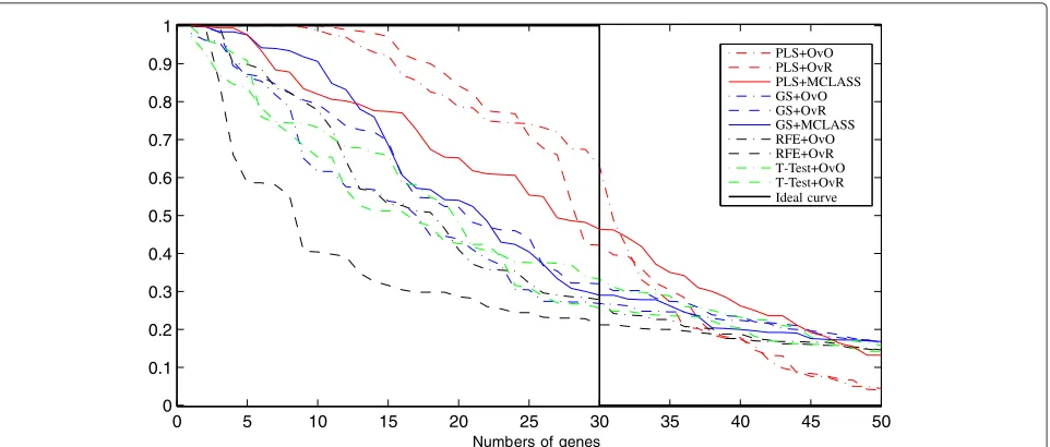
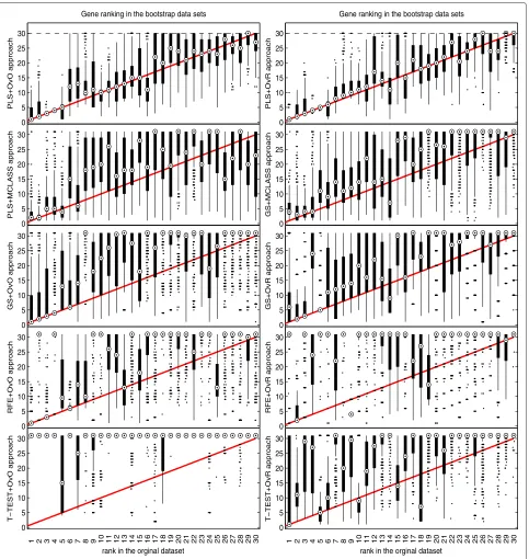
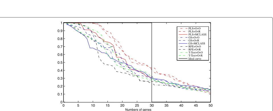
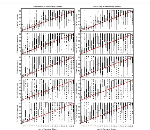
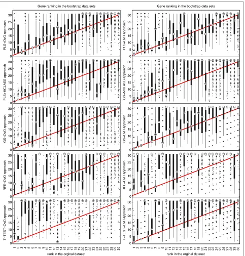
The bootstrap-based feature ranking (BBFR) is com-puted for a list of 30 genes. The BBFR ranking (Figure 4) and the boxplots of rank for each gene in the bootstrap lists versus the whole dataset gene list (Figure 5) confirm the advantage of the proposed gene selection method. For all datasets only the BBFR curves for PLS+OvO and PLS+OVR are very close to ideal curve. This means that the same genes are reselected frequently in most boot-strap iterations. In Tables 1, 2 and 3 we can see, that for the PLS method we observe the smallest number of all genes selected in all bootstrap iteration 30-genes lists (reselected genes column). That means, that the reproducibility of the PLS method is very high in con-trast to other methods, where we observe more than one hundred genes more. Our conclusion for different number of selected genes is confirmed by the boxplots in Figure 5 for tested methods. The figures illustrate how close the bootstrap based feature ranking is to the ranking obtained from the whole datasets for the first 30 genes. The red line indicate the ideal case. The best reproducibility is found with the PLS method. The worst reproducibility is found for the classical T-TEST and RFE method.

Conclusions

In this paper we proposed a new PLS-based method to select significant genes. Our results have shown that this gene selection method gives very good accuracy rate and stability of obtained gene lists. The principal of PLS is based on the maximization of the covariance criterion, which can lead to good generalization ability and stabil-ity. In our opinion this is a reason of the good results obtained with PLS method. Another important result is the fact that it is more effective to solve a multiclass feature selection by splitting it into a set of two-class problems and merging the results in one gene list. The explana-tion for these result can be the difference between used methods: the idea of MCLASS approach is to look for

genes able to distinguish between all classes simultane-ously. Such genes are more difficult to find, and they can have smaller discriminatory power. This problem do not exist in the decomposed multiclass problem for OvO and OvR approaches. From the methodological side we sup-pose, that the MCLASS multiclass feature selection meth-ods are not so good developed, as the 2-class methmeth-ods, and this fact can be the explanation for our results. The comparison to other feature selection methods shows that the gene lists stability index is the highest for PLS with OvR and OvO techniques. In two cases the stability index is slightly better for PLS+MCLASS method with one PLS component, but the accuracy rate for this method is sig-nificantly worse. All other methods indicated much worse stability of obtained gene lists. We can observe that using the GS method with 2-class decomposition technique improves the accuracy rate and with two of the datasets gene list stability increased as well. Another advantage of the 2-class decomposition technique for gene selection methods is easy interpretation of the results by biologists. In all cases the ‘all classes at once’ technique of PLS and GS methods achieves worse classification accuracy than their 2-class versions. The presented method makes it possi-ble to obtain more stapossi-ble gene selection lists and a more reliable classifier with less classifier error. We show that accuracy rate assessing accompanied with the gene sta-bility analysis gives more reliable evaluation of various gene selection methods. Of course our methods can be applicable also to other high dimensional data where we consider classification problems such as protein microar-rays, DNA copy number variation, exome profiling and RNAseq. In all cases, where the dataset has much more features than observations it is recommended to take into consideration the accuracy rate, but also the stability score.

Appendix Stability indices

In general there are two diﬀerent approaches to measure the stability of gene lists. The ﬁrst approach takes into account only the content of gene lists, and ignores the gene order. The second one does not ignore the gene order on compared lists.

One of the most frequently used criteria is the Per-centage of Overlapping Genes (POG) [43], belong-ing to ﬁrst class of stability measures. In the sim-plest case it measures the similarity between two lists L1 and L2 of the size g. Let k be the size of the intersection of L1 and L2. Then POG is deﬁned as

s1=k/g.

(10)

the listL. For the top-scored geneuj= 1. Similarly,ubjis

the placement of thej-th gene in the listLb. The POG is

calculated as

s1=

B

b=1

g

j=1I(uj≤g∧ubj≤g)

Bg , (8)

whereIdenotes the indicator function

I(A)=

1 ifA=true

0 ifA=false

(9)

We introduce the modiﬁed relatives2score to estimate the similarity between all lists

s2=1−

B

b=1 g

j=1

|uj−ubj|

Bg(g+1)/2. (10)

In opposite to previous indicators1, it does not ignore the rank of the selected genes within the considered subset, hence it belongs to the second mentioned class of stability measures. The value for the gene that is out ofLbis set to g+1. The value of functionss1ands2is scaled to the inter-val0, 1and the higher value indicates better stability of the obtained gene list.

Another indicator used to estimate the stability of an obtained gene list is given by the number of genes that were selected at least one time in all bootstrap samples. The best value is g and the worst is Max(G,Bg) where Gis the number of all genes. This approach is equal to the number of genes with a non-zero score in the Boot-strap Based Feature Ranking (BBFR) (described in the next section).

Prediction error estimation

To estimate the prediction error we use the .632+ estima-tor [24]. First we must deﬁne the prediction model asfˆ(X) which can be estimated from a training sample. The loss function for measuring errors betweenYandfˆ(X)we can describe asL(Y,fˆ(X)). This function returns 0 if response Y equals predicted valuefˆ(X)and 1 otherwise. Now we can deﬁne the resubstitution error

Errresub=

1 l

l

i=1 L

yi,fˆ(xi)

, (11)

where fˆ(xi) is the predicted value at xi of the whole

dataset. This predictor can make overﬁtted predictions and the estimated error rate will be downward biased. It demonstrates why we obtain error estimator for test data sets in the form

Errtest=

1 B

B

b=1 1

|Cb|

i∈|Cb|

Lyi,fˆ∗b(xi)

. (12)

The model trained on a training set will be tested on other samples and not used to ﬁt the model. This provides pro-tection against overﬁtting. As we have mentioned before, we compute the error rate forBsetsCbcontaining

sam-ples that do not appear inb-th bootstrap sample and|Cb| is a number of such samples. This estimator will overes-timate the true prediction error, and when the test set is small it can have high variance [15]. To resolve this prob-lem we use the .632+ estimator. This is a modified version of the .632 estimator to avoid downward bias in overfit-ting case of our classifier. Defineγ to be the error rate of our prediction rule if the inputs and class labels are inde-pendent. Letpˆk be the observed proportion of responses yiequalkand letqˆkbe the proportion of predictionsfˆ(xi)

equalk, wherekis the class label ofKclass. Then

ˆ

γ =

K

k=1 ˆ

pk

1− ˆqk . (13)

The relative overﬁtting rate is

ˆ

R= Errtest−Errresub ˆ

γ −Errresub

. (14)

Now we can deﬁne the .632+ estimator by

Err(.632+)=(1− ˆw)Errresub+ ˆwErrtest, (15)

ˆ

w= 0.632

1−0.368Rˆ. (16)

When there is no overﬁtting problem the .632+ estimator is equal to the .632 estimator

(11)

Tables

Table 1 The bootstrap based classification accuracies, stability index and number of reselected genes in all bootstrap samples of the SVM-classifier and the LDA-classifier based on all tested gene selection methods, on the LUNG dataset

method stability index Reselected genes Classiﬁcation method Best result

SVM OvO SVM OvR MSVM LDA

s1 s2 acc acc acc acc acc accL accH

SIMPLS OvO 1 comp. 0.86 0.69 84 0.954 0.946 0.951 0.956 0.956 0.930 0.978

OvR 1 comp. 0.86 0.74 78 0.950 0.945 0.947 0.965 0.965 0.937 0.985

MCLASS 1 comp. 0.88 0.79 70 0.917 0.882 0.892 0.895 0.917 0.868 0.956

OvO 5 comp. 0.60 0.51 186 0.950 0.928 0.944 0.966 0.966 0.933 0.986

OvR 5 comp. 0.71 0.61 170 0.958 0.946 0.953 0.963 0.963 0.940 0.986

MCLASS 5 comp. 0.75 0.58 103 0.953 0.945 0.949 0.917 0.953 0.920 0.979

OvO 10 comp. 0.58 0.44 214 0.949 0.928 0.941 0.946 0.949 0.913 0.979

OvR 10 comp. 0.63 0.49 228 0.955 0.944 0.950 0.961 0.961 0.931 0.983

MCLASS 10 comp. 0.72 0.48 128 0.955 0.949 0.950 0.943 0.955 0.919 0.985

NIPALS OvO 1 comp. 0.86 0.69 84 0.954 0.946 0.951 0.956 0.956 0.930 0.978

OvR 1 comp. 0.86 0.74 78 0.950 0.945 0.947 0.965 0.965 0.937 0.985

MCLASS 1 comp. 0.88 0.79 70 0.917 0.882 0.892 0.895 0.917 0.868 0.956

OvO 5 comp. 0.68 0.60 151 0.949 0.932 0.943 0.956 0.956 0.924 0.980

OvR 5 comp. 0.76 0.62 126 0.954 0.946 0.949 0.954 0.954 0.923 0.980

MCLASS 5 comp. 0.74 0.62 111 0.949 0.940 0.944 0.930 0.949 0.907 0.979

OvO 10 comp. 0.66 0.46 143 0.946 0.920 0.936 0.927 0.946 0.907 0.978

OvR 10 comp. 0.71 0.51 134 0.950 0.938 0.944 0.936 0.950 0.910 0.979

MCLASS 10 comp. 0.73 0.55 121 0.951 0.944 0.947 0.911 0.951 0.912 0.979

RFE OvO 0.44 0.35 487 0.962 0.953 0.961 0.977 0.977 0.947 0.999

OvR 0.30 0.20 808 0.965 0.961 0.964 0.968 0.968 0.938 0.992

T-TEST OvO 0.09 0.07 333 0.956 0.939 0.951 0.951 0.956 0.923 0.985

OvR 0.47 0.40 624 0.939 0.925 0.934 0.850 0.939 0.896 0.977

GS OvO 0.52 0.42 453 0.962 0.944 0.957 0.973 0.973 0.946 0.994

OvR 0.62 0.49 305 0.964 0.953 0.961 0.971 0.971 0.943 0.994

MCLASS 0.65 0.53 243 0.935 0.900 0.921 0.943 0.943 0.883 0.974

a_{The number of selected genes is set to 30 In last 3 columns is the best accuracy rate together with their bootstrap based standard deviations (accL,accH). The number} of reselected genes is the sum of non zero bootstrap-based feature ranked genes (BBFR).

Table 2 The bootstrap based classification accuracies, stability index and number of reselected genes in all bootstrap samples of the SVM-classifier and the LDA-classifier based on all tested gene selection methods, on the MLL dataset

Selection method stability index Reselected genes Classiﬁcation method Best result

SIMPLS OvO 1 comp. 0.77 0.70 116 0.971 0.973 0.972 0.995 0.995 0.971 1.000 OvR 1 comp. 0.77 0.71 114 0.973 0.974 0.972 0.993 0.993 0.969 1.000 MCLASS 1 comp. 0.81 0.73 84 0.962 0.970 0.967 0.965 0.970 0.915 1.000

OvO 5 comp. 0.64 0.50 245 0.975 0.978 0.977 0.978 0.978 0.936 1.000

OvR 5 comp. 0.63 0.52 224 0.976 0.978 0.975 0.981 0.981 0.943 0.995

(12)

Table 2 The bootstrap based classification accuracies, stability index and number of reselected genes in all bootstrap samples of the SVM-classifier and the LDA-classifier based on all tested gene selection methods, on the MLL dataset continued

OvR 10 comp. 0.52 0.40 281 0.974 0.975 0.973 0.971 0.975 0.936 1.000

MCLASS 10 comp. 0.58 0.47 236 0.975 0.976 0.974 0.972 0.976 0.936 1.000

NIPALS OvO 1 comp. 0.77 0.70 116 0.971 0.973 0.972 0.995 0.995 0.971 1.000

OvR 1 comp. 0.77 0.71 114 0.973 0.974 0.972 0.993 0.993 0.969 1.000

MCLASS 1 comp. 0.81 0.73 84 0.962 0.970 0.967 0.965 0.970 0.915 1.000

OvO 5 comp. 0.62 0.50 221 0.974 0.975 0.974 0.975 0.975 0.924 0.995

OvR 5 comp. 0.62 0.53 198 0.975 0.976 0.975 0.977 0.977 0.938 0.995

MCLASS 5 comp. 0.67 0.53 188 0.974 0.976 0.974 0.979 0.979 0.943 0.995

OvO 10 comp. 0.62 0.46 211 0.973 0.975 0.974 0.963 0.975 0.928 1.000

OvR 10 comp. 0.61 0.47 196 0.970 0.971 0.970 0.960 0.971 0.971 1.000

MCLASS 10 comp. 0.63 0.51 204 0.971 0.973 0.971 0.957 0.973 0.973 1.000

RFE OvO 0.58 0.48 318 0.975 0.977 0.974 0.982 0.982 0.940 0.995

OvR 0.47 0.36 401 0.976 0.977 0.975 0.988 0.988 0.947 1.000

T-TEST OvO 0.55 0.42 448 0.972 0.978 0.976 0.987 0.987 0.945 1.000

OvR 0.59 0.49 534 0.977 0.978 0.977 0.981 0.981 0.935 0.995

GS OvO 0.62 0.54 489 0.971 0.977 0.975 0.982 0.982 0.943 0.995

OvR 0.64 0.50 490 0.977 0.977 0.976 0.986 0.986 0.947 0.995

MCLASS 0.59 0.43 526 0.963 0.967 0.965 0.970 0.970 0.915 0.995

OvO 10 comp. 0.56 0.33 268 0.969 0.972 0.971 0.960 0.972 0.919 1.000

a_{The number of selected genes is set to 30. In last 3 columns is the best accuracy rate together with their bootstrap based standard deviations (accL,accH). The} number of reselected genes is the sum of non zero bootstrap-based feature ranked genes (BBFR).

Table 3 The bootstrap based classification accuracies, stability index and number of reselected genes in all bootstrap samples of the SVM-classifier and the LDA-classifier based on all tested gene selection methods, on the SRBCT dataset

Selection method stability index Reselected genes Classiﬁcation method Best result

SIMPLS OvO 1 comp. 0.71 0.60 127 0.867 0.977 0.976 0.941 0.977 0.913 1.000 OvR 1 comp. 0.74 0.59 137 0.882 0.980 0.980 0.952 0.980 0.912 1.000 MCLASS 1 comp. 0.58 0.39 240 0.807 0.930 0.932 0.829 0.932 0.797 1.000

OvO 5 comp. 0.52 0.36 204 0.831 0.970 0.968 0.929 0.970 0.896 1.000

OvR 5 comp. 0.63 0.43 173 0.867 0.981 0.979 0.964 0.981 0.926 1.000

MCLASS 5 comp. 0.72 0.58 133 0.856 0.979 0.978 0.945 0.979 0.903 1.000 OvO 10 comp. 0.40 0.25 239 0.817 0.961 0.958 0.910 0.961 0.873 1.000

OvR 10 comp. 0.45 0.23 237 0.839 0.977 0.974 0.942 0.977 0.912 1.000

MCLASS 10 comp. 0.63 0.41 133 0.832 0.975 0.973 0.931 0.975 0.912 1.000

NIPALS OvO 1 comp. 0.71 0.60 127 0.867 0.977 0.976 0.941 0.977 0.913 1.000

OvR 1 comp. 0.74 0.59 137 0.882 0.980 0.980 0.952 0.980 0.912 1.000

MCLASS 1 comp. 0.58 0.39 240 0.807 0.930 0.932 0.829 0.932 0.797 1.000

OvO 5 comp. 0.65 0.45 152 0.726 0.920 0.914 0.775 0.920 0.785 1.000

OvR 5 comp. 0.68 0.47 129 0.748 0.935 0.932 0.787 0.935 0.819 1.000

MCLASS 5 comp. 0.69 0.48 133 0.805 0.965 0.962 0.861 0.965 0.873 1.000

(13)

Table 3 The bootstrap based classification accuracies, stability index and number of reselected genes in all bootstrap samples of the SVM-classifier and the LDA-classifier based on all tested gene selection methods, on the SRBCT dataset Continued

OvR 10 comp. 0.65 0.48 119 0.687 0.886 0.885 0.687 0.886 0.726 0.980

MCLASS 10 comp. 0.67 0.46 117 0.723 0.912 0.909 0.746 0.912 0.776 1.000

RFE OvO 0.57 0.36 262 0.925 0.983 0.982 0.972 0.983 0.919 1.000

OvR 0.40 0.32 338 0.923 0.982 0.981 0.963 0.982 0.926 1.000

T-TEST OvO 0.29 0.22 438 0.925 0.971 0.969 0.964 0.971 0.899 1.000

OvR 0.47 0.37 498 0.929 0.972 0.971 0.973 0.973 0.899 1.000

GS OvO 0.51 0.39 533 0.921 0.969 0.968 0.964 0.969 0.889 1.000

OvR 0.64 0.54 367 0.927 0.980 0.977 0.979 0.980 0.923 1.000

MCLASS 0.57 0.48 407 0.921 0.959 0.957 0.959 0.959 0.873 1.000

a_{The number of selected genes is set to 30. In last 3 columns is the best accuracy rate together with their bootstrap based standard deviations (accL,accH). The} number of reselected genes is the sum of non zero bootstrap-based feature ranked genes (BBFR)

Figures for MLL and SEBCT data

0.9 0.95 1

0 0.2 0.4 0.6 0.8 1

accuracy

stabilit

y

inde

x

PLS+OvR PLS+OvO PLS+MCLAS

S

GS+OvO GS+OvR T-T

est+OvR RFE+Ov O

GS+MC LASS

T-Test +OvO

RFE+OvR

Figure 6Stability indexs2(bar chart) and accuracy of classification (dot chart) with the 95% confidence interval of the best classifier on the tested feature selection methods for MLL data.

0.9 0.95 1

0 0.2 0.4 0.6 0.8 1

accuracy

st

ab

ilit

y

in

d

ex

PLS+OvO PLS+OvR PLS+MCLASS

GS+OvR GS

+MC LASS

GS+OvO T-Tes

t+Ov R

RFE+Ov O

RFE+OvR T-T

est+Ov O

Figure 7Stability indexs2(bar chart) and accuracy of classification (dot chart) with the 95% confidence interval of the best classifier on

(14)

0 5 10 15 20 25 30 0.75

0.8 0.85 0.9 0.95 1

Number of genes

Figure 8Accuracy of classiﬁcation obtained by successive gene set reduction selected with all feature selection methods of the best classiﬁer for MLL data.

0 5 10 15 20 25 30

0.4 0.5 0.6 0.7 0.8 0.9 1

Number of genes

Figure 9Accuracy of classiﬁcation obtained by successive gene set reduction selected with all feature selection methods of the best classiﬁer for SRBCT data.

0 5 10 15 20 25 30 35 40 45 50

0 0.1 0.2 0.3 0.4 0.5 0.6 0.7 0.8 0.9 1

Numbers of genes

(15)

0 5 10 15 20 25 30 35 40 45 50 0

0.1 0.2 0.3 0.4 0.5 0.6 0.7 0.8 0.9 1

Numbers of genes

Figure 11Results of bootstrap-based feature ranking (BBFR) for the ﬁrst 50 genes for SRBCT data.In the ideal case (when gene lists are perfectly reproducible) the BBFR score reaches a value of 1 for the ﬁrst selected genes and 0 for the rest (black curve).

0 5 10 15 20 25 30

PLS+OvO approach

1 2 3 4 5 6 7 8 9 10 11 12 13 14 15 16 17 18 19 20 21 22 23 24 25 26 27 28 29 30 0 5 10 15 20 25 30

PLS+OvR approach

1 2 3 4 5 6 7 8 9 10 11 12 13 14 15 16 17 18 19 20 21 22 23 24 25 26 27 28 29 30

0 5 10 15 20 25 30

PLS+MCLASS approach

1 2 3 4 5 6 7 8 9 10 11 12 13 14 15 16 17 18 19 20 21 22 23 24 25 26 27 28 29 30 0 5 10 15 20 25 30

GS+MCLASS approach

1 2 3 4 5 6 7 8 9 10 11 12 13 14 15 16 17 18 19 20 21 22 23 24 25 26 27 28 29 30

0 5 10 15 20 25 30

GS+OvR approach

1 2 3 4 5 6 7 8 9 10 11 12 13 14 15 16 17 18 19 20 21 22 23 24 25 26 27 28 29 30

0 5 10 15 20 25 30

RFE+OvR approach

1 2 3 4 5 6 7 8 9 10 11 12 13 14 15 16 17 18 19 20 21 22 23 24 25 26 27 28 29 30

0 5 10 15 20 25 30

1 2 3 4 5 6 7 8 9 ₁₀ ₁₁ ₁₂ ₁₃ ₁₄ ₁₅ ₁₆ ₁₇ ₁₈ ₁₉ ₂₀ ₂₁ ₂₂ ₂₃ ₂₄ ₂₅ ₂₆ ₂₇ ₂₈ ₂₉ ₃₀ 0

5 10 15 20 25 30

GS+OvO approach

1 2 3 4 5 6 7 8 9 10 11 12 13 14 15 16 17 18 19 20 21 22 23 24 25 26 27 28 29 30

0 5 10 15 20 25 30

RFE+OvO approach

1 2 3 4 5 6 7 8 9 10 11 12 13 14 15 16 17 18 19 20 21 22 23 24 25 26 27 28 29 30

0 5 10 15 20 25 30

1 2 3 4 5 6 7 8 9 ₁₀ ₁₁ ₁₂ ₁₃ ₁₄ ₁₅ ₁₆ ₁₇ ₁₈ ₁₉ ₂₀ ₂₁ ₂₂ ₂₃ ₂₄ ₂₅ ₂₆ ₂₇ ₂₈ ₂₉ ₃₀

(16)

0 5 10 15 20 25 30

PLS+OvO approach

1 2 3 4 5 6 7 8 9 10 11 12 13 14 15 16 17 18 19 20 21 22 23 24 25 26 27 28 29 30 0 5 10 15 20 25 30

PLS+OvR approach

1 2 3 4 5 6 7 8 9 10 11 12 13 14 15 16 17 18 19 20 21 22 23 24 25 26 27 28 29 30

0 5 10 15 20 25 30

PLS+MCLASS approach

1 2 3 4 5 6 7 8 9 10 11 12 13 14 15 16 17 18 19 20 21 22 23 24 25 26 27 28 29 30 0 5 10 15 20 25 30

GS+MCLASS approach

1 2 3 4 5 6 7 8 9 10 11 12 13 14 15 16 17 18 19 20 21 22 23 24 25 26 27 28 29 30

0 5 10 15 20 25 30

GS+OvR approach

1 2 3 4 5 6 7 8 9 10 11 12 13 14 15 16 17 18 19 20 21 22 23 24 25 26 27 28 29 30

0 5 10 15 20 25 30

RFE+OvR approach

1 2 3 4 5 6 7 8 9 10 11 12 13 14 15 16 17 18 19 20 21 22 23 24 25 26 27 28 29 30

0 5 10 15 20 25 30

1 2 3 4 5 6 7 8 9 ₁₀ ₁₁ ₁₂ ₁₃ ₁₄ ₁₅ ₁₆ ₁₇ ₁₈ ₁₉ ₂₀ ₂₁ ₂₂ ₂₃ ₂₄ ₂₅ ₂₆ ₂₇ ₂₈ ₂₉ ₃₀ 0

5 10 15 20 25 30

GS+OvO approach

1 2 3 4 5 6 7 8 9 10 11 12 13 14 15 16 17 18 19 20 21 22 23 24 25 26 27 28 29 30

0 5 10 15 20 25 30

RFE+OvO approach

1 2 3 4 5 6 7 8 9 10 11 12 13 14 15 16 17 18 19 20 21 22 23 24 25 26 27 28 29 30

0 5 10 15 20 25 30

1 2 3 4 5 6 7 8 9 ₁₀ ₁₁ ₁₂ ₁₃ ₁₄ ₁₅ ₁₆ ₁₇ ₁₈ ₁₉ ₂₀ ₂₁ ₂₂ ₂₃ ₂₄ ₂₅ ₂₆ ₂₇ ₂₈ ₂₉ ₃₀

Figure 13Comparison of rank boxplots in the bootstrap samples against rank in the original data set on all tested methods for SRBCT data.

Reviewer’s report 1 Prof Marek Kimmel Report form:

As the authors state, “gene expression profiles are a promising alternative for clinical cancer classification”. The well-known difficulty is the large dimension of the vector of data, compared to the usually modest number of independent data replicates. The authors propose a new,

(17)

they find a new strategy to find a small subset of signif-icant genes giving very stable feature rankings compared to currently employed methods. The paper seems inter-esting and suitable for Biology Direct. On the editorial side, some language usages are uncommon and therefore not clearly understandable, such as for example “invari-ability” which might mean “invariance” or “absence of variability”. I suggest using Oxford English Dictionary Online or a similar source to rectify these ambiguities (or employing a human text editor fluent in scientific English).

Quality of written English:

Needs some language corrections before being published Author’s responseWe have edited the text and corrected the paper’s language mistakes.

Dr Hans Binder Report form:

The manuscript Stable feature selection and classification algorithms for multiclass microarray data by Sebastian Student and Krzysztof Fujarewicz presents a new fea-ture selection and multi-classification algorithm based on Partial Least Squares and decomposition into separate two-class problems. The authors clearly show that their method outperforms a series of state-of-the-art meth-ods using appropriate benchmarks. The issue addressed is very important for the analysis of high-dimensional data and interesting for a broader readership as addressed by BD. Referencing and relation to state-of-the art is given appropriately. The method presented is novel, original and sound and obviously improves available solutions. Pre-sentation, however, in general is suboptimal and requires revision. Particularly, I suggest the following points: 1. A large number of abbreviations are used and the reader gets completely lost in this jungle. I suggest to add a glossary which decodes and partly explains all abbrevi-ations used, especially the different variants of methods used.

Author’s response We have added short subsection in the Methods section named: Symbols and abbreviations.

2. The methodical part mixes basal points (e.g. how works PLS) with more peripheral ones (e.g. diﬀerent benchmarking criteria such as stability plots etc.). The reader is overloaded with algorithmic details and formu-lae. The latter points are of course also important but many things become clear always on an intuitive level. I suggest to remove all non-essential details (e.g. all or, at least, part of the benchmark criteria) from the methodical part and to shift them into an appendix or supplementary text. The basal idea for benchmarks can be given in the methodical part very shortly in prosaic form (i.e. without formulae and algorithmic details).

Author’s responseAccording to the suggestion we shift the part of the benchmark criteria into the Appendix section.

3. In my opinion, the methodical part should focus on the kernel of the new method, i.e. PLS and the decom-position into two-class comparisons and comparison with state of the art. Partly this information is given but mostly hidden in a heap of other things (see point 2.). A schematic figure that explains the essentials and novel aspects of the method and also visualizes the workflow might be very helpful. Possibly this scheme might visualize also differences with respect to other approaches. This point represents a real challenge but possibly the authors can solve it.

Author’s responseWe have added a new ﬁgure with a scheme that explains the gene selection method based on PLS.

4. The authors used 3 data sets for verification and 4 types of presentation which provides 3x4=12 figures at the end. This broad data basis allows proper verifi-cation of the methods. However, the results of bench-marking of the three different data sets are mostly similar if not identical with respect to the benchmark criteria applied. Here the reader is overloaded with very simi-lar figures with mostly redundant information content. I suggest removing 2/3 of the figures into a supplemen-tary file and to show only one of each type in the main paper.

Author’s responseWe have moved ﬁgures for MLL and SRBCT datasets into a Appendix section.

5. In exceptional cases the results for the diﬀerent data sets slightly diﬀer (e.g. Figure 5 versus Figure 6). These details should be discussed.

Author’s response We have added short discussion about these results in the Results and Discussion section

6. The data sets are described in the Results-section, which dilutes the information content of the paper. I sug-gest moving this information into a ‘Data’-subsection in the Methods-chapter (incl. links and preprocessing).

Author’s response We have moved these data sets

description into the Datasets section.

(18)

Author’s response We have extended the Conclusions section and have discussed these questions, but we must agree, that it is hard to ﬁnd the real explanation for our ﬁndings, especially, because multiclass problems are more complicated, than the two class problems.

8. The authors should provide a computer program of their approach along with the paper that might be used by others.

Author’s responseBecause bootstrap technique is putationally expensive, we apply our software on the com-puter cluster, which make it very diﬃcult to publish. The main problem is that our software is not dedicated for per-sonal computers, and for that reason we decided not to publish this code.

Further minor points: 9. Both axes in all ﬁgures must be assigned. I.e. the y-axes must be labeled in Figures 5, 6 and 7 with ‘accuracy’ and in Figures 8, 9 and 10 with something else (BBFR-score which deﬁnes simply the mean degree of agreement of gene ranking after bootstrap).

10. The step-function in Figures 8, 9 and 10 must be shortly explained in the legend and in the text (might I overlooked details). The ideal curve is far diﬀerent from the real ones. The authors should discuss why a list-length of 30 was assumed. This choice seems rather arbitrary. 11. Legend of Figures 8, 9 and 10: It is claimed that ‘every dot represents one gene’. I miss the dots.

12. Please indicate that the Tables are provided in the sup-plement and not in the main text.

13. Deﬁne accuracy on p. 3.

14. Deﬁne BSS/WSS on p. 6 (sum of squares. . . ???)! 15. ‘Scalars’ should be presumably substituted by ‘scores’ on p. 7, line below Eq. (10)?

Author’s responseWe have edited the manuscript and corrected these mistakes.

Quality of written English:

Acceptable

Dr Yuriy Gusev Report form:

General comments: The manuscript addresses one of the important problems in gene expression analysis i.e. feature selection for multiclass classicization of microarray data in cancer. While this problem has been investigated by many over past 10 years or so, the importance of utilization of gene expression data for classiﬁcation of cancer samples remains high. This is mainly because of several potentially important practical applications in cancer diagnostics and prediction of drug response. Also – practical utilization of gene expression signatures has been questioned by many due to the known problems of reproducibility and val-idation. This paper addresses some of these issues by detailed analysis of stability of existing most popular clas-siﬁcation algorithms as well as new method proposed

by the authors. This study might have other important implications as it could be applicable to other types of global molecular profiling that are becoming more popu-lar in recent years such as DNA copy number variation, exome profiling and RNAseq. The paper could benefit from additional discussion of this issue of applicability of the proposed methods for other types of omics data such as RNAseq and CNV.

Author’s response We have added in the Conclusions section the information about other possible applications of the presented feature selection methods.

Strengths and weaknesses: This study has several strengths: a comparison of performance of many existing classification methods both in term of accuracy and sta-bility of feature selection for the multiclass analysis. Also – this work is focused on developing of new methodology of effective identification of the most informative genes with main goal of finding a small subset of most accurate features. The authors for the first time have demonstrated effectiveness of decomposition of mutli-class classifica-tion problem into series of sub-problem of two-class selec-tion. The important part of this work was applying these methods for analysis of 3 independent data set for 3 types of cancer. Weaknesses of this study include: throughout the study the authors rely on bootstrap resampling for all estimations of accuracy and stability which is quite com-mon technique. However the validity of such approach for testing of gene expression classifiers has been questioned in the literature. It has been reported that permutation based estimates could be a poor substitute for testing a classier on an independent set of real gene expression data. It would be interesting to see how well the proposed methods perform when tested on such independent gene expression datasets. It would be good to see additional discussion of this issue in the paper.

Author’s response We have added additional discus-sion of the mentioned issue in the Bootstrap resampling section.

Also – this study is using 500 resampling iterations for all steps of classiﬁer construction however it is not clear if this is suﬃcient to ensure stability of the results, it would be useful if author could include additional comments on the reason for using 500 interactions.

Author’s responseWe have added additional explana-tion in the Bootstrap resampling secexplana-tion.

Overall, this is detailed study of the important issues related to classification of cancer samples based on global gene expression profiling. It is addresses several techni-cal issues of accuracy and stability of classification results. Reviewer recommends considering publishing this paper in more specialized journal which could provide a better targeted readership in the bioinformatics community.