Generalization of DNA microarray dispersion properties: microarray equivalent of t-distribution

(1)

BioMedCentral

Page 1 of 24 (page number not for citation purposes)

Biology Direct

Open Access

Research

Generalization of DNA microarray dispersion properties:

microarray equivalent of

t

-distribution

Jaroslav P Novak*

1

, Seon-Young Kim

2

, Jun Xu

3

, Olga Modlich

4

,

David J Volsky

5

, David Honys

6

, Joan L Slonczewski

7

, Douglas A Bell

8

,

Fred R Blattner

9

, Eduardo Blumwald

10

, Marjan Boerma

11

, Manuel Cosio

12

,

Zoran Gatalica

13

, Marian Hajduch

14

, Juan Hidalgo

15

, Roderick R McInnes

16

,

Merrill C Miller III

17

, Milena Penkowa

18

, Michael S Rolph

19

,

Jordan Sottosanto

20

, Rene St-Arnaud

21

, Michael J Szego

22

, David Twell

23

and

Charles Wang

3,24

Address: 1_{McGill University and Genome Québec Innovation Centre, 740 Docteur Penfield Avenue, Montreal, Québec, H3A 1A4, Canada,} 2_{Human Genomics Laboratory, Genome Research Center, 52 Eoeun-dong, Yuseong-gu, Daejon, 305-333, Korea,}3_{Transcriptional Genomics Core,}

Cedars-Sinai Medical Center, Los Angeles, CA 90048, USA, 4_{Institut fur Onkologische Chemie, Heinrich Heine Universitat Dusseldorf, Moorenstr.}

5, D-40225 Dusseldorf, Germany, 5_{St. Luke's-Roosevelt Hospital Center and Columbia University, Molecular Virology Division, 432 West 58th}

Street, Antenucci Building, Room 709, New York, NY 10019, USA, 6_{Institute of Experimental Botany AS CR, Rozvojová 135, CZ-165 02, Praha 6,}

Czech Republic and Charles University in Prague, Department of Plant Physiology, Viničná 5, 12844, Praha 2, Czech Republic, 7_{Department of}

Biology, Higley Hall, 202 N. College Dr., Kenyon College, Gambier, OH 43022, USA, 8_{Environmental Genomics Section, C3-03, PO Box 12233,}

National Institute of Environmental Health Sciences, Research Triangle Park, NC 27709, USA, 9_{Department of Genetics, 425 Henry Mall,}

University of Wisconsin, Madison, WI 53706, USA, 10_{Department of Plant Sciences, University of California, One Shields Ave, Davis, CA 95616,}

USA, 11_{Department of Pharmaceutical Sciences, University of Arkansas for Medical Sciences, 4301 West Markham, Slot 522-3, Little Rock AR}

72205, USA, 12_{Respiratory Division, Department of Medicine, McGill University, Montreal, Quebec, Canada,}13_{Department of Pathology,}

Creighton University School of Medicine, 601 North 30th Street, Omaha, NE, 68131-2197, USA, 14_{Laboratory of Experimental Medicine,}

Department of Pediatrics, Faculty of Medicine and Dentistry, Palacky University in Olomouc, Puskinova 6, 775 20 Olomouc, Czech Republic,

15_{Institute of Neurosciences and Department of Cellular Biology, Physiology and Immunology, Animal Physiology unit, Faculty of Sciences,}

Autonomous University of Barcelona, Bellaterra, Barcelona, 08193, Spain , 16_{Programs in Genetics and Developmental Biology, The Research}

Institute, The Hospital for Sick Children, Toronto, Canada M5G 1X8; Departments of Molecular and Medical Genetics and Pediatrics, University of Toronto, Toronto, M5S 1A1, Canada, 17_{Environmental Genomics Section, C3-03, PO Box 12233, National Institute of Environmental Health}

Sciences, Research Triangle Park, NC 27709, USA, 18_{Section of Neuroprotection, Centre of Inflammation and Metabolism, The Faculty of Health}

Sciences, University of Copenhagen, Blegdamsvej 3, DK-2200, Copenhagen Denmark, 19_{Arthritis and Inflammation Research Program, Garvan}

Institute of Medical Research, 384 Victoria St, Darlinghurst NSW 2010, Australia, 20_{Department of Plant Sciences, University of California, One}

Shields Ave, Davis, CA 95616, USA, 21_{Genetics Unit, Shriners Hospital for Children and Departments of Surgery and Human Genetics, McGill}

University, Montréal H3A 2T5, Québec, Canada, 22_{Programs in Genetics and Developmental Biology, The Research Institute, The Hospital for Sick}

Children, Toronto, Canada M5G 1X8; Departments of Molecular and Medical Genetics, University of Toronto, Toronto, M5S 1A1, Canada,

23_{Department of Biology, University of Leicester, LE1 7RH Leicester, UK and}24_{Department of Medicine, Cedars-Sinai Medical Center, David}

Geffen School of Medicine, UCLA, Los Angeles, CA 90048, USA

Email: Jaroslav P Novak* - [email protected]; Seon-Young Kim - [email protected]; Jun Xu - [email protected];

Olga Modlich - [email protected]; David J Volsky - [email protected]; David Honys - [email protected]; Joan L Slonczewski - [email protected]; Douglas A Bell - [email protected]; Fred R Blattner - [email protected];

Eduardo Blumwald - [email protected]; Marjan Boerma - [email protected]; Manuel Cosio - [email protected]; Zoran Gatalica - [email protected]; Marian Hajduch - [email protected]; Juan Hidalgo - [email protected]; Roderick R McInnes - [email protected]; Merrill C Miller III - [email protected]; Milena Penkowa - [email protected]; Michael S Rolph - [email protected]; Jordan Sottosanto - [email protected]; Rene St-Arnaud - [email protected]; Michael J Szego - [email protected]; David Twell - [email protected]; Charles Wang - [email protected]

* Corresponding author

Published: 07 September 2006

Biology Direct 2006, 1:27 doi:10.1186/1745-6150-1-27

Received: 01 September 2006 Accepted: 07 September 2006

This article is available from: http://www.biology-direct.com/content/1/1/27

(2)

Biology Direct 2006, 1:27 http://www.biology-direct.com/content/1/1/27

Page 2 of 24 (page number not for citation purposes)

Abstract

Background: DNA microarrays are a powerful technology that can provide a wealth of gene expression data for disease studies, drug development, and a wide scope of other investigations. Because of the large volume and inherent variability of DNA microarray data, many new statistical methods have been developed for evaluating the significance of the observed differences in gene expression. However, until now little attention has been given to the characterization of dispersion of DNA microarray data.

Results: Here we examine the expression data obtained from 682 Affymetrix GeneChips® _{with 22 different types and}

we demonstrate that the Gaussian (normal) frequency distribution is characteristic for the variability of gene expression values. However, typically 5 to 15% of the samples deviate from normality. Furthermore, it is shown that the frequency distributions of the difference of expression in subsets of ordered, consecutive pairs of genes (consecutive samples) in pair-wise comparisons of replicate experiments are also normal. We describe a consecutive sampling method, which is employed to calculate the characteristic function approximating standard deviation and show that the standard deviation derived from the consecutive samples is equivalent to the standard deviation obtained from individual genes. Finally, we determine the boundaries of probability intervals and demonstrate that the coefficients defining the intervals are independent of sample characteristics, variability of data, laboratory conditions and type of chips. These coefficients are very closely correlated with Student's t-distribution.

Conclusion: In this study we ascertained that the non-systematic variations possess Gaussian distribution, determined the probability intervals and demonstrated that the Kαcoefficients defining these intervals are invariant; these coefficients offer a convenient universal measure of dispersion of data. The fact that the K_αdistributions are so close to t-distribution and independent of conditions and type of arrays suggests that the quantitative data provided by Affymetrix technology give "true" representation of physical processes, involved in measurement of RNA abundance.

Reviewers: This article was reviewed by Yoav Gilad (nominated by Doron Lancet), Sach Mukherjee (nominated by Sandrine Dudoit) and Amir Niknejad and Shmuel Friedland (nominated by Neil Smalheiser).

Open peer review

Reviewed by Yoav Gilad (nominated by Doron Lancet), Sach Mukherjee (nominated by Sandrine Dudoit) and Amir Niknejad and Shmuel Friedland (nominated by Neil Smalheiser). For the full reviews, please go to the Review-ers' comments section.

Background

DNA microarrays provide large quantities of data for the study of diseases and biological processes in various organisms. However, microarray studies are subject to potential variations including biological and technical variability. Usually, the existence of a large dispersion makes it very difficult to draw any meaningful conclu-sions from the differences between the experimental and control groups [1,2]. Alison et al. [1] give the most recent general evaluation of the approaches and methods, sum-marizing the items where consensus has been established as well as outstanding questions; they underline the need for replicates and the usefulness of drawing information from neighboring genes ("shrinkage"), which is discussed at length here, provide the overview of clustering meth-ods, etc. Many methods have been developed to deal with the problem of separation of systematic and random or pseudorandom components of the signal. For example, in the case of arrays using multi-probe sets, such as Affyme-trix GeneChips®_{, we first have to derive a representative} value of gene expression from the signals of individual

(3)

Page 3 of 24 (page number not for citation purposes) occasionally, one or several samples exhibit spurious

dif-ferences from the rest of the data, due to changes in the biological state of the examined cells, quality of RNA etc. Such undesirable effects are often significant and can be detected only by detailed comparisons of the individual replicate samples.

So far, very little attention has been given to the general properties of the dispersion of gene expression levels. With respect to applicability of various statistical methods it is useful to know how the standard deviation behaves across the expression range and whether this behavior is consistent from one assay to another and among the dif-ferent types of arrays. Verification of normality of the fre-quency distribution of random fluctuations is particularly relevant. All parametric methods are based on concord-ance of the observed frequency distribution with the nor-mal (Gaussian) distribution. Most physical and chemical systems, where random variations result mainly from col-lective interactions of large ensembles of particles, exhibit frequency distributions close to the Gaussian. The under-lying mechanisms of microarray data variability are cer-tainly of the same nature as the collective phenomena in physical systems but the ensemble of the processes involved is so complex that one would expect some com-pound distribution, far from the simple form expressed by the Gaussian prototype.

The object of the present study is to examine the frequency distributions, general properties of the standard devia-tions and coefficients of the probability intervals. It was found that the general characteristics of dispersion are useful for quality control, reduction of a system dimen-sion and other purposes. Firstly an overview of the fre-quency distributions is given for both replicate arrays (five or more replicates) and consecutive sampling of the expression difference in the ordered pairs of genes in two-array comparisons. Subsequently, we describe the consec-utive sampling analysis and evaluation of the linear char-acteristic function, approximating the standard deviation of the data variability across the arrays. The standard devi-ation function is then employed to define the probability intervals encompassing specific percentages of the observed values. The boundaries of these intervals are defined by probability coefficients K_α. It was found that the values of Kαcoefficients obtained using various arrays are, at least in the first approximation, invariant. Finally, we compare the probability of coefficients K_αwith the cor-responding values of inverse t-distribution.

Results

In the present investigation we analyzed 682 Affymetrix microarrays of 22 different types. Our main objective was to study the microarray data derived from particular bio-logical investigations, generated in many different

micro-array core laboratories, rather than the sets of micro-arrays produced in the context of technology development or testing methods of analysis. Only a few "testing" sets were included. We evaluated the CEL files using MAS 4 (Affymetrix, 2002, Statistical Algorithm Description Doc-ument. Part Number 701137, Rev. 3.) and employed the "Average Difference" as expression signal value. Because MAS 5 and GCOS distort the frequency distributions in the near-zero region by ignoring the negative values, MAS 5 and GCOS outputs are not suitable. Prior to the analysis, we verified the linearity and quality of the data, in partic-ular, the absence of clusters with significantly different expressions. All data on each array were normalized to 100% of the array mean; all Affymetrix control genes were excluded.

Frequency distributions

In the case of experiments with five or more replicates, we tested the distributions of the expressions of individual genes. In addition, in all pair-wise comparisons we per-formed the Kolmogorov-Smirnov normality test on con-secutive samples (Table 1). Based on our several thousands of tests, it was found that the Gaussian distri-bution was characteristic of the expression data obtained using the Affymetrix GeneChips®_{. Typically, for} good-quality data, between 85 and 95 percent of samples passed the test. Moreover, a limited number of tests using the data obtained from fiberoptic bead-based oligonucle-otide microarrays by Illumina led to the same conclusion [8].

(4)

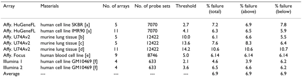
Page 4 of 24 (page number not for citation purposes) Table 2: Percentage of samples failing the Kolmogorov-Smirnov normality test

Array Materials No. of arrays No. of probe sets Threshold % failure

(total)

% failure (above)

% failure (below)

Affy. HuGeneFL human cell line SKBR [a] 5 7070 2.7 7.2 6.9 7.8

Affy. HuGeneFL human cell line IMR90 [a] 11 7070 4.1 6.3 6.5 5.9

Affy. U74Av2 murine lung tissue [b] 5 12422 10.0 6.1 6.6 5.5

Affy. U74Av2 murine lung tissue [c] 5 12422 13.6 7.6 8.3 6.4

Affy. U74Av2 murine lung tissue [d] 11 12422 14.2 10.6 10.6 10.7

Affy. Focus human blood cell line [e] 9 8746 5.0 6.14 6.14 6.14

Illumina 1 human cell line GM10469 [f] 4 633 2.1 4.6 3.9 6.2

Illumina 2 human cell line GM10469 [f] 4 633 3.6 6.5 6.6 6.2

Average --- --- --- --- 6.9 6.9 6.9

Percentage of samples failing the Kolmogorov-Smirnov normality test at the level P = 0.05. All arrays are normalized to 100% of the mean value. The columns %failure (above) and %failure (below) give percentage of failures above and below the specified threshold.

[a] data Ref. [10].

[b] C57BL/6 (B6) WT mice, data Ref. [15]. [c] C57BL/6-Cftr-/- KO inbred mice, data Ref. [15]. [d] data M. Cosio.

[e] data O. Modlich and S. Raschke. [f] lymphoblast cell line GM10469 [8].

Table 1: Illustration of the consecutive sampling procedure

Rank Probe set Sample Y1 Sample Y2 Y2-Y1 (Y2+Y1)/2 Sample Mean SD (Y2-Y1) SD(Y1)+ SD(Y2)

... ... ... ... ...

251 J03040_at 628 614 -14 621 614.4 71.1 71.8

252 M26880_at 657 583 -74 620

253 HG384-HT384_at 577 662 86 619

254 X04654_s_at 633 604 -29 619

255 J04046_s_at 554 680 126 617

256 X69908_rna1_at 593 640 47 617

257 D85758_at 672 555 -117 614

258 L12168_at 633 592 -41 612

259 HG1614-HT1614_at 590 633 43 611

260 X71428_at 571 649 77 610

261 S75463_at 602 615 13 608

262 X69910_at 579 630 50 604

263 X57346_at 597 610 13 603 590.1 136.2 137.0

264 U01691_s_at 576 630 54 603

265 X17620_at 605 594 -11 600

266 U10323_at 562 617 56 590

267 AJ001421_at 413 766 354 589

268 X62654_rna1_at 576 602 26 589

269 D64142_at 666 510 -156 588

270 D21063_at 562 613 51 588

271 X16560_at 588 580 -8 584

272 D26600_at 580 586 6 583

273 M19267_s_at 599 566 -33 583

274 J02621_s_at 688 475 -213 582

... ... ... ... ... ...

Rank shows the rank from the highest mean expression. The columns "Sample Y1 and Y2" give the expression values, Y2 - Y1 is the expressions

(5)

Page 5 of 24 (page number not for citation purposes) close to the mean D in a given range. The figures show

quantile-quantile plots (Q-Q plots), comparing the observed expression values to the corresponding values of the inverse normal cumulative distribution. The last panel D shows one sample that failed the test.

Furthermore, we observed that the probe sets with the mean expressions within a "reasonably small" range had, on average, a similar variance. Figure 2A shows pooled data of the 62 probe sets in the expression range from -0.1 to 0.1 (cell line IMR90, 11 replicates, Ref. [10]) in Q-Q plot in comparison to the inverse normal cumulative dis-tribution with good agreement except for about six out-liers. The picture changes when we scan probe sets with a wide range of mean expressions. Figure 2B shows the Q-Q plot of 185 probes sets in the range of means from 500 to 1000; the lower part of the graph deviates substantially from the straight line. When we plotted the relative expression (i.e. expressions of the individual probe sets divided by the mean of 11 arrays; Figure 2C), we got all the points, except for about ten outliers, back on the 45° line. This implies that the standard deviation is linearly proportional to the mean expression level.

Based on the evidence of Figure 2, we hypothesize that approximately the same standard deviation can be obtained by scanning the data vertically, i.e. looking at expressions of the neighboring probe sets, or horizontally, i.e. looking at the series of arrays for each probe set. In other words, the probability that we will observe a differ-ence d between the measurements M1 and M2 of the probe set Pr₁on the arrays A₁and A₂is, at least in the first approx-imation, about the same as the probability that we will observe such difference between the measurement M₃of the probe set Pr₁on the array A₁and the measurement M₄

of the probe set Pr₂on the array A₂, provided that the mean expression of both populations is the same. It fur-ther follows that an estimate of mean standard deviation of a group of genes with approximately same mean expression can be obtained from comparison of two arrays. We need to rank the probe sets according to the mean expression and evaluate the standard deviation from the differences in gene expressions in samples of k

consecutive genes; the range of the means within a sample must be small. Furthermore, in this arrangement we can also obtain the standard deviation by using the ranked probe sets of each individual array (Ref. [10], Supplemen-tary Material). Note that the standard deviation derived from the difference converges to √2σ, where σ is a stand-ard deviation of a given population. Figure 3 shows a comparison of the frequency distribution of the difference in expression of two consecutive samples with the corre-sponding inverse normal cumulative distribution (cell line IMR90).

Consecutive sampling analysis

Assume, as a working hypothesis, that we can estimate the standard deviation of the gene expression variability of series replicate arrays from two-array comparisons. Since the evidence derived from the frequency distribution sug-gests that the standard deviation is linearly proportional to the expression level (at least in the first approxima-tion), we assume that a representative estimate of the standard deviation can be obtained in the form of a linear function of the mean expression. A similar model was proposed on a basis of theoretical considerations by Rocke and coworkers [11-14]. The consecutive sampling program (see Methods) takes k pairs of expression values

Y_1iand Y_2iranked according to the mean (Y_1i, Y_2i) and cal-culates the standard deviation from the difference Y2i-Y1i, where the subscripts 1 and 2 denote the array number and

i signifies the probe set rank; typically we set k = 12, 25 or 50, depending on the size of the array. The standard devi-ation function is then determined by fitting the logarith-mically transformed values to the logarithm of the linear function of the mean expression (see the Methods sec-tion). For illustration, Figure 4A shows the dispersion plot and boundaries of the 0.8 and 0.95 probability intervals for the murine array MG U74Av2 (lung tissue, AKR mice; Table 4), whereas Figure 4B shows standard deviations of the consecutive samples consisting of 12 ordered pairs of probe sets and the regression curve, representing the standard deviation function.

(6)

Page 6 of 24 (page number not for citation purposes) points represent the standard deviations of the

expres-sions of individual probe sets and the solid line represents the standard deviation function derived from the consec-utive sampling.

Probability intervals and correlation of the Kαcoefficients

with t-distribution

Once we evaluate the standard deviation function, we can determine the limits of the probability intervals, i.e. the boundaries corresponding to a distance from the 45° axis of symmetry equal to a constant number of standard devi-ations. Equations defining these limits are given in the Methods section (Eqs. (2) and (3)). The coefficient Kαis equivalent to the standardized or "standard" deviate of the normal distribution, representing the distance from the mean, expressed in standard deviations. In case of the z-distribution or t-distribution the standard deviates cor-responding to specific probability intervals can be derived from the cumulative distribution function. Since the the-oretical distribution function corresponding to the proba-bility intervals of the microarray dispersion is unknown, we determined the coefficients Kαempirically. First we cal-culated the standard deviation function and then used Eqs. (2) and (3) to define the limits of the standard devi-ate intervals ("probability intervals"; see Figure 4A, note that the boundary lines appear in the log-log plot as curves). To determine the Kαcoefficients corresponding to specific probabilities we counted the points lying outside a given interval. For example, if the number of points in a given expression range examined was, say, 10000, we determined the K_α value corresponding to the interval 0.995 by finding the interval containing 9950 points (99.5%), leaving the 50 points outside. More precisely, the K_αis calculated as the average of the values corre-sponding to the integers above and below the number equal to the given fraction.

The Kαcoefficients are standardized with respect to the mean and standard deviation of given populations. As such, they are a universal measure of the probability of occurrence, function only of the shape of the distribution

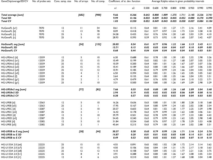
function. Considering the complexity of the processes involved in microarray experiments, we did not expect that the coefficient would be constant even for just a vari-ety of RNA samples of a given type of array. Nonetheless, examination of 42 microarray studies with two to 11 rep-licates comprising 682 arrays and 22 Affymetrix array types revealed that values of the K_αcoefficients were very close for all tested comparisons (note that multiple chip arrays are counted as multiple types). The coefficients were invariant for a wide range of dispersions, invariant with respect to different laboratory conditions, different tissues and different species and across all the types of arrays we tested. Table 4 shows a summary of the average values of Kαcoefficients for 900 pair-wise comparisons. The average coefficient a₁varied from 1.8 to 54.4 and coef-ficient a₂from 0.08 to 0.69, with total coefficients of vari-ation 1.05 and 0.54, respectively. In spite of such a wide range, the differences in the coefficient Kαwere small: the coefficient of variation ranged from the minimum 0.031 at the probability p = 0.9 to the maximum 0.101 at p = 0.995.

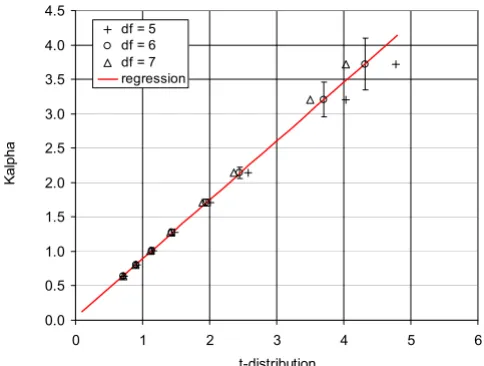
We examined the relationship between the coefficients K_α

and the inverse cumulative t-distribution. We found a very close linear correlation between the Kαvalues and the t-distribution values corresponding to the degree of free-dom df = 6. The adjusted R2 _{coefficient was 0.99993, with} the intercept of 0.039 and the coefficient of proportional-ity of 0.855. Figure 6 shows the graph of the Kαvalues plotted against the t-distribution parameters in the range of probability intervals from 0.5 to 0.995; the solid line represents the regression line for df = 6 and the bars indi-cate the standard deviation. We also compared directly the

K_αintervals and t-distribution. Figure 7 shows the proba-bility values corresponding to the Kαcoefficients and t- dis-tribution probability, represented by the solid curve. In the direct comparison we obtain better agreement for df = 12 than for df = 6.

A further examination of the results shown in Table 4 seemed to indicate that the older GeneChips® _{had a}

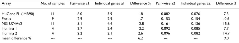
some-Table 3: Comparison of the coefficients of standard deviation function derived from the consecutive sampling and individual probe sets

Array No. of samples Pair-wise a1 Individual genes a1 Difference % Pair-wise a2 Individual genes a2 Difference %

HuGene FL (IMR90) 11 6.0 5.9 1.8 0.082 0.076 7.3

Focus 9 2.9 2.9 1.7 0.153 0.154 -0.6

MG-U74Av2 11 5.1 4.4 12.8 0.161 0.136 15.6

Illumina 1 4 2.7 2.4 12.2 0.092 0.085 7.7

Illumina 2 4 2.2 2.1 2.6 0.096 0.082 14.7

mean difference % --- --- --- 6.2 --- --- 9.0

(7)

Page 7 of 24 (page number not for citation purposes) what broader distribution. For example, the mean Kαat

0.995 for the array HuGene FL was 4.11, while these val-ues for the later versions HG-U95A and HG-U133A were 3.48 and 3.56, respectively. To assess the correlation between the developing technology and shape of the Kα distribution, we need a quantitative parameter, reflecting the technological advancement. One possibility is the fea-ture size and number of probe pairs per set, which have been systematically decreasing with time. Table 5 shows

the overview of the selected Kαvalues correlated with the technical factor TF, defined as the sum of the feature size and number of the probe pairs per probe set. In Figure 8 we present the K_αvalues at 0.95 and 0.995, plotted against TF. The regression line showed a slight decreasing ten-dency of the Kαvalues at 0.995 with the decreasing TF, but the graph was not very convincing; the adjusted R2 _was only 0.31. No trend was discernible at the probability of 0.95.

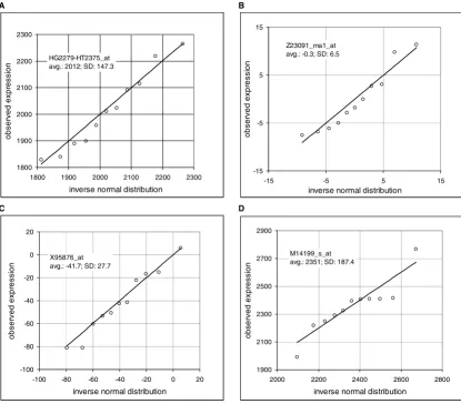
Comparison of the observed frequency distribution to the inverse normal cumulative distribution Figure 1

Comparison of the observed frequency distribution to the inverse normal cumulative distribution. Quantile-quantile plots show on y-axis the observed expression and on x-axis value of the corresponding inverse normal cumulative dis-tribution. Microarray data are derived from HuGeneFL, using IMR90 cell line with 11 samples. Panels show the probe sets with the Kolmogorov-Smirnov maximum distance D equal or close to the mean value in the specified average expression rage. Inserts provide the Affymetrix probe set identification, average expression for a given gene and standard deviation. A: probe set HG2279-HT2375_at, rank 43, expression range from 1000 to 6681 (high range, maximum), average D in the range is 0.176, sample D is 0.176; B: probe set Z23091_rna1_at, rank 5484, expression range from -0.4 to 0.4 (near-zero range), average D in the rang is 0.181, sample D is 0.182; C: probe set X95876_at, rank 7003, expression range from -20 to -923 (negative range, minimum), average D in the range is 0.183, sample D is 0.182; D: example of the probe set that failed the test – probe set M14199_s_at, rank 25, sample D is 0.204 (data Novak et al., IMR90 [10]).

A B

1800 1900 2000 2100 2200 2300

inverse normal distribution

ob

s

er

v

e

d ex

pr

es

s

ion

HG2279-HT2375_at avg.: 2012; SD: 147.3

-15 -5 5 15

o

b

s

e

rv

ed

ex

pr

es

si

o

n

Z23091_rna1_at avg.: -0.3; SD: 6.5

C D

-100 -80 -60 -40 -20 0 20

obs

er

ve

d ex

pr

es

si

on

X95876_at avg.: -41.7; SD: 27.7

1900 2100 2300 2500 2700 2900

2000 2200 2400 2600 2800

obser

ved ex

pr

essi

on

(8)

Page 8 of 24 (page number not for citation purposes) We found the probability intervals useful for estimating the significance of the observed differences, in particular in assays with small numbers of replicates (four or less). The Kαcoefficients representing the number of standard deviates that separates the measured values from the refer-ence mean values provide an objective measure of dissim-ilarity between the populations under consideration. For the single normal population the interpretation is straightforward. However, in case of the microarray data we deal with the multitude of populations and the theo-retical Kα function is unknown; our correlation results though indicate that a universal function, encompassing all GeneChip® _{types, exists. We could use the}_K_α_values obtained from correlations instead of the theoretical val-ues; however, the experience has shown that the results are not reliable. First, considering the large number of val-ues on the arrays even small differences in the Kαfunction translate into substantial differences in number of candi-dates. Second, quite frequently the unplanned differences between the samples cause deviations from the expected behavior and render comparison with the general func-tion unsuitable. Therefore, in practice, we use the Kα coef-ficients only for ranking.

To determine the best candidate genes differentially expressed, we search for the genes with the largest K_αin all or most of the comparisons. We named this method "con-secutive sampling and coincidence test." Briefly, we calcu-late the K_α coefficients in all possible N pair-wise comparisons and select the probe sets with expressions beyond a given probability interval in at least M compar-isons; the upper limit of probability of observing f false positives can be calculated theoretically, assuming ran-dom selection. Detailed discussion is beyond the scope of this study (a particular example of application to the anal-ysis of five-replicate assay of murine lung tissue can be found in Ref. [15]). The main advantages of this approach are that: 1) it is a nonparametric method; 2) applicable to assays with small number of replicates (as small as two); 3) it examines all pair-wise comparisons and makes easy to identify and automatically flag problematic arrays; 4) the probability of false positives can be easily calculated from the binomial distributions or estimated by straight-forward simulations [8]. Here, as a brief illustration of the consistency of this approach, Table 6a shows the analysis of five replicates of murine GeneChips MG-U74Av2, labeled as mg1 to mg5 (data Ref. [15]). The purpose is to examine consistency of the results of analysis of differen-tial expression using the t-test, coincidence method and RMA. For the test, we defined five subsets: [mg1, 2, 3, 4], [mg1, 2, 3, 5], [mg1, 2, 4, 5], etc. and selected the candi-date genes. The threshold of selection for the t-test was P = 0.01, for the coincidence 12 out of possible 16 cases, and for the RMA minimum fold difference 2. We selected the genes satisfying the given criteria for each subset and

Comparison of the observed frequency distribution to the inverse normal cumulative distribution, pooled data Figure 2

Comparison of the observed frequency distribution to the inverse normal cumulative distribution, pooled data. Quantile-quantile plots show on y-axis the observed expression and on x-axis value of the correspond-ing inverse normal cumulative distribution. Microarray data are derived from HuGeneFL, using the cell line IMR90 with 11 samples, pooled data. A: expression range from -0.1 to 0.1, 62 probe sets; B: expression range from 500 to 1000, 185 probe sets; C: expression range from 500 to 1000, 185 probe sets, relative expression values (sample expression divided by the mean of 11 samples; data Novak et al. [10]).

A

-30 -20 -10 0 10 20 30

-20 -10 0 10 20

ob

s

er

v

ed

ex

pr

es

s

ion

B

0 200 400 600 800 1000 1200 1400

0 200 400 600 800 1000 1200 1400 inverse normal distribution

obser

ved ex

p

ress

ion

C

0.0 0.2 0.4 0.6 0.8 1.0 1.2 1.4 1.6

0.6 0.8 1.0 1.2 1.4

obser

ved expr

ess

(9)

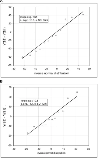
Page 9 of 24 (page number not for citation purposes) Comparison of the observed frequency distribution of consecutive samples to the inverse normal cumulative distribution Figure 3

Comparison of the observed frequency distribution of consecutive samples to the inverse normal cumulative distribution. Quantile-quantile plots show on y-axis the difference of expression of two microarrays and on x-axis value of the corresponding inverse normal cumulative distribution. Microarray data are derived from HuGeneFL, using cell line IMR90 [10]. Probe sets of the microarrays 1 and 3 are ordered according to the mean expression and statistical samples of 12 probe sets are taken in the range of ranks from 250 to 4800. Panels show the samples with the Kolmogorov-Smirnov maximum dis-tance equal or close to the mean value in the specified average expression rage. Inserts provide the average mean expression (range avg.), mean of the differences (s. avg.) and standard deviation (s. SD). A: expression range from 400 to 620, average D in the range is 0.142, sample D is 0.142; B: expression range from 10 to 20, average D in the range is 0.204, sample D is 0.204.

A

-80 -60 -40 -20 0 20 40 60

inverse normal distributioin

Y(

S3

)

Y(

S1

)

range avg.: 461

s. avg.: -13.8, s. SD: 35.5

B

-30 -20 -10 0 10 20 30

Y(

S3

)

Y(

S1

)

.

(10)

Biology Direct

2

006,

1

:27

http

://www.biol

ogy-di

rect.com/content/1/1/2

7

Pag

e 10 of

2

4

(page number not for citation purposes)

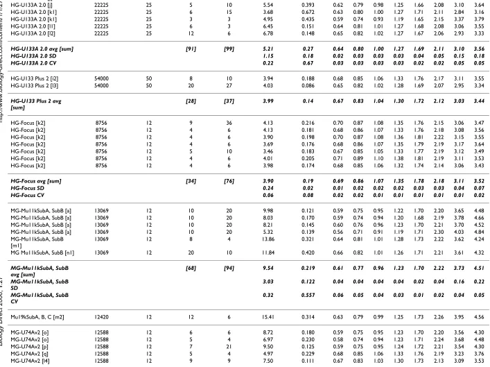
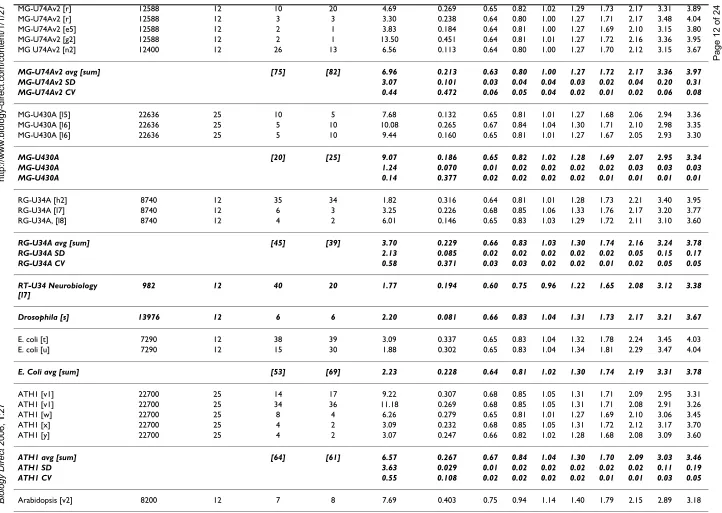
Table 4: Summary of values of the coefficients of standard deviation function and Kα coefficients

GeneChip/average/SD/CV No. of probe sets Cons. samp. size No. of arrays No. of comp. Coefficient. of st. dev. function Average Kalpha values in given probability intervals

a1 a2 0.500 0.600 0.700 0.800 0.900 0.950 0.990 0.995

Total average [sum] [682] [900] 9.66 0.266 0.642 0.808 1.009 1.275 1.711 2.145 3.226 3.741 Total SD 9.99 0.146 0.033 0.039 0.043 0.045 0.052 0.080 0.270 0.390 Total CV 1.03 0.550 0.052 0.049 0.043 0.035 0.030 0.037 0.084 0.104

HuGeneFL [a1] 7070 12 11 54 8.61 0.115 0.64 0.81 1.01 1.27 1.71 2.16 3.41 4.09

HuGeneFL [b] 7070 12 13 78 8.09 0.418 0.61 0.77 0.97 1.24 1.73 2.24 3.58 4.18

HuGeneFL [c] 7070 25 5 10 34.58 0.435 0.61 0.76 0.94 1.20 1.60 2.03 3.39 4.10

HuGeneFL [c] 7070 25 5 10 28.93 0.393 0.59 0.73 0.92 1.18 1.60 2.07 3.42 4.07

HuGeneFL avg [sum] [34] [152] 20.05 0.34 0.61 0.77 0.96 1.22 1.66 2.13 3.45 4.11 HuGeneFL SD 13.71 0.15 0.02 0.03 0.04 0.04 0.07 0.10 0.09 0.05

HuGeneFL CV 0.68 0.44 0.04 0.04 0.04 0.04 0.04 0.05 0.03 0.01

HG-U95Av2 [d] 12559 12 5 10 6.30 0.688 0.61 0.78 1.00 1.30 1.83 2.32 2.98 3.26

HG-U95Av2 [e1] 12559 25 15 15 10.49 0.199 0.65 0.82 1.01 1.27 1.68 2.07 3.05 3.55

HG-U95Av2 [e2] 12559 25 15 15 10.59 0.200 0.64 0.81 1.01 1.26 1.67 2.07 3.07 3.56

HG-U95Av2 [e3] 12559 25 15 15 10.41 0.189 0.63 0.80 1.00 1.25 1.66 2.07 3.06 3.55

HG-U95Av2 [e4] 12559 25 12 12 10.91 0.185 0.63 0.79 0.99 1.24 1.66 2.04 3.02 3.50

HG-U95Av2 [e5] 12559 25 4 2 6.50 0.394 0.65 0.82 1.01 1.26 1.65 2.05 3.05 3.62

HG-U95Av2 [f] 12559 25 4 2 5.64 0.155 0.64 0.81 1.00 1.25 1.66 2.04 2.92 3.31

HG-U95Av2 [g1] 12559 25 2 1 4.79 0.479 0.61 0.76 0.95 1.20 1.64 2.10 3.22 3.71

HG-U95Av2 [g1] 12559 25 5 10 3.31 0.500 0.64 0.80 1.00 1.26 1.69 2.09 2.98 3.29

HG-U95Av2 avg [sum] [77] [82] 7.66 0.33 0.63 0.80 1.00 1.26 1.68 2.09 3.04 3.48 HG-U95Av2 SD 2.94 0.19 0.02 0.02 0.02 0.03 0.06 0.09 0.08 0.16 HG-U95Av2 CV 0.38 0.57 0.02 0.02 0.02 0.02 0.04 0.04 0.03 0.05

HG-U95B [d] 12563 12 5 10 16.26 0.636 0.63 0.80 1.01 1.30 1.80 2.28 3.18 3.68

HG-U95B [e5] 12563 25 2 1 17.95 0.167 0.64 0.80 0.99 1.24 1.65 2.02 3.08 3.54

HG-U95C [d] 12587 12 5 10 20.57 0.603 0.64 0.81 1.02 1.30 1.77 2.25 3.39 3.98

HG-U95C [e5] 12587 25 2 1 16.42 0.178 0.63 0.79 0.99 1.23 1.62 2.00 3.06 3.61

HG-U95D [d] 12587 12 5 10 39.79 0.501 0.62 0.78 0.99 1.28 1.77 2.33 3.80 4.42

HG-U95D [e5] 12587 25 2 1 54.45 0.240 0.63 0.79 0.99 1.23 1.62 2.05 2.98 3.48

HG-U95E [d] 12582 12 5 10 31.84 0.534 0.60 0.76 0.97 1.27 1.78 2.29 3.53 4.08

HG-U95E [e5] 12582 25 2 1 45.64 0.215 0.63 0.79 1.00 1.25 1.64 2.02 2.88 3.31

HG-U95B to E avg [sum] [28] [44] 30.37 0.38 0.63 0.79 0.99 1.26 1.71 2.16 3.24 3.76 HG-U95B to E SD 14.87 0.20 0.01 0.01 0.02 0.03 0.08 0.14 0.31 0.37 HG-U95B to E CV 0.49 0.53 0.02 0.02 0.02 0.02 0.05 0.07 0.10 0.10

HG-U133A 2.0 [e6] 22225 25 15 15 4.55 0.091 0.65 0.82 1.02 1.28 1.72 2.14 3.14 3.62

HG-U133A 2.0 [e7] 22225 25 15 15 4.50 0.106 0.66 0.84 1.04 1.31 1.75 2.17 3.18 3.63

HG-U133A 2.0 [e8] 22225 25 12 12 4.10 0.108 0.67 0.84 1.05 1.32 1.77 2.21 3.26 3.75

HG-U133A 2.0 [h1] 22225 25 8 4 3.91 0.288 0.64 0.80 1.00 1.26 1.67 2.08 3.05 3.54

(11)

Biology Direct

2

006,

1

:27

http

://www.biol

ogy-di

7

Pag

e 11 of

2

4

HG-U133A 2.0 [j] 22225 25 5 10 6.54 0.390 0.62 0.79 0.98 1.25 1.68 2.10 3.13 3.62

HG-U133A 2.0 [j] 22225 25 5 10 5.54 0.393 0.62 0.79 0.98 1.25 1.66 2.08 3.10 3.64

HG-U133A 2.0 [k1] 22225 25 6 15 3.68 0.672 0.63 0.80 1.00 1.27 1.71 2.11 2.84 3.16

HG-U133A 2.0 [k1] 22225 25 3 3 4.95 0.435 0.59 0.74 0.93 1.19 1.65 2.15 3.37 3.79

HG-U133A 2.0 [l1] 22225 25 6 3 6.45 0.151 0.64 0.81 1.01 1.27 1.68 2.08 3.06 3.55

HG-U133A 2.0 [l2] 22225 25 12 6 6.78 0.148 0.65 0.82 1.02 1.27 1.67 2.06 2.93 3.33

HG-U133A 2.0 avg [sum] [91] [99] 5.21 0.27 0.64 0.80 1.00 1.27 1.69 2.11 3.10 3.56 HG-U133A 2.0 SD 1.15 0.18 0.02 0.03 0.03 0.03 0.04 0.05 0.15 0.18 HG-U133A 2.0 CV 0.22 0.67 0.03 0.03 0.03 0.03 0.02 0.02 0.05 0.05

HG-U133 Plus 2 [i2] 54000 50 8 10 3.94 0.188 0.68 0.85 1.06 1.33 1.76 2.17 3.11 3.55

HG-U133 Plus 2 [l3] 54000 50 20 27 4.03 0.086 0.65 0.82 1.02 1.28 1.69 2.07 2.95 3.34

HG-U133 Plus 2 avg [sum]

[28] [37] 3.99 0.14 0.67 0.83 1.04 1.30 1.72 2.12 3.03 3.44

HG-Focus [k2] 8756 12 9 36 4.13 0.216 0.70 0.87 1.08 1.35 1.76 2.15 3.06 3.47

HG-Focus [k2] 8756 12 4 6 4.13 0.181 0.68 0.86 1.07 1.33 1.76 2.18 3.08 3.56

HG-Focus [k2] 8756 12 4 6 3.90 0.198 0.70 0.87 1.08 1.36 1.81 2.22 3.15 3.55

HG-Focus [k2] 8756 12 4 6 3.69 0.176 0.68 0.86 1.07 1.35 1.79 2.19 3.17 3.64

HG-Focus [k2] 8756 12 5 10 3.46 0.183 0.67 0.85 1.05 1.33 1.77 2.19 3.12 3.49

HG-Focus [k2] 8756 12 4 6 4.01 0.205 0.71 0.89 1.10 1.38 1.81 2.19 3.11 3.53

HG-Focus [k2] 8756 12 4 6 3.98 0.174 0.68 0.85 1.06 1.32 1.74 2.14 3.06 3.43

HG-Focus avg [sum] [34] [76] 3.90 0.19 0.69 0.86 1.07 1.35 1.78 2.18 3.11 3.52

HG-Focus SD 0.24 0.02 0.01 0.02 0.02 0.02 0.03 0.03 0.04 0.07

HG-Focus CV 0.06 0.08 0.02 0.02 0.01 0.01 0.01 0.01 0.01 0.02

MG-Mu11kSubA, SubB [a] 13069 12 10 20 9.98 0.121 0.59 0.75 0.95 1.22 1.70 2.20 3.65 4.48

MG-Mu11kSubA, SubB [a] 13069 12 10 20 8.03 0.170 0.59 0.74 0.94 1.20 1.68 2.19 3.78 4.66

MG-Mu11kSubA, SubB [a] 13069 12 10 20 8.21 0.145 0.60 0.76 0.96 1.23 1.70 2.21 3.70 4.52

MG-Mu11kSubA, SubB [a] 13069 12 10 20 5.32 0.139 0.56 0.71 0.91 1.19 1.71 2.30 4.03 4.84

MG-Mu11kSubA, SubB [m1]

13069 12 8 4 13.86 0.321 0.64 0.81 1.01 1.28 1.73 2.22 3.62 4.24

MG Mu11kSubA, SubB [n1] 13069 12 20 10 11.84 0.420 0.66 0.82 1.01 1.26 1.71 2.21 3.61 4.32

MG-Mu11kSubA, SubB avg [sum]

[68] [94] 9.54 0.219 0.61 0.77 0.96 1.23 1.70 2.22 3.73 4.51

MG-Mu11kSubA, SubB SD

3.03 0.122 0.04 0.04 0.04 0.04 0.02 0.04 0.16 0.22

MG-Mu11kSubA, SubB CV

0.32 0.557 0.06 0.05 0.04 0.03 0.01 0.02 0.04 0.05

Mu19kSubA, B, C [m2] 12420 12 12 6 15.41 0.314 0.63 0.79 0.99 1.25 1.73 2.26 3.95 4.56

MG-U74Av2 [o] 12588 12 6 6 8.72 0.180 0.59 0.75 0.95 1.23 1.70 2.20 3.56 4.30

MG-U74Av2 [o] 12588 12 5 4 6.97 0.230 0.58 0.74 0.94 1.23 1.71 2.24 3.68 4.48

MG-U74Av2 [p] 12588 12 7 21 9.50 0.125 0.59 0.75 0.95 1.24 1.72 2.21 3.54 4.30

MG-U74Av2 [q] 12588 12 5 4 4.97 0.229 0.68 0.85 1.06 1.33 1.76 2.19 3.23 3.76

MG-U74Av2 [l4] 12588 12 9 9 7.50 0.111 0.67 0.83 1.03 1.30 1.73 2.13 3.09 3.53

(12)

Biology Direct

2

006,

1

:27

http

://www.biol

ogy-di

7

Pag

e 12 of

2

4

MG-U74Av2 [r] 12588 12 10 20 4.69 0.269 0.65 0.82 1.02 1.29 1.73 2.17 3.31 3.89

MG-U74Av2 [r] 12588 12 3 3 3.30 0.238 0.64 0.80 1.00 1.27 1.71 2.17 3.48 4.04

MG-U74Av2 [e5] 12588 12 2 1 3.83 0.184 0.64 0.81 1.00 1.27 1.69 2.10 3.15 3.80

MG-U74Av2 [g2] 12588 12 2 1 13.50 0.451 0.64 0.81 1.01 1.27 1.72 2.16 3.36 3.95

MG U74Av2 [n2] 12400 12 26 13 6.56 0.113 0.64 0.80 1.00 1.27 1.70 2.12 3.15 3.67

MG-U74Av2 avg [sum] [75] [82] 6.96 0.213 0.63 0.80 1.00 1.27 1.72 2.17 3.36 3.97 MG-U74Av2 SD 3.07 0.101 0.03 0.04 0.04 0.03 0.02 0.04 0.20 0.31 MG-U74Av2 CV 0.44 0.472 0.06 0.05 0.04 0.02 0.01 0.02 0.06 0.08

MG-U430A [l5] 22636 25 10 5 7.68 0.132 0.65 0.81 1.01 1.27 1.68 2.06 2.94 3.36

MG-U430A [l6] 22636 25 5 10 10.08 0.265 0.67 0.84 1.04 1.30 1.71 2.10 2.98 3.35

MG-U430A [l6] 22636 25 5 10 9.44 0.160 0.65 0.81 1.01 1.27 1.67 2.05 2.93 3.30

MG-U430A [20] [25] 9.07 0.186 0.65 0.82 1.02 1.28 1.69 2.07 2.95 3.34

MG-U430A 1.24 0.070 0.01 0.02 0.02 0.02 0.02 0.03 0.03 0.03

MG-U430A 0.14 0.377 0.02 0.02 0.02 0.02 0.01 0.01 0.01 0.01

RG-U34A [h2] 8740 12 35 34 1.82 0.316 0.64 0.81 1.01 1.28 1.73 2.21 3.40 3.95

RG-U34A [l7] 8740 12 6 3 3.25 0.226 0.68 0.85 1.06 1.33 1.76 2.17 3.20 3.77

RG-U34A, [l8] 8740 12 4 2 6.01 0.146 0.65 0.83 1.03 1.29 1.72 2.11 3.10 3.60

RG-U34A avg [sum] [45] [39] 3.70 0.229 0.66 0.83 1.03 1.30 1.74 2.16 3.24 3.78

RG-U34A SD 2.13 0.085 0.02 0.02 0.02 0.02 0.02 0.05 0.15 0.17

RG-U34A CV 0.58 0.371 0.03 0.03 0.02 0.02 0.01 0.02 0.05 0.05

RT-U34 Neurobiology [l7]

982 12 40 20 1.77 0.194 0.60 0.75 0.96 1.22 1.65 2.08 3.12 3.38

Drosophila [s] 13976 12 6 6 2.20 0.081 0.66 0.83 1.04 1.31 1.73 2.17 3.21 3.67

E. coli [t] 7290 12 38 39 3.09 0.337 0.65 0.83 1.04 1.32 1.78 2.24 3.45 4.03

E. coli [u] 7290 12 15 30 1.88 0.302 0.65 0.83 1.04 1.34 1.81 2.29 3.47 4.04

E. Coli avg [sum] [53] [69] 2.23 0.228 0.64 0.81 1.02 1.30 1.74 2.19 3.31 3.78

ATH1 [v1] 22700 25 14 17 9.22 0.307 0.68 0.85 1.05 1.31 1.71 2.09 2.95 3.31

ATH1 [v1] 22700 25 34 36 11.18 0.269 0.68 0.85 1.05 1.31 1.71 2.08 2.91 3.26

ATH1 [w] 22700 25 8 4 6.26 0.279 0.65 0.81 1.01 1.27 1.69 2.10 3.06 3.45

ATH1 [x] 22700 25 4 2 3.09 0.232 0.68 0.85 1.05 1.31 1.72 2.12 3.17 3.70

ATH1 [y] 22700 25 4 2 3.07 0.247 0.66 0.82 1.02 1.28 1.68 2.08 3.09 3.60

ATH1 avg [sum] [64] [61] 6.57 0.267 0.67 0.84 1.04 1.30 1.70 2.09 3.03 3.46

ATH1 SD 3.63 0.029 0.01 0.02 0.02 0.02 0.02 0.02 0.11 0.19

ATH1 CV 0.55 0.108 0.02 0.02 0.02 0.02 0.01 0.01 0.03 0.05

Arabidopsis [v2] 8200 12 7 8 7.69 0.403 0.75 0.94 1.14 1.40 1.79 2.15 2.89 3.18

(13)

Biology Direct

2

006,

1

:27

http

://www.biol

ogy-di

7

Pag

e 13 of

2

4

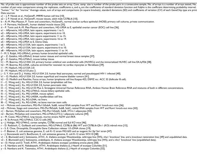
No. of probe sets is approximate number of the probe sets on array, Cons. samp. size is number of the probe pairs in a consecutive sample, No. of arrays is a number of arrays tested, No. of comp. is the number of pair-wise comparisons among the replicates, coefficients a1 and a2 are the coefficients of standard deviation function and Kalpha is the coefficient determining probability interval; "h." stands for

"human," "m." for "murine." Average values, sum of arrays and comparisons (in square brackets), standard deviations (SD) and coefficients of variation (CV) of each GeneChip type are printed in bold italics. Data sources:

a1 – J. P. Novak et al., HuGeneFl, IMR90 human cell line [10].

a2 – J. P. Novak et al., HuGeneFl, mouse tissues, adult male C57BL/6 [10].

b – A.-M. Mes-Masson, P. Tonin and coworkers, HuGeneFL, normal ovarian surface epithelial (NOSE) primary cell cultures, private communication. c – P. Permana, HuGeneFL, human skeletal muscle tissue [35].

d – P. Tonin and A.-M. Mes-Masson and coworkers, HG-U95A to E, epithelial ovarian cancer (EOC) cell line [36]. e1 – Affymetrix, HG-U95A, latin square, experiments 1 to 5.

e2 – Affymetrix, HG-U95A, latin square, experiments 6 to 10. e3 – Affymetrix, HG-U95A, latin square experiments 11 to 15. e4 – Affymetrix, HG-U95A, latin square, experiments 16 to 19. e5 – Affymetrix, HG-U95A to E, Demo Data.

e6 – Affymetrix, HG-U133A, latin square, experiments 1 to 5. e7 – Affymetrix, HG-U133A, latin square, experiments 6 to 10. e8 – Affymetrix, HG-U133A, latin square, experiments 11 to 14. f – M. S. Rolph, HG-U95Av2, primary human bronchial epithelial cells.

g1 – Z. Gatalica, HG-U95Av2, breast tumor tissues and normal breast tissue samples [37]. g2 – Z. Gatalica, MG-U74Av2, mouse kidney tissue.

h1 – M. Boerma, HG-U133A 2.0, primary human umbilical vein endothelial cells (HUVECs) and the immortalized HUVEC cell line EA.hy926 [38]. h2 – M. Boerma, RG-U34A, cultures enriched for neonatal rat cardiac myocytes or fibroblasts [39].

i1 – M. Hajduch, HG-U133A 2.0. i2 – M. Hajduch, HG-U133 plus 2.

j – S. Y. Kim and D. J. Volsky, HG-U133A 2.0, human fetal astrocytes, normal and pseudotyped HIV-1 infected [40]. k1 – O. Modlich, HG-U133A 2.0, human superficial and invasive bladder tumors [41].

k2 – O. Modlich and Raschke, Focus arrays, human lymphoma cell line Kaspas-422, DSMZ no.: ACC 32 (follicular B cell). l1 – C. Wang and J. Xu, HG-U133A 2.0, human lymphoblast cell line.

l2 – C. Wang and J. Xu, HG-U133A 2.0, human pancreatic islet.

l3 – C. Wang and J. Xu, HG-U133 Plus 2, Stratagene Universal Human Reference RNA, Ambion Human Brain Reference RNA and mixtures of both in different concentrations. l4 – C. Wang and J. Xu, MG-U74Av2, mouse biliary epithelial cells.

l5 – C. Wang and J. Xu, MG-U430A, mouse spleen. l6 – C. Wang and J. Xu, MG-U430A, myofibroblast cell line. l7 – C. Wang and J. Xu, RG-U34A, rat livers.

l8 – C. Wang and J. Xu, RG-U34A, rat bone marrow stem cells.

m1 – McInnes and coworkers, MG-Mu11kSubA, SubB, retinal RNA samples from WT and Rom1 knock-out mice [36].

m2 – McInnes, Szego and coworkers, MG-Mu19kSubA, SubB, SubC, retinal RNA samples from WT and Rom1 knock-out mice [42]. n1 – Burton, McGehee and coworkers, MG-Mu11kSubA, SubB, 3T3-L1 adipocytes [43].

n2 – Burton, McGehee and coworkers, MG-U74Av2,3T3-L1 adipocyte cultures [44]. o – M. Cosio, MG-U74Av2, lung tissues, murine strains NZW and AKR.

p – R. St-Arnaud, MG-U74Av2, C2C12 cells [45].

q – J. Hidalgo, MG-U74Av2, cortex samples, C57B6 normal and IL6 KO mice [46].

r – D. Radzioch, C. Guilbault and coworkers, MG-U74Av2, C57BL/6 (B6) WT and C57BL/6-Cftr-/- (KO) inbred mice [15]. s – S. E. Choe, Drosophila, Drosophila Gene Collection release 1.0 cDNA clones [19].

t – F. Blattner, E. coli antisense genome, E. coli K-12 strain MG1655 and an isogenic fnr::Spr _Smr _{strain [47].}

u – J. Slonczewski and S. BonDurant, E. coli antisense genome, E. coli K-12 strain W3110 [48].

v1 – E. Blumwald and J. Sottosanto, ATH1, A. thaliana ecotype Wassilewskija, wild-type line (WS), nhx1 'knockout' line, and a knockout restoration line; [49] and unpublished data. v2 – E. Blumwald and J. Sottosanto, arabidopsis, A. thaliana ecotype Wassilewskija, wild-type line (WS), and a nhx1 'knockout' line (unpublished data).

w – D. Honys and D. Twell, ATH1, Arabidopsis thaliana ecotype Landsberg erecta plants [50]. x – E. Nambara and K. Nakabayashi, ATH1, Arabidopsis thaliana (L.) Heynh of ecotype Columbia [51]. y – E. Nambara and K. Tatematsu, ATH1, Arabidopsis thaliana (L.) Heynh of ecotype Columbia [52].

(14)

Page 14 of 24 (page number not for citation purposes) subsequently counted the common genes found in any

two particular subsets. The mean values of all possible comparisons are shown in the fourth row of Table 6a. The values shown in the last row represent the ratio of the mean number of common genes relative to the mean number of the genes that passed the test for each subset (third row) in percent. In the case of the t-test, the average for the over- and under-expressed genes was 23 and 29 percent, respectively. By comparison, the coincidence test for the over-expressed genes yielded 75% and RMA 81%; in the case of the coincidence and RMA, the mean num-bers of under-expressed genes were below ten and the

comparisons were considered unreliable (data not shown). In only this example we used MAS 5 generated values. Table 6b shows the results of similar tests carried out using the Illumina fiberoptic bead-based oligonucle-otide arrays. In this case the average percentages of agree-ment for the coincidence tests were 89.1, to compare to 48.2%, obtained for the t-test. A more detailed compari-son under slightly different assumptions, which includes also the CyberT and Tusher's method, can be found in Ref. [8].

Discussion

In our practice we adopted the approach of Affymetrix, which estimates the background from 2% of the probes with the lowest signals, uses the MM probes for the mate of the non-specific component and yields an esti-mate of an "absolute" value of the RNA abundance. We adhered to the Affymetrix philosophy in spite of popular-ity of the global fitting methods, such as dChip [3,4] and RMA [6,7], because it provide us with a representative expression values independently for each array, enables us to assess consistency of the observed values and detect irregularities and outliers. This is an important advantage, considering how frequently we detect "atypical" arrays among replicates. Furthermore, consistency checks have

Standard deviation of the Focus arrays, arrays 01 to 09 Figure 5

Standard deviation of the Focus arrays, arrays 01 to 09. Standard deviations are calculated from the individual probe sets of nine samples. The solid curve represents the standard deviation function derived from the consecutive sampling. The regression curve corresponding to logarithm of the linear standard deviation function fitted to logarithm of the experimental standard deviation (not shown) overlaps the consecutive sampling approximation; the coefficients obtained from consecutive sampling are a₁= 2.92√2 and a₂= 0.153√2 and the regression coefficients obtained from indi-vidual probe sets are a1 = 2.87 and a2 = 0.154 (data Modlich,

Focus 1). 0.1 1.0 10.0 100.0 1000.0

0.1 1.0 10.0 100.0 1000.0 10000.0 Yavg

SD

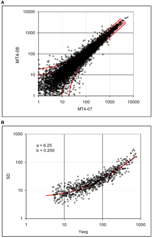
Dispersion of the murine tissue data, array MG-U74Av2, samples MT4-07 and MT4-08

Figure 4

Dispersion of the murine tissue data, array MG-U74Av2, samples MT4-07 and MT4-08. A. Dispersion plot and boundaries of the 0.8 and 0.95 probability intervals.

B: Standard deviations calculated using the expression differ-ence in consecutive samples and the regression curve (solid line), representing the standard deviation function (data Cosio).

A

1 10 100 1000 10000

MT4-07

M

T

4-08

.

B

1 10 100 1000

Yavg

SD

(15)

Page 15 of 24 (page number not for citation purposes) shown similar rates of coincidence for both RMA and coincidence testing (Table 6a).

Results of the published studies comparing various meth-ods of analysis are inconsistent and do not provide a clear guidance for selection of the method. Irizarry et al. [7], e.g., reported better detection of differentially expressed genes by RMA as compared to the dChip [4] and Affyme-trix "Average Difference" (MAS 4) and MAS5 methods. Similarly, Barash et al. rated RMA as the best of the three with dChip performing slightly better than MAS5 [16]. Shedden et al. [17] claim superior results for dChip and "trimmed mean" and inferior results for MAS5 and one version of RMA (GCRMA-EB); the other version of RMA (CGRMA-MLE; Wu Z, Irizarry R, Gentleman R, Murillo F, Spencer F., 2003, A Model Based Background Adjustment for Oligonucleotide Expression Arrays, Technical Report, John Hopkins University, Department of Biostatistics Working Papers, Baltimore, MD) produced mixed results (in trimmed mean the PM-MM differences are ordered, 20% of the highest and lowest values are deleted and the mean of the remaining probe pairs represents a measure of gene expression). Han et al. [18] compared the Affyme-trix MAS 5, dChip using PM-MM and PM only input and RMA. In this study the PM only variant of dChip and RMA showed the best performance. The authors also noted that the coefficient of variation in replicate experiments in the case of MAS 5 increases with a decreasing mean signal, but remains approximately constant for PM only of dChip and RMA. Invariance of the coefficient of variation raises a certain concern: percentage of contribution of the non-specific signal increases with the decreasing concentration and one would expect that at low concentrations it would be harder to separate it from the specific component. Choe et al. [19] compared various combinations of the six steps in the differential expression analysis: background subtraction, probe-level normalization, PM adjustment (correction for the non-specific signal), expression sum-mary (derivation of the representative gene expression from the multiple probe signals), probe set-level normal-ization and statistical evaluation. This was a particularly interesting comparative study, since their experimental design was much closer to real conditions than spiked sets of arrays used in other publications. The authors report that the combination of the MAS5 for background correc-tion and PM adjustment, median Polish method or, mar-ginally inferior, MAS5 for expression summary, loess for normalization and CyberT for statistical evaluation [20] yielded the best results. They also emphasized that, under their particular conditions, MM signals provided the best estimate of the non-specific component. Furthermore, they concluded that in the statistical evaluation it is important to account for variation of the standard devia-tion with the mean expression (see also [21]). They adopted the CyberT model proposed by Baldi and Lang

Comparison of the Kαdistribution and inverse t-distribution

Figure 7

Comparison of the Kαdistribution and inverse t -dis-tribution. K_αvalues correspond to probabilities from 0.5 to 0.995. The degree of freedom for the inverse t-distribution (solid lines) is 6 and 12.

0.0 0.1 0.2 0.3 0.4 0.5 0.6

0 1 2 3 4 5

Kalpha, t-distribution

p

ro

b

a

b

ilit

y

Kalpha df = 12 df = 6

Correlation of the K_αcoefficients and inverse t-distribution

Figure 6

Correlation of the K_αcoefficients and inverse t -distri-bution. Figure shows the values of K_αcoefficient correlated with the corresponding values of the t-distribution in the range of probabilities from 0.5 to 0.995. The adjusted R2

coefficient is 0.99993, intercept is 0.039 and the coefficient of proportionality is 0.855. The degree of freedom for the t -dis-tribution is 6.

0.0 0.5 1.0 1.5 2.0 2.5 3.0 3.5 4.0 4.5

0 1 2 3 4 5 6

t-distribution

Ka

lp

h

a

(16)

Page 16 of 24 (page number not for citation purposes) [20], which uses consecutive samples to estimate the

expression-dependent component of the standard devia-tion, similarly to our approach.

In the present analysis of the frequency distributions and properties of the Kαwe used the MAS 4 software, instead of MAS 5 or GCOS. The reason is that these more recent versions distort the frequency distribution and standard

deviation function in the near-zero region. In the case of the Affymetrix arrays the estimate of additive signal, caused by nonspecific binding and other spurious phe-nomena, is based on the mismatch signal. The estimate of the "true" gene expression is then derived from the differ-ence between perfect match (PM) and mismatch (MM). However, in such system the variability of this difference is a "true" measure of the absolute gene expression varia-bility. Negative difference does not mean that the gene expression is negative, but simply that the MM signal is larger than PM. It is perfectly logical that in absence of a given RNA the MM signal would exceed PM in about 50% of cases. The frequency distribution of the PM – MM dif-ference in the absence of a specific RNA is the best meas-ure of the constant component of spurious signal, added to the "true signal" value. Such estimate cannot be derived from MAS 5 or GCOS data. Replacing the negative values resulting from the signals actually measured by the PM and MM probes by arbitrary numbers introduces incon-sistency in the method of evaluation and leads to decrease of the standard deviation with decreasing signal level in near-zero region (unpublished observation). In the low expression region it also leads to a substantial increase in number of probe sets that deviate from the normal distri-bution [22]. Nevertheless, at the expression levels above about 50 (normalized to 100% of the mean) our observa-tions and conclusions hold even for the data analyzed with MAS 5 or GCOS. Some methods of analysis, such as RMA and one variant of the dChip, avoid the negative val-ues without introducing inconsistency in evaluation by using the PM values only.

Average Kαcoefficients at the intervals 0.95 and 0.995

Figure 8

Average Kαcoefficients at the intervals 0.95 and 0.995. Correlation of the K_αcoefficients with the sum of the feature size and number of probe pairs; bars show the stand-ard deviation for the interval 0.995.

0.0 0.5 1.0 1.5 2.0 2.5 3.0 3.5 4.0 4.5 5.0

20 25 30 35 40 45 50

TF

Ka

lp

h

a

probability 0.995 probability 0.95 regression

Table 5: Overview of the GeneChip types

GeneChip Feature size Probe pairs TF No. of labs. No. of arrays Ka 0.95 Ka 0.99 Ka 0.995

avg SD avg SD avg SD

HuGeneFL 24 20 44 2 34 2.13 0.10 3.45 0.09 4.11 0.05

HG-U95Av2 20 16 36 4 77 2.09 0.09 3.04 0.08 3.48 0.16

HG-U95B to E 20 16 36 2 28 2.16 0.14 3.24 0.31 3.76 0.37

HG-U133A 2.0 11 11 22 6 91 2.11 0.05 3.10 0.15 3.56 0.18

HG-U133 Plus 2 11 11 22 2 28 2.12 --- 3.03 --- 3.44

---HG-Focus 18 11 29 1 34 2.18 0.03 3.11 0.04 3.52 0.07

MG-Mu11kSubA, SubB 24 20 44 2 80 2.22 0.04 3.73 0.16 4.52 0.20

Mu19kSubA, B, C 24 20 44 1 12 2.26 --- 3.95 --- 4.56

---MG-U74Av2 20 16 36 6 75 2.17 0.04 3.36 0.20 3.97 0.31

MG-U430A 11 11 22 1 20 2.07 0.03 2.95 0.03 3.34 0.03

RG-U34A 24 16 40 2 45 2.16 0.05 3.24 0.15 3.78 0.17

RT-U34 Neurobiology 24 16 40 1 40 2.08 --- 3.12 --- 3.38

---Drosophila 20 14 34 1 6 2.17 --- 3.21 --- 3.67

---E. Coli 24 15 39 2 53 2.19 --- 3.31 --- 3.78

---ATH1 18 11 29 4 64 2.09 0.02 3.03 0.11 3.46 0.19

Arabidopis [s2] 24 16 40 1 7 2.15 --- 2.89 --- 3.18

---The first two columns of data show the feature size and number of the probe pairs per probe set. TF is the technical factor defined as the sum of feature size and probe pairs. No. of lab gives the number of different laboratories, where the data were generated. No. of arrays gives the number

(17)

Page 17 of 24 (page number not for citation purposes) In the preceding section, we demonstrated that the

fre-quency distribution of the random and pseudo-random fluctuations of microarray data is predominantly normal. The normal frequency distribution is a useful property, allowing straightforward identification of outliers, a con-venient quality check and simple characterization of the observed data. Normality of the error term is an important assumption of various global models used for the analysis of measured probe signals, such as dChip [3,4], RMA [5-7] and other approaches [23-25]. Among these only Pavelka et al. [25] demonstrated that the assumption is justified. Normality is also a necessary condition for appli-cation of the parametric methods. Here we observed that on average over 5% of samples deviate from the normal distribution (using the test threshold of 0.05). It is agreed that the t-test and ANOVA are rather robust with respect to normality (e.g. SigmaStat software [SPSS inc.] uses for ANOVA the threshold of 0.01), nonetheless the noted deviations call for caution when using parametric meth-ods, in particular considering that every analysis involves multiple testing. Our conclusion differs from that of Gilles and Kipling [22], who studied normality of Gene-Chip data using a set of 59 Affymetrix HG-U95A microar-rays with human pancreatic cRNA. The authors concluded that "...data provide strong support for the application of parametric tests to GeneChip data sets without the need for data transformation." However, Shapiro-Wilks test, applied to the MAS 4 evaluated data, detected 28% of probe sets deviating from normality at the level P < 0.05. The authors argued that the Shapiro-Wilks test is, perhaps, too sensitive, since the Q-Q plots of the observed and

nor-mal values show high correlation. In our opinion, correla-tion is not a reliable measure of normality. The correlacorrela-tion coefficient can be high in spite of a small number of out-lying points that might sufficiently affect variance to lead to false positive conclusions. Gilles and Kipling also observed an excessively high percentage of deviations from normality at low expression levels in data evaluated using MAS 5 and deduced that the most likely reason is MAS 5 treatment of negative values.

The probability of any value in normally distributed pop-ulations can be expressed as a number of standard devi-ates. For example, expressing the difference between the mean of a given population and a particular measurement in standard deviates enables us to compare this difference to the standardized z-distribution and determine, among other things, the cumulative probability of occurrence. For example, the standard deviate of 3.09 corresponds to the cumulative probability of measurements in the tails of the distribution function P = 0.001, a conventional threshold for identifying outliers in small-size samples. In the case of microarrays, we do not have single standard deviate values but standard deviate functions, defined by the K_α coefficients. Nonetheless, the same reasoning applies. The necessary and sufficient condition for "stand-ardization" of microarray dispersion is that the K_α coeffi-cients must be invariant. Under such condition differences expressed in Kαvariable are universal, inde-pendent of the particular properties of RNA samples, type of array, etc. This is of a practical significance for compar-ative studies, such as studies comparing results obtained

Table 6: Summary of the results of consistency tests

a)

t-test: P < 0.010 Coincidence RMA

Above or Below above below above above

Mean of 4-sample test 58.2 72.0 29.4 40.4

Common to 2 sets (mean) 13.5 20.5 22.1 32.9

SD 2.3 2.8 3.4 6.0

Ratio % 23.2 28.5 75.2 81.4

b)

Coincidence, interval 0.9 Coincidence, interval 0.8 t-test P = 0.0016

Mean of 3-samples test (7 of 9) 12.3 17.5 11.0

Common to 2 sets (average) 10.2 16.7 5.3

Ratio (%) 83.0 95.2 48.2

a) The t-test, coincidence test and RMA on MG-U75Av2 array (five samples; data Ref. [15]). The data were subject to one-tail t-test at the level

0.01, coincidence test and RMA. The coincidence and RMA tests were not carried out for the cases below the interval, since the numbers of occurrences were too small. The means of positive cases in five four-sample tests are given. The means of genes common to any two trials are

shown. Ratio of the means is given in percent. b) The t-test and coincidence test, Illumina (four samples; data Ref. [8]). The second and third

(18)

Page 18 of 24 (page number not for citation purposes) in different laboratories [26-28], different generations of

the Affymetrix array [29,30] or in different species [31-34].

Analysis of significance in assays with less than five repli-cates always represents a problem. Parametric methods are not reliable in the case of small samples and the non-parametric Mann-Whitney test and ANOVA on ranks pro-vide a very crude estimate for three or four samples and are not very reliable either. Before asserting the invariance of Kαvalues, we used probability intervals in pair-wise case-control comparisons and selected as candidate genes the genes that fell outside a given interval in predeter-mined number of comparisons [8,15]. We refer to this method as the "consecutive sampling and coincidence test." A more appropriate approach would be to estimate

Kαcoefficients representing the random variability from replicate arrays and apply the coincidence test to the ini-tial sets of genes lying outside the intervals defined by these values.

Besides the significance estimates, we found that the prob-ability intervals determined by Kαcoefficients are very use-ful for filtering out the random probe sets prior to the clustering analysis, in particular when hierarchical cluster-ing o