R E S E A R C H A R T I C L E
Open Access
Estimating the basic reproduction number
for single-strain dengue fever epidemics
Adnan Khan
1, Muhammad Hassan
2and Mudassar Imran
1*Abstract
Background: Dengue, an infectious tropical disease, has recently emerged as one of the most important
mosquito-borne viral diseases in the world. We perform a retrospective analysis of the 2011 dengue fever epidemic in Pakistan in order to assess the transmissibility of the disease. We obtain estimates of the basic reproduction number R0from epidemic data using different methodologies applied to different epidemic models in order to evaluate the robustness of our estimate.
Results: We first estimate model parameters by fitting a deterministic ODE vector-host model for the transmission dynamics of single-strain dengue to the epidemic data, using both a basic ordinary least squares (OLS) as well as a generalized least squares (GLS) scheme. Moreover, we perform the same analysis for a direct-transmission ODE model, thereby allowing us to compare our results across different models. In addition, we formulate a direct-transmission stochastic model for the transmission dynamics of dengue and obtain parameter estimates for the stochastic model using Markov chain Monte Carlo (MCMC) methods. In each of the cases we have considered, the estimate for the basic reproduction numberR0is initially greater than unity leading to an epidemic outbreak. However, control measures implemented several weeks after the initial outbreak successfully reduceR0to less than unity, thus resulting in disease elimination. Furthermore, it is observed that there is strong agreement in our estimates for the pre-control value ofR0, both across different methodologies as well across different models. However, there are also significant differences between our estimates for the post-control value of the basic reproduction number across the two different models. Conclusion: In conclusion, we have obtained robust estimates for the value of the basic reproduction numberR0 associated with the 2011 dengue fever epidemic before the implementation of public health control measures. Furthermore, we have shown that there is close agreement between our estimates for the post-control value ofR0 across the different methodologies. Nevertheless, there are also significant differences between the estimates for the post-control value ofR0across the two different models.
Keywords: Epidemiology, Dengue fever, Statistical inference, Stochastic model, Markov chain Monte Carlo
Multilingual abstracts
Please see Additional file 1 for translations of the abstract into the six official working languages of the United Nations.
Background
Global incidence of dengue has seen a striking increase over the past few decades [1,2]. The infectious disease is now endemic in more than a hundred tropical and
*Correspondence: [email protected]
1Department of Mathematics, Lahore University of Management Sciences, DHA, Lahore, Pakistan
Full list of author information is available at the end of the article
subtropical countries worldwide [1-3]. With an estimated 50–100 million cases and nearly 10,000- 20,000 deaths annually, dengue ranks second to Malaria amongst deadly mosquito-borne diseases [1,2,4-6]. The disease is caused by one of four virus serotypes (strains) of the genus
Flavivirus [2,3,7]. Most infected individuals suffer from dengue fever, a severe flu-like illness characterized by high fever, which is not usually a threat to mortality [2,8]. The symptoms of the disease last one to two weeks, after an initial incubation period of about 4–7 days [9]. Some infected individuals however, develop dengue hem-orrhagic fever (DHF) resulting in bleeding, low levels of blood platelets and blood plasma leakage, or dengue shock
syndrome (DSS) resulting in extremely low blood pres-sures. The risk associated with DHF and DSS is consider-ably higher, with mortality ranging from 5–15% [3,5,9,10]. There is evidence of dengue epidemics occurring in North America, Asia and Africa in the late 18thcentury [3]. Up until the middle of the 20th century however, incidences of dengue fever have been rare [3]. Nonethe-less, since the 1970’s, there has been a marked increase in the number of dengue cases, as well as the frequency and severity dengue epidemics, with the WHO claiming a 30-fold increase in the incidence of dengue between 1960 and 2010 [2,3,8]. Factors such as population growth, rapid urbanization and increase international travel are often cited as having contributed to this dramatic increase [8]. Dengue is currently endemic in nearly 110 countries in Southeast Asia, the Americas, Africa and the Eastern Mediterranean [2]. The WHO estimates that nearly 2.5 billion people are at risk of contracting the disease. Fur-thermore, nearly 50–100 million cases and almost 20,000 deaths due to more severe forms of dengue fever are reported globally every year, making dengue one of the deadliest mosquito-transmitted diseases [1,2,4-6].
Dengue is transmitted to humans through mosquito
bites. Female mosquitos of the Aedas genus, primarily
Aedes aegypti, acquire the dengue virus through a blood meal from infected humans [2,11]. The dengue virus has an incubation period of about 7–10 days in the vector, and is then spread to susceptible humans who are bit-ten by the infected mosquito [9]. The virus also has an incubation period of 4–7 days in the host [9]. While vec-tors never recover from infection with the dengue virus, the infection in hosts lasts only about one to two weeks [2]. Hosts that recover from infection with one serotype of the dengue virus gain life-long immunity from that serotype but only temporary and partial immunity to other serotypes [2,4,12-14]. This partial cross-immunity is the cause of antibody-dependent enhancement (ADE) in the setting of a secondary infection with a different serotype of DENV (Dengue Virus). ADE is hypothesized to be one factors leading to DHF and DSS, the more severe form of dengue disease [4,12,13,15]. In this study however, we will consider infection involving only a single serotype of the dengue virus.
About 80% of individuals suffering from a primary infec-tion with DENV are asymptomatic or display only a mild, uncomplicated fever [2,8]. A much smaller proportion of infected individuals suffer from dengue hemorrhagic fever and dengue shock syndrome [3,5,9]. As mentioned previ-ously however, risk of DHF and DSS is associated primar-ily with secondary infection with a heterologous serotype of DENV [4,12,13,15]. In general, the course of infection of dengue can be divided into three separate phases: febrile, critical and recovery. The febrile phase, which is rarely life threatening, is marked by the sudden onset of high fever,
rash, headaches and muscle and joint pains, which lead to the alternative name "breakbone fever" for dengue disease [8]. While most individuals then progress to the recov-ery phase, a small fraction of infected individuals instead progress to the critical phase of the disease. This phase lasts for one or two days and is marked by low blood pressure, leakage of blood plasma from the capillaries and decreased blood supply to organs. Severe cases of these symptoms are associated with DHF and DSS and the mor-tality in this phase of the disease is estimated to be as high as 5–15% [3,5,8,9].
Over the past several years, a number of deterministic mathematical models have been proposed to analyze the transmission dynamics of dengue in urban communities [5,11-17]. L. Esteva and C. Vargas [14] have investigated the coexistence of two serotypes of dengue virus using a deterministic ODE model. Moreover, Ferguson et al. [15] have investigated the effects of ADE on the transmission of multiple serotypes of dengue virus. In addition, Garba et al. [11] have shown the existence of a backward bifur-cation in a standard incidence ODE model for a single strain of dengue virus. Garba et al. [12] have also explored the effects of cross-immunity on the transmission dynam-ics of two strains of dengue virus. Similarly, H. Wearing and P. Rohani [13] have investigated the effects of both ADE and cross immunity on multiple serotypes of dengue virus. Finally, Chowell et al. [18] have estimated the basic reproduction number for dengue using spatial epidemic data.
In addition, over the past few decades, several stochastic epidemic models for the spread of infectious diseases have also been proposed and analyzed [19-27]. An important qualitative difference between deterministic and stochas-tic epidemic models in general is the asymptostochas-tic dynam-ics [28]. Furthermore, stochastic models also allow for the possibility of disease extinction in finite time and therefore the expected time to disease extinction can be calculated [19,28,29]. It is also observed that stochastic models better capture the uncertainty and variability that is inherent in real-life epidemics due to factors such as the unpredictability of person-to-person contact [27,29]. L. J. S. Allen [28,29] has explored the utility of stochastic epidemic models by comparing them with deterministic models. Despite, the utility of stochastic models, however, very little stochastic modeling has been performed for the transmission dynamics of dengue virus (see [26] and the references therein).
as the different models. The first approach, based on the earlier work of Cintron-Arias et al. [30], will involve fitting a deterministic epidemic model for the transmis-sion of dengue to the epidemic data using an ordinary least squares (OLS) scheme implemented using the built-in optimization toolbox built-in MATLAB and applied built-in the context of an appropriate statistical model. The second method, also based on the recent work of Cintron-Arias et al. [30], will use a generalized least squares (GLS) scheme to fit the same deterministic model to the epidemic data. Furthermore, both approaches will also be applied to a different direct-transmission model for the transmis-sion dynamics of dengue. Finally, the third approach will involve the formulation of a direct transmission stochas-tic epidemic model for dengue. We shall then use Markov chain Monte Carlo techniques to obtain a probability distribution for the model parameters.
A simple but effective measure of the transmissibility of an infectious disease is given by the basic reproduc-tion numberR0, defined as the total number of secondary infections produced by introducing a single infective in a completely susceptible population [31]. For vector-borne diseases such as malaria and dengue, R0 is the number of secondary cases produced by a single infectious vec-tor introduced in a completely susceptible host and vecvec-tor population. In general, for simple epidemic models, ifR0 is greater than unity, an epidemic will occur while if R0 is less than unity, an outbreak will most likely not occur. Thus, the value ofR0can be used to determine the inten-sity of control measures that need to be implemented in order to contain the epidemic.
The estimation of the basic reproductive number is generally an indirect process because the model
param-eters that R0 depends on are difficult or impossible
to determine directly. The general methodology used
therefore, attempts to fit an epidemic model to available epidemic data in order to estimate the model parame-ters. These parameters are then used to estimate the basic reproduction numberR0. The current study is based on this methodology.
Results
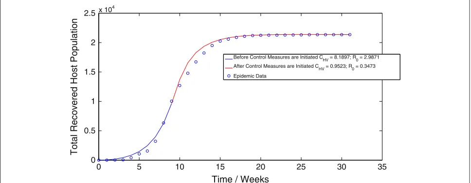
Applying the algorithm for the ordinary least squares (OLS) methodology to the vector-host model (1.1) results in a value ofCHV =8.1897 week−1 before the implemen-tation of control measures and a value ofCHV = 0.9523 week−1 after the implementation of control measures. Thus, we obtain an estimate ofR0 = 2.9871 before the
implementation of control measures and R0 = 0.3473
after the implementation of control measures. The best-fit trajectory of model (1.1) calculated using the OLS methodology, along with the epidemic data is displayed in Figure 1. Similarly, implementing the algorithm for the generalized least squares (GLS) methodology results in a value of CHV = 8.0976 week−1 before the
imple-mentation of control measures and a value of CHV =
1.2374 week−1after the implementation of control mea-sures. Thus, when using the GLS scheme, we obtain
an estimate of R0 = 2.9535 before the
implementa-tion of control measures and R0 = 0.4513 after the
implementation of control measures. Figure 2 displays the best-fit trajectory of model (1.1) calculated using the GLS methodology. We observe that the GLS estimates
for R0 before the implementation of control measures
are in close agreement with the results obtained using the OLS scheme. There is however, difference between the estimates forR0after the implementation of control measures.
Application of the algorithm for the ordinary least squares (OLS) methodology to the direct-transmission
0 5 10 15 20 25 30 35
0 0.5 1 1.5 2 2.5x 10⁴
Time / Weeks
Total Recovered Host Population
Figure 2The best-fit trajectory of model (1.1) calculated using the GLS methodology, along with the epidemic data.
model (3.1) results in a value of β = 3.0302 week−1
before the implementation of control measures and a
value of β = 0.6622 week−1 after the
implementa-tion of control measures. This corresponds to a value
of R0 = 3.0182 before the implementation of control
measures and R0 = 0.6596 after the implementation of
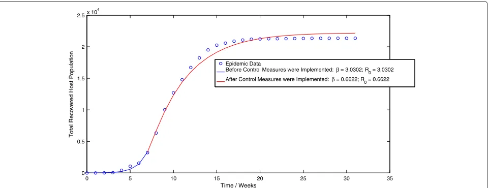
control measures. Figure 3 displays the best-fit trajectory of the direct-transmission model (3.1) calculated using the OLS scheme. We observe that the pre-control value of
R0is slightly larger (1.04%) than the corresponding value obtained by applying the OLS scheme to the vector-host model (1.1), which we feel is not a statistically signifi-cant increase. However, the post-control value of R0 is significantly higher (89.92%) than the corresponding value obtained by applying the OLS scheme to the vector-host model (1.1).
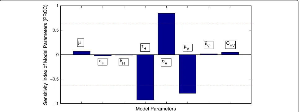
In addition, pre-control estimates ofR0for the dengue epidemic from the uncertainty analysis are shown in Figure 4. The 95% confidence interval for the pre-control value ofR0 is given by(2.0293, 6.5310). The probability thatR0, before the implementation of control measures, is greater than unity is more than 99.9%. Similarly, the sen-sitivity analysis, shown in Figure 5, suggests that the most significant (PRCC values above 0.5 or below−0.5) sensi-tivity parameters toR0areτH,σV andμV. This suggests that these parameters need to be estimated with precision in order to accurately capture the transmission dynamics of dengue.
Furthermore, implementing the algorithm for the gener-alized least squares methodology in the case of the direct-transmission model (3.1) results in a value ofβ = 3.0920 week−1 before the implementation of control measures
Figure 4Uncertainty analysis of the basic reproduction numberR0.
and a value ofβ = 0.5895 week−1 after the implemen-tation of control measures. These values of the contact
rate result in an estimate of R0 = 3.0797 before the
implementation of control measures and R0 = 0.5872
after the implementation of control measures. The best-fit trajectory of the direct-transmission model (3.1) calcu-lated using the GLS scheme is displayed in Figure 6. We observe that while these results are in close agreement with the corresponding results obtained by applying the OLS scheme to the direct-transmission SEIR model, the estimated value of post-controlR0 is again, significantly
larger (30.11%) than the corresponding value obtained by applying the GLS scheme to the vector-host model. How-ever, there is only a slight increase (4.27%) in the estimate for the pre-control value ofR0across the different mod-els, which we again feel is not a statistically significant increase.
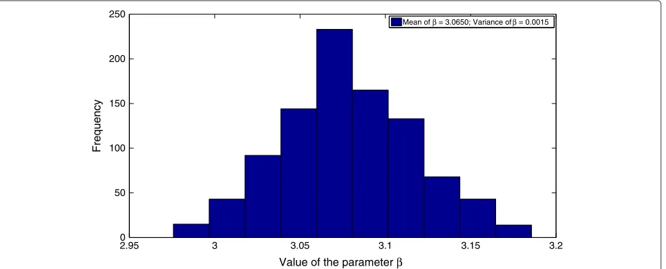
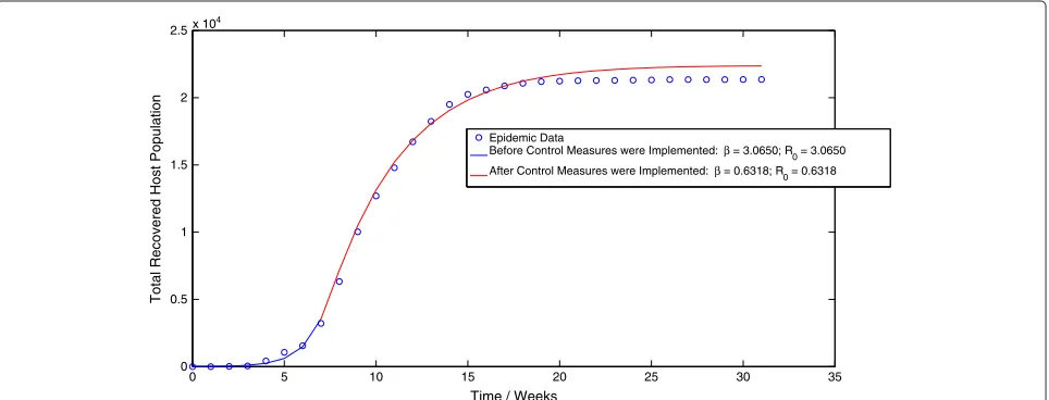
Finally, implementation of the MCMC algorithm to the stochastic direct-transmission model (4.1) results in a value ofβ=3.0650 week−1before the implementation of control measures and a value ofβ = 0.6318 week−1after the implementation of control measures. These values of
Figure 6The best-fit trajectory of model (3.1) calculated using the GLS methodology, along with the epidemic data.
the contact rate correspond to values of R0 = 3.0528
before the implementation of control measures andR0 = 0.6293 after the implementation of control measures. The probability distributions of the contact rateβ, both before and after the implementation of control measures are dis-played in Figure 7 and Figure 8 respectively. Moreover, the mean trajectory of the stochastic model (4.1) calculated using Monte Carlo simulations involving the mean of the posterior distribution is displayed in Figure 9. The results of the MCMC methodology are in close agreement with the results obtained by applying the GLS and OLS schemes to the deterministic direct-transmission model (3.1). Furthermore, there is also close agreement in our estimates for the pre-control value ofR0across both the previous methodologies as well as the different models. There is however, again, a significant difference between
the post-control value ofR0, obtained using the MCMC algorithm and the estimates of the post-control value of
R0, obtained by applying the OLS and GLS scheme to the vector-host model (1.1).
Discussion
We have performed a retrospective analysis of the 2011 dengue fever epidemic in Pakistan and obtained esti-mates of the basic reproduction number R0, from epi-demic data using three different methods.R0, defined as the total number of secondary infections produced by introducing a single infective in a completely susceptible population, is a simple but effective measure of the trans-missibility of an infectious disease. In each case it was observed that the value ofR0was initially well in excess of unity, leading to the observed epidemic outbreak. Some
Figure 8The distribution of the parameterβafter the implementation of control measures.
weeks after the initial outbreak however, control mea-sures were successfully implemented that reduced the value of R0 to less than unity, thus resulting in disease elimination.
Several methods have been proposed for the estima-tion ofR0, both for deterministic as well as for stochastic models. These methods depend upon the mathematical model of the disease as well the nature of the data. In the case of deterministic compartmental models, least squares fit to the data has been widely used to estimate the model parameters [18,30,32]. For stochastic models likeli-hood based techniques have been used by several authors [33,34]. We consider two ODE based deterministic mod-els and a Continuous Time Markov Chain (CTMC) based stochastic model. Using least squares estimation for the
deterministic models and a Markov Chain Monte Carlo based approach for the stochastic model, we compare the value ofR0obtained using the different models. We note that this is the first such study performed for the Dengue Epidemic in Pakistan.
The first inference methodology involved fitting a deter-ministic ODE model for the transmission dynamics of single-strain dengue to the epidemic data using a basic ordinary least squares (OLS) scheme in the context of a statistical model which assumed longitudinally constant variance for the epidemic data. An a priori more realistic methodology was used to fit the deterministic ODE model to obtain estimates of the model parameters using a gen-eralized least squares (GLS) scheme which made use of a statistical model that assumed that variances associated
with the observation process were directly proportional to the measurement values. One of the questions we tried to address was whether or not the variances were strongly dependent on the observations. Finally, we for-mulated a discrete-time, direct transmission, stochas-tic model for the spread of dengue virus and used Markov chain Monte Carlo (MCMC) methods to perform Bayesian inference and estimate the basic reproduction number.
We observe that the estimates for the basic
repro-duction number R0 before the implementation of
con-trol measures are in excellent agreement for the same model across different methodologies. Similarly, across different models there is a very slight but nonetheless statistically insignificant difference in our estimates of the pre-control basic reproduction number. We there-fore conclude that our estimation of the pre-control value of R0 is quite robust, both across different methodolo-gies as well as across different models. This leads us to believe that the noise does not depend significantly on the data. Furthermore, agreement in our estimates across models indicates that both the vector-host model as well as the direct-transmission model can be used to accurately capture the disease dynamics of actual dengue epidemics before the implementation of control measures.
While there is also close agreement in our estimates for the basic reproduction numberR0after the implementa-tion of control measures across different methodologies, there is nonetheless significant difference between the post-control estimates of R0 across the vector-host and direct-transmission models. Specifically, R0 is estimated to be significantly larger in value when using the direct-transmission model as opposed to the vector-host model. We conjecture that this might be due to the fact that the direct-transmission model makes use of an approxi-mation, which involves solving for the equilibrium value of the vector force of infection. Thus, while the vec-tor force of infection rises and peaks for the vecvec-tor-host model, before settling to its equilibrium value, it is in effect equal to the smaller equilibrium value for the direct-transmission model. Therefore, since the vector force of infection for the direct transmission model is, in effect, smaller for the time period after the implementation of control measures, it results in a larger estimate of the basic reproduction number in order to produce a ‘best-fit’ for the observed epidemic data.
Conclusion
In conclusion, we have attempted to assess the transmis-sibility of the dengue virus during the 2011 dengue fever epidemic in Pakistan by estimating the basic reproduc-tion numberR0both before and after the implementation of public health control measures. Our estimates for the
pre-control value ofR0are in close agreement both across different methodologies and the different models. Fur-thermore, the post-control estimates are also in close agreement across the different methodologies. There is however, a significant increase in the estimates of the post-control value ofR0obtained using the direct-transmission model compared to estimates obtained using the vector-host model.
Methods
Methods and materials for statistical inference using the vector-host model
The vector-host epidemic Model
The model is a deterministic vector-host ODE model that assumes a homogeneous mixing of the host (human) and vector (mosquito) populations. The total human popula-tion at timet, denoted byN(t), is divided into four mutu-ally exclusive classes comprising of susceptible humans
SH(t), exposed humansEH(t), infected humansIH(t)and recovered humans RH(t). It is assumed that individuals who recover from infection with a particular serotype of Dengue gain lifelong immunity to it [2]. Similarly, the total vector population at time t is denoted by NV(t) and is divided into three mutually exclusive classes com-prising susceptible of susceptible vectorsSV(t), exposed vectors EV(t) and infected vectors IV(t). It is assumed that vectors (mosquitoes) infected with a particular serotype of Dengue never recover [2]. We also modify the original model of Garba et al. [11] by assuming that exposed humans and exposed vectors do not transmit the disease.
The model assumes that the susceptible human pop-ulation SH(t) has a constant recruitment rate H and natural death rateμ. Susceptible individuals are infected with Dengue virus (due to contact with infected vectors) at a rate λH and thus enter the exposed class EH. The exposed populationEH(t)is depleted at the natural death rateμ. Additionally, exposed individuals develop symp-toms and move into the infected class IH at a rate σH. The infected populationIH(t)is depleted via the natural death rateμ, the disease-induced death rateδH and the recovery rate of infected individualsτH. Finally, the recov-ered populationRH(t)decreases due to the natural death rateμ.
Mathematically, the model is a follows
dSH
dt =H−λHSH−μS dEH
dt =λHS−(σH+μ)EH dIH
dt =σHEH−(τH +μ+δH)IH dRH
dt =τHIH−μRH dSV
dt =V −λVSV−μVSV dEV
dt =λVSV −(σV +μV)EV dIV
dt =σVEV −(μV +δV)IV
where,
λH=CHV
IV
NH
λV =CHV
IH
NH
(1.1)
A description of the variables and parameters of the model (1.1) is given in Table 1.
Garba et al. [11] have calculated the basic reproduction number R0 for their original model. Although, we have made a slight modification to the original model, the basic reproduction number for our model is not significantly different. Hence, for the model (1.1),R0is given by
R0=
C2HVVμσHσV HμVk1k2k3k4
(1.2)
where
k1=σH+μH k2=τH+μH+δH
k3=σV +μV and k4=μV+δV
Table 1 Description of the variables of the vector-host model (1.1)
Variable Description
NH(t) Total host population
SH(t) Population of susceptible hosts
EH(t) Population of exposed hosts
IH(t) Population of infected hosts
RH(t) Population of recovered hosts
NV(t) Total vector population
SV(t) Population of susceptible vectors
EV(t) Population of exposed vectors
IV(t) Population of infected vectors
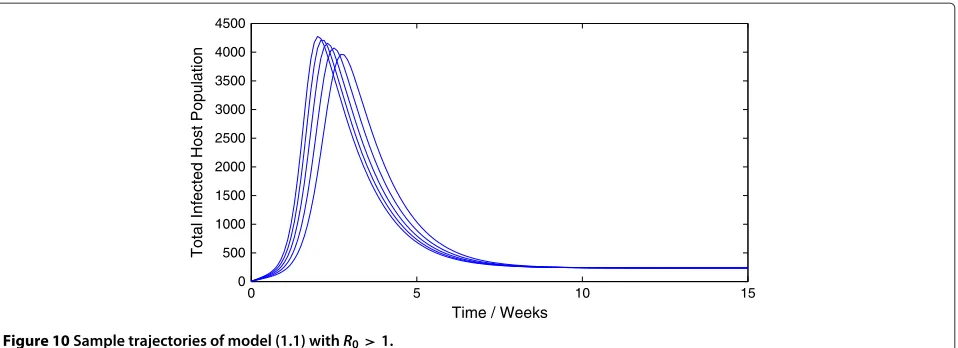
Representative trajectories of the model (1.1) for differ-ent values ofR0are given in Figure 10 and Figure 11. As expected, a value ofR0greater than unity leads to an epi-demic while a value ofR0 less than unity leads to swift disease elimination.
Data sources
The epidemic data used in this study was collected by the Punjab Disaster Management Authority (PDMA) dur-ing the 2011 Dengue Epidemic in Punjab, Pakistan. The data, displayed in Figure 12, represents the cumulative number of dengue fever cases reported over a 32-week period extending from the 1stof August 2011, to the 20th of February 2012. The data was collected from a number of public and private hospitals in the major metropoli-tan centers of Punjab, including Lahore, Faisalabad and Multan. Patients were classified as infected with dengue virus based on the results of laboratory tests for the dengue specific antibodies Immunoglobulin G (IgG) and Immunoglobulin M (IgM). As per the Government of Pak-istan’s directives, the laboratory test was available at a subsidized rate in all major hospitals in the capital city of Lahore. It is therefore unlikely that poverty played a serious role in under-reporting of dengue fever cases.
Prior to August 2011, there were three reported cases of dengue fever, all occurring several months before the actual epidemic. This leads us to conclude that these were isolated incidents and were not directly related to the epidemic itself. Furthermore, nearly 87% of all dengue infections were caused by a single serotype (DEN2) of the dengue virus. This justifies our use of a single-strain epidemic model as opposed to dengue models that incor-porate the effects of cross-immunity and ADE.
Estimation schemes
In order to calculateR0, we require the values of several parameters used in model (1.1). Furthermore, we require knowledge of the initial conditions that will be used to simulate trajectories of the model (1.1).
Estimates for several of the model parameters used in model (1.1) can be obtained from existing studies on Dengue Fever. Table 2 lists these parameters along with reasonable estimates of their values.
The recruitment rate for the susceptible host population depends on the demographics of the urban population that is being considered. This study uses epidemic data collected during the 2011 Dengue Epidemic in Punjab, Pakistan. Therefore, in the absence of concrete estimates, the host recruitment rate has been chosen so as to allow for a realistic steady state host population.
0 5 10 15 0
500 1000 1500 2000 2500 3000 3500 4000 4500
Time / Weeks
Total Infected Host Population
Figure 10Sample trajectories of model (1.1) withR0>1.
directly. Most previous studies have used assumed values for the effective contact rate [11-13]. Thus, it is not pos-sible to directly estimate the basic reproduction number. Consequently, we will adopt an indirect approach, similar to previous studies such as [30] and [18], by first finding the value of the parameterCHV for which the model (1.1) has the best agreement with the epidemic data, and then using the resultant parameter values to estimateR0.
As mentioned before, for the purpose of simulating model (1.1) we require knowledge of the initial con-ditions. It is possible to consider the initial conditions (SH(0),EH(0),IH(0),RH(0),SV(0),EV(0),IV(0))as model
parameters along with the effective contact rate CHV
and estimate values for all parameters. Such a tech-nique, however, produces slightly unreliable results. This is explained by the fact that the available epidemic data is restricted to the cumulative number of dengue cases reported, while the optimization schemes that we will employ produces estimates for eight variables. There are thus too many degrees of freedom and the ‘best-fit’ may result in unrealistic estimates for the initial conditions.
We will therefore use reasonable estimates for the initial conditions and restrict ourselves to optimizing only the effective contact rateCHV.
Table 3 displays the initial conditions that were therefore chosen.
In the following sections we will employ different methods to estimate the parameterω=CHVby minimiz-ing the difference between the predictions of model (1.1) and the epidemic data.
Ordinary Least Squares Estimation
We will first attempt to estimate the effective contact rate by fitting the best trajectory of model (1.1) to the epi-demic data using an ordinary least squares (OLS) scheme, implemented using thefminsearch function in the built-in Optimization Toolbox built-in MATLAB. This will allow us to estimate the parameterωand thus calculate the basic reproduction numberR0.
In order to fit model trajectories with the observed epidemic data, we will assume that all reported cases recovered from the infection after a time lag of two weeks.
0 2 4 6 8 10 12 14 16 18 20
0 10 20 30 40 50 60 70
Time / Weeks
Total Infected Host Population
0 5 10 15 20 25 30 0
0.5 1 1.5 2 2.5x 10
4
TIme / Weeks
Cumulative Reported Cases of Dengue Fever
Figure 12The cumulative number of dengue cases during the 2011 dengue fever epidemic in Pakistan as reported by the Punjab Disaster Management Authority (PDMA).
Thus, the epidemic data, after a lapse of two weeks, rep-resents the total recovered host population. In addition, in order to account for the effect of control measures that were implemented during the actual epidemic, we have assumed that the transmission rateCHV is a function of time t. We will assume that the transmission rate was constant up until the point when control measures were implemented, whereupon it changed to a different con-stant value. An alternative definition of the contact rate is also given in [33]. Thus, mathematically,
CHV(t)=
CHV1 t<t∗
CHV2 t≥t∗
(2.1)
wheret∗is the time at which control measures were first implemented. For the purpose of this study and in view of
Table 2 Description of the parameters of the vector-host model (1.1)
Parameter Description Value Reference
H Host recruitment rate 140 week−1 assumed
V Vector recruitment rate 28000 week−1 [12] 1
μ Host mortality 3494 weeks [12]
δH Host disease-induced death rate
0.0035 week−1 [12]
1 μV
Vector mortality 2 weeks [12]
δV Vector disease-induced death rate
negligible week−1 [11]
1 σH
Latency period for exposed hosts
1 week [13]
1 τH
Recovery time for infected hosts
1 week [12]
1 σV
Latency period for exposed vectors
10
7 weeks [13]
CHV Effective contact rate Variable
no concrete information being available in this regard, we have assumed thatt∗=8 weeks.
For the purpose of this section we shall employ the nota-tion and methodology developed in [30]. Essentially, we will employ inverse problem methodology to obtain esti-mates ofω=CHV by minimizing the difference between the observed weekly cumulative number of recovered host individuals and the model predictions using a ordinary least squares (OLS) criterion. This will be done in the context of an appropriate statistical model.
The ordinary least squares estimation methodology that we will employ is based on model (1.1) as well as an appro-priate statistical model for the observation process. Thus, similar to [30], we assume that the model (1.1), together with a ‘true’ value of the parameterω, given byω0, per-fectly describes the transmission dynamics of the dengue epidemic. Moreover, we assume that theN observations,
Yj, given by the epidemic data, are generated by a statis-tical process. However, the N observations also contain random deviations from the underlying statistical process. Hence, following [30], it is assumed that
Yj=p(tj,ω0)+ j forj=1, 2, 3,. . .,N (2.2)
Table 3 Initial conditions used when applying the OLS and GLS methodology to the vector-host model (1.1)
Initial condition Value
SH(0) 1 million
EH(0) 15
IH(0) 3
RH(0) 0
SV(0) 0.1 million
EV(0) 60
where p(tj,ω0) denotes wherep(tj,ω0) denotes the total number of infected individuals who recover in the time span of weekjwhen using the ‘true’ parameterω0. Thus, it is assumed that the observed epidemic data is a partic-ular realization of the statistical model (2.2). Under the framework of model (1.1) therefore,
p(tj,ω0)=
tj
tj−1
τHIH(t,ω0) forj=1, 2, 3,. . .,N
(2.3)
wheret0denotes the time of start of the statistical process and the time of each observation is given by and ordered ast0<t1<t2. . .. .<tN.
The error terms j, are assumed to be independent,
identically distributed (i.i.d) random variables, each with zero mean and finite variance. No further assumptions are made regarding the distribution of j. In particular, it is not assumed that the distribution is normal. Thus,E[ j]= 0 andvar( j) = σ2. Note that, the i.i.d assumption implies that the variance for each error term j is identical. We therefore have
EYj
=p(tj,ω0)andvar(Yj)=σ2forj=1, 2, 3,. . .,N For a set of observations{Yj}Nj=1, produced by the statis-tical model (2.2), we define the statisstatis-tical estimatorωOLS as
ωOLS(Y)=arg min ω∈
j=N
j=1
[Yj−p(tj,ω)]2. (2.4)
where ⊂ Ris defined as the physically and biologi-cally feasible region for the parameterω. In other words, the statistical estimator is the solution of the following equations
j=N
j=1
[Yj−p(tj,ω)] ∂
∂ωp(tj,ω)=0. (2.5)
It is clear that the statistical estimator ωOLS is a ran-dom variable since each error term jis a random variable. Furthermore, the estimator attempts to minimize the dis-tance between the observed weekly cumulative number of recovered host individuals and the predictions of model (1.1). A subsequent detailed description of how to obtain the probability distribution associated withωOLSis given in [30]. Our goal in the current study will be to obtain the mean of the probability distribution ofωOLS.
Uncertainty and sensitivity analysis ofR0
As mentioned previously, the basic reproduction
num-ber R0 for the deterministic model (1.1) is given by
(1.2) Thus, the value of R0 depends on the variables
CHV,H,μ,σH,δH,τH,V,σV,μV andδV. While deter-ministic models implicitly assume that the model parame-ters are not stochastic in nature, an element of uncertainty
is always associated with estimates of these parameters due to factors such as natural variation, errors in mea-surements and lack of measuring techniques. In general, uncertainty analysis quantifies the degree of confidence in the parameter estimates by producing 95% confidence intervals (CI) which can be interpreted as intervals con-taining 95% of future estimates when the same assump-tions are made and the only noise source is observation error. Additionally, sensitivity analysis identifies critical model parameters and quantifies the impact of each input parameter on the value of an output. In this section, we shall perform uncertainty and sensitivity analysis of the basic reproduction number R0. A detailed descrip-tion of the history and methodology of uncertainty and sensitivity analysis is given in [35].
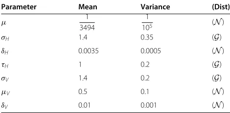
We will use Latin hypercube sampling (LHS) [35] to quantify the uncertainty in and sensitivity ofR0as a func-tion of the 7 model parameters (CHV,μ,σH,δH,τH,σV,μV and δV). It is assumed, following [33], that the recruit-ment ratesV andH are constants. This will enable us to obtain CI for the value of R0that we have estimated in the last section. For the sensitivity analysis, the partial rank correlation coefficient (PRCC) technique [35] will be used to assess the impact of changes in parameter values on the value ofR0. PRCC, which uses rank transformation of the data to reduce the effects of non-linearity, provides a measure of monotonicity after the removal of the linear effects of all but one model parameter. PRCC is therefore a global sensitivity analysis technique. The assumed distri-butions of the model parameters used in the two analyses are mentioned in Table 4.
Generalized least squares estimation
The Ordinary Least Squares Estimation (OLS) scheme we employed in the previous section assumed that the variances associated with the epidemic observations were longitudinally constant and not dependent on the values of the observations. This may not be a realistic assumption especially if the epidemic data is influenced by a source
Table 4 Assumed probability distributions for the parameters of the model (1.1) used in the sensitivity and uncertainty analysis
Parameter Mean Variance (Dist)
μ 1
3494
1
105 (N)
σH 1.4 0.35 (G)
δH 0.0035 0.0005 (N)
τH 1 0.2 (G)
σV 1.4 0.2 (G)
μV 0.5 0.1 (N)
of non-constant systematic error such as under-reporting. Indeed, under-reporting of dengue cases has been well documented in previous studies such as [36] and [37].
If indeed the epidemic data that is being used in the current study is influenced by under-reporting then the assumption of constant variances associated with the observations is not correct since observation errors will now be proportional to the size of the mea-surement. Hence, we must use a statistical model, which assumes longitudinally non-constant and model depen-dent variances for the epidemic observations. In this section therefore, we will attempt to estimate the effective contact rate by fitting the best trajectory of model (1.1) to the epidemic data using a generalized least squares (GLS) scheme. An excellent discussion on the use of the OLS and GLS scheme and different statistical models depend-ing on the assumptions regarddepend-ing the error present in the observation process is given in [38].
Once again we shall employ the notation and method-ology developed in [30]. Apart from the assumptions of the statistical model, as before, we will assume that all reported cases recovered from the infection after a time lag of two weeks and that therefore, the epidemic data, after a lapse of two weeks, represents the total recovered host population. Furthermore, we will again assume that the effective contact rateCHV is a function of time. Thus, mathematically, Eq. 2.1 wheret∗is the time at which con-trol measures were first implemented. As before, we have assumed thatt∗=8 weeks.
Again, following [30], we will employ inverse problem methodology to obtain estimates ofω=CHVby minimiz-ing the difference between the observed weekly cumula-tive number of recovered host individuals and the model predictions using a generalized least squares (GLS) crite-rion. This will be done in the context of a statistical model, which assumes that the error in the observation process is directly proportional to the values of the measurement. Hence, it is assumed that
Yj=p(tj,ω0)+p(tj,ω0) j forj=1, 2, 3,. . .,N (2.6)
where denotes wherep(tj,ω0)denotes the total number of infected individuals who recover in the time span of week
jusing the ‘true’ parameterω0. Thus, it is assumed that the observed epidemic data is a particular realization of the statistical model (4.1). Under the framework of model (1.1) therefore,
p(tj,ω0)=
tj
tj−1
τHIH(t,ω0) forj=1, 2, 3,. . .,N
(2.7)
wheret0denotes the time of start of the statistical process and the time of each observation is given by and ordered ast0<t1<t2. . .. .<tN.
The rest of the analysis is similar to the method outlined in the previous section and follows easily.
Methods and materials for statistical inference using the direct-transmission model
The direct transmission epidemic model
Several existing studies on the transmission dynamics of dengue use a direct transmission SEIR model [13]. The direct transmission models can be obtained using an approximation to vector-host models such as model (1.1). First, it is assumed that the vector force of infec-tion can be approximated by solving for the equilibrium values of the vector population compartments. Further-more, it is assumed that the susceptible vector popula-tion is approximately a linear multiple of the total host population. These two assumptions effectively result in a rescaling of the host effective contact rate CHV of model (1.1) into a direct transmission contact parame-terβ. Using the aforementioned approximation, we for-mulate a standard incidence, direct transmission SEIR model. More details of the approximation are given in [13].
Mathematically, the direct-transmission model is a follows
dS(t)
dt = −
βS(t)I(t)
N(t) −μS(t)
dE(t)
dt =
βS(t)I(t)
N(t) −(σ+μ)E(t)
dI(t)
dt =σE(t)−(τ+μ+δ)I(t) dR(t)
dt =τI(t)−μR(t)
(3.1)
where
N(t)=S(t)+E(t)+I(t)+R(t)
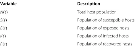
A description of the variables and parameters of the model (3.1) is given in Table 5 and Table 6 respectively.
For the direct transmission model (3.1), the basic
repro-duction number R0 is defined as the total number of
secondary infections produced by introducing a single infected host in a completely susceptible population.
Table 5 Description of the variables of the direct-transmission model (3.1)
Variable Description
N(t) Total host population
S(t) Population of susceptible hosts
E(t) Population of exposed hosts
I(t) Population of infected hosts
Table 6 Description of the parameters of the direct-transmission model (3.1)
Parameter Description 1
μ Host mortality
δ Host disease-induced death rate 1
σ Latency period for exposed hosts 1
τ Recovery time for infected hosts
β Effective contact rate for the direct transmission model
Therefore, for model (3.1), the basic reproduction number
R0is given by:
R0=
βσ
(τ+δ+μ)(σ+μ)
As discussed previously, the existing literature on dengue fever provides excellent estimates of all the param-eters of Model (3.1) with the exception of the contact rate β. Hence, our aim will be to estimate the contact rate β using statistical inference and thereby estimate the basic reproduction numberR0. The basic methodology used for both the OLS and GLS schemes will be similar to the process outlined in the previous sections.
In order to account for the effect of control measures that were implemented during the actual epidemic, we have assumed that the contact rate β(t)is a function of timet. We will assume that the contact rate was constant up until the point when control measures were imple-mented, whereupon it changed to a different constant value. Hence, mathematically,
β(t)=
β1 t<t∗
β2 t≥t∗
(3.2)
wheret∗is the time at which control measures were first implemented. For the purpose of this study and in view of no concrete information being available in this regard,
we have assumed that t∗ = 6 weeks. We observe that
β(t)is most likely not a continuous function of timet. An alternative definition of the transmission rate β(t), as a continuous function of time, is given in [33].
The stochastic model and Markov Chain Monte Carlo (MCMC)
In this section we formulate a stochastic, direct-transmission, discrete-time, (S)usceptible, (E)xposed, (I)nfected and (R)ecovered/(R)emoved (SEIR) model for the transmission dynamics of dengue virus. We then use standard Markov chain Monte Carlo (MCMC) methods to perform Bayesian Inference on the epidemic data to obtain estimates of the basic reproduction number R0. As mentioned in [13], a number of studies exist on the transmission dynamics of dengue that assume direct-transmission. Moreover, a simple approximation can be
used to reduce a vector-host model for dengue virus to a direct transmission model (see [13] and the references given therein for more details). The purpose of using a direct-transmission model is to make stochastic inference computationally tractable. For the purpose of this study, we will broadly follow the procedure outlined in [33].
Stochastic model formulation
The stochastic SEIR model we will consider is a discrete-time model that has been formulated and discussed pre-viously in [25,33]. LetS(t),E(t),I(t)andR(t)denote the susceptible host, exposed host, infected host and removed or recovered host populations at time t respectively. As is common, our model will assume homogenous mixing of all individuals. Furthermore, consider a time interval (t,t+ h], where h denotes the length of time between two observations of the epidemic. In this case therefore,
his one week. Now, letB(t) denote the number of sus-ceptible individuals who have contracted disease,C(t)the number of exposed individuals who have become infected andD(t)the number of infected individuals who die or have recovered from the disease during this time inter-val. For the sake of simplicity, and keeping in view the low mortality rate associated with dengue fever, we will assume that the disease-induced death rate is negligible. Following [33], and in view of the fact that the dynam-ics of dengue disease take place on a much smaller time scale than the average human life expectancy, we will
assume that the total population N remains constant.
Thus, mathematically the stochastic model is given by
S(t+h)=S(t)−B(t)
E(t+h)=E(t)+B(t)−C(t)
I(t+h)=I(t)+C(t)−D(t)
S(t)+E(t)+I(t)+R(t)=N
(4.1)
where,
B(t)∼Bin(S(t),λ(t)), C(t)∼Bin(E(t),kσ) and B(t)∼Bin(I(t),kτ)
are random variables with binomial distributions. The probability of success for these binomial random variables is given by
λ(t)=1−exp
β(t)I(t)
N h
kσ =1−exp(−σh) kτ =1−exp(−τh)
(4.2)
Here,β(t),1 σ and
1
probability that each individual will stay in a specific com-partment for a time periodhis given byexp(h), where is the compartment specific movement rate. The binomial distributions in (4.2) are then obtained by summing over the individual Bernoulli trials for every individual in the compartment. It is assumed that each trial is independent and identical for every member of the compartment.
Similar to the previous section, we will assume that the contact rate β(t) is a function of time t. Thus, mathe-matically, Eq. (3.2) wheret∗ is the time at which control measures were first implemented. As before, we have assumed thatt∗=8 weeks.
The stochastic model (4.1) makes use of the parame-tersβ(t),σandτ. Of these parameters, estimates ofσand τ can be obtained from existing studies on dengue virus and have been given previously. Therefore, our aim will be to estimate the parameterβ(t)using the epidemic data and estimates of initial population sizes. For this purpose, we define the parameter vector, which we will attempt to estimate, as=β(t). Moreover, we define
B= {B(t)}tt==τ0∗
C= {C(t)}tt==τ0∗
D= {D(t)}tt==τ0∗
(4.3)
whereτ∗ denotes the time at which observations of the epidemic have finished.
Thus, based on the available epidemic data, we have complete knowledge of bothCandDbut no knowledge of B. This lack of knowledge will be a major cause of uncer-tainty in our analysis. Nevertheless, we will attempt to estimateR0for both the time period before control mea-sures are implemented and the time period after control measures are implemented using our knowledge of both CandD.
Inference methodology
Based on the definitions given in (4.1) and (4.2), we observe thatB(t),C(t) and D(t) are conditionally inde-pendent random variables. Thus, the likelihood function for the data set{B,C,D}is given by
L(B,C,D|)= t=τ∗
t=0
f1(B(t)|.)f2(C(t)|.)f3(D(t)|.) (4.4)
wheref1,f2 andf3are the binomial transition probabili-ties given in (4.1) and (4.2), conditioned onand all the epidemic data represented byB, C andDup until time
t. Therefore, the maximum likelihood estimator for the parameter vector, and by extension forβ(t)andR0can be obtained by maximizing the expression in (4.4).
According to model (4.1), the time series for
S(t),E(t),I(t) andR(t) can be obtained using B(t),C(t) andD(t). Unfortunately as mentioned previously,B(t)is unknown since the process of infection is not observed.
Hence, we must also impute the values of B(t). These values can then be used to construct the time series for
S(t)andE(t).
Since, the likelihood function forB,CandD, denoted as
L(B,C,D|), is given by (4.4), we can use Bayes’ Theorem to obtain, up to a constant, the required posterior dis-tribution that we wish to sample from. This is given by
L(,B|C,D)∝L(B,C,D|)π() (4.5)
whereπ()is the prior distribution. Thus, our MCMC
algorithm will sample from the conditional probability distributions π(|B,C,D) andπ(B|,C,D) to produce samples from the required distribution π(,B|C,D). In short, our general algorithm will proceed as follows
• Initialize the setBusing any appropriate initial vector.
• Since,CandDare known, construct the time series forS(t),E(t),I(t)andR(t).
• Initialize the parameter vector.
• UpdateBusing the conditional distribution π(B|,C,D).
• Reconstruct the new time series forS(t),E(t),I(t) andR(t).
• Updateusing the conditional distribution π(|B,C,D).
• Repeat steps4−6until the Markov chain has converged and subsequently, the required samples have been obtained.
To sample fromπ(B|,C,D) one can use the condi-tional binomial distribution forB, making sure that the choice is consistent with the final size and length of the epidemic. This is however computationally very ineffi-cient as most of the draws would be rejected due to the consistency condition. To avoid this issue we condition the proposal on the observed extinction time, following the method described in [33] for computationally efficient sampling.π(|B,C,D) is updated using a random walk proposal.
Inference from the observed dengue data
An important question that arises at this point pertains to the meaning and significance of the basic reproduction
Table 7 Posterior mean of the contact rate and basic reproduction number for the Stochastic
direct-transmission model (4.1)
Parameter Posterior mean
β1 3.0650 week−1
β2 0.6318 week−1
R0before control measures 3.0528
numberR0for the stochastic SEIR model. As mentioned previously and as discussed in detail in [31], the basic reproduction numberR0for the deterministic SEIR model is essentially a threshold quantity which determines the possibility of an outbreak of the disease. Thus, for the deterministic SEIR model, ifR0is less than unity there is no epidemic while ifR0is greater than unity there will be a disease epidemic.
Unfortunately, the threshold dynamics of the stochas-tic SEIR model are not the same. It can be proven that in contrast to the deterministic model, the stochastic SEIR model predicts disease extinction regardless of the value ofR0. This results in difficulty regarding the interpreta-tion ofR0as a threshold quantity. Therefore, it is tempting to ask the question: what is the importance ofR0in the stochastic SEIR model? An answer to this question may be conjectured (but not proven) by referring to [39]. It is proven in [39] that for the stochastic SI model, on average no epidemic will occur ifR0 < 1, while forR0 > 1 there is a finite probability that an endemic quasi-equilibrium will develop. We conjecture that this result also holds true for the stochastic SEIR model and that it can therefore be used to explain the significance of R0 as a threshold quantity for the stochastic SEIR model.
Using the MCMC algorithm discussed in the previ-ous section, we estimate the transmission rateβ(t) and hence the basic reproduction number R0, both for the time period before control measures are implemented and the time period after the control measures are
imple-mented. We have taken t∗ = 8 weeks and the initial
population sizes to be the same as in the case of infer-ence from the deterministic model using the GLS and OLS schemes. Furthermore, we have taken an uniform prior distribution for the parameter vector. We observe that the results of the MCMC algorithm, displayed in Table 7, are in close agreement with the corresponding results obtained from application of the OLS and GLS schemes to the direct-transmission deterministic model.
Additional file
Additional file 1: Multilingual abstracts in the six official working languages of the United Nations.
Competing interests
The authors declare that they have no competing interests.
Authors’ contributions
MI and AK gave initial input and directed the research. MH implemented the algorithms, carried out the programming and drafted the manuscript. AK interpreted the results and edited the manuscript. All authors read and approved the final manuscript.
Acknowledgements
The authors would like to acknowledge and thank the Punjab Disaster Management Authority for providing the data used for the research work being presented in this article.
Author details
1Department of Mathematics, Lahore University of Management Sciences,
DHA, Lahore, Pakistan.2Department of Mathematics, Swiss Federal Institute of
Technology (ETH), Zurich, Rämistrasse 101, 8092 Zurich, Switzerland.
Received: 26 September 2013 Accepted: 6 March 2014 Published: 7 April 2014
References
1. Ranjit S, Kissoon N:Dengue hemorrhagic fever and shock syndromes. Pediatr Crit Care Med2011,12:90–100.
2. World Health Organization: dengue and severe dengue fact sheet.
2012. [http://www.who.int/mediacentre/factsheets/fs117/en/] 3. Gubler DJ:Dengue and dengue hemorrhagic fever.Clin Microbiol Rev
1998,11(3):480–496.
4. Halstead S, Nimmannitya S, Cohen S:Observations related to pathogenesis of dengue hemorrhagic fever. IV. Relation of disease
severity to antibody response and virus recovered.Yale J Biol Med
1970,42(5):311–322.
5. Kautner I, Robinson MJ, Kuhnle U:Dengue virus infection:
epidemiology, pathogenesis, clinical presentation, diagnosis, and
prevention.J Pediatr1997,131(4):516–524.
6. Shekhar C:Deadly dengue: new vaccines promise to tackle this
escalating global menace.Chem Biol2007,14(8):871–872.
7. Holmes EC, Twiddy SS:The origin, emergence and evolutionary
genetics of dengue virus.Infect Genet Evol2003,3:19–28.
8. Whitehorn J, Farrar J:Dengue.Br Med Bull2010,95:161–173. 9. Gubler D, Kuno G:Dengue and Dengue Hemorrhagic Fever. London: CAB
INTERNATIONAL; 1997.
10. Kawaguchi I, Sasaki A, Boots M:Why are dengue virus serotypes so distantly related? Enhancement and limiting serotype similarity
between dengue virus strains.Proc R Soc Lond B Biol Sci2003,
270(1530):2241–2247.
11. Garba SM, Gumel AB:Abu Bakar MR: Backward bifurcations in
dengue transmission dynamics.Math Biosci2008,215:11–25.
12. Garba S, Gumel A:Effect of cross-immunity on the transmission
dynamics of two strains of dengue.Int J Comput Math2010,
87(10):2361–2384.
13. Wearing HJ, Rohani P:Ecological and immunological determinants of
dengue epidemics.Proc Natl Acad Sci2006,103(31):11802–11807.
14. Esteva L, Vargas C:Coexistence of different serotypes of dengue
virus.J Math Biol2003,46:31–47.
15. Ferguson N, Anderson R, Gupta S:The effect of antibody-dependent enhancement on the transmission dynamics and persistence of
multiple-strain pathogens.Proc Natl Acad Sci1999,96(2):790–794.
16. Esteva L, Vargas C:A model for dengue disease with variable human
population.J Math Biol1999,38(3):220–240.
17. Esteva L, Vargas C:Analysis of a dengue disease transmission model. Math Biosci1998,150(2):131–151.
18. Chowell G, Diaz-Dueñas P, Miller J, Alcazar-Velazco A, Hyman J, Fenimore P, Castillo-Chavez C:Estimation of the reproduction number
of dengue fever from spatial epidemic data.Math Biosci2007,
208(2):571–589.
19. Allen LJ:An introduction to stochastic epidemicmodels.In
Mathematical Epidemiology, Volume 1945 of Lecture Notes in Mathematics. Edited by Brauer F, Driessche P, Wu J. Springer Berlin Heidelberg, 14197 Berlin Germany; 2008:81–130.
20. Keeling MJ, Ross JV:On methods for studying stochastic disease
dynamics.J R Soc Interface2008,5(19):171–181.
21. Bailey NT:A simple stochastic epidemic.Biometrika1950,37:193–202. 22. Allen LJ, Flores DA, Ratnayake RK, Herbold JR:Discrete-time
deterministic and stochastic models for the spread of rabies.
Appl Math Comput2002,132(2):271–292.
23. Weiss GH, Dishon M:On the asymptotic behavior of the stochastic and
deterministic models of an epidemic.Math Biosci1971,11(3):261–265.
24. Tuite AR, Tien J, Eisenberg M, Earn DJ, Ma J, Fisman DN:Cholera epidemic in Haiti, 2010: using a transmission model to explain spatial spread of disease and identify optimal control interventions. Ann Intern Med2011,154(9):593–601.
25. Allen L, Driessche P:Stochastic epidemic models with a backward
26. de Souza DR, Tomé T, Pinho ST, Barreto FR, de Oliveira MJ:Stochastic
dynamics of dengue epidemics.Phys Rev E2013,87:012709.
27. Spencer S:Stochastic epidemic models for emerging diseases. PhD thesis: University of Nottingham; 2008.
28. Allen LJ:An Introduction to Stochastic Processes with Applications to Biology. New Jersey: Pearson Education; 2003.
29. Allen LJ, Burgin AM:Comparison of deterministic and stochastic SIS
and SIR models in discrete time.Math Biosci2000,163:1–33.
30. Cintrón-Arias A, Castillo-Chávez C, Bettencourt LM, Lloyd AL, Banks H:
The estimation of the effective reproductive number from disease
outbreak data.Math Biosci Eng2009,6(2):261–282.
31. Van den Driessche P, Watmough J:Reproduction numbers and sub-threshold endemic equilibria for compartmental models of
disease transmission.Math Biosci2002,180:29–48.
32. Chowell G, Hengartner N, Castillo-Chavez C, Fenimore F, Hyman J:
The basic reproductive number of Ebola and effects of public health
measures: the cases of Congo and Uganda.J Theor Biol2004,
229:119–126.
33. Lekone PE, Finkenstädt BF:Statistical inference in a stochastic epidemic SEIR model with control intervention: Ebola as a case
study.Biometrics2006,62(4):1170–1177.
34. O’Neill P, Roberts GO:Bayesian inference for partially observed
stochastic epidemics.J R Statisitcal Soc A1999,162:121–129.
35. Sanchez MA, Blower SM:Uncertainty and sensitivity analysis of the
basic reproductive rate: tuberculosis as an example.Am J Epidemiol
1997,145(12):1127–1137.
36. Suaya JA, Shepard DS, Beatty ME:Dengue: burden of disease and costs
of illness.InTDR. Report of the Scientific Working Group Meeting on
Dengue. Geneva Switzerland: World Health Organization; 2006:35–49. 37. Beatty ME, Beutels P, Meltzer MI, Shepard DS, Hombach J, Hutubessy R,
Dessis D, Coudeville L, Dervaux B, Wichmann O, Margolis HS, Kuritsky JN:
Health economics of dengue: a systematic literature review and
expert panel’s assessment.Am J Trop Med Hyg2011,84(3):473–488.
38. Banks HT, Davidian M, Jr Samuels JR, Sutton KL:An Inverse Problem Statistical Methodology Summary: 3994 AK Houten Netherland; 2009. 39. Jacquez JA, O’Neill P:Reproduction numbers and thresholds in
stochastic epidemic models I. Homogeneous populations. Math Biosci1991,107(2):161–186.
doi:10.1186/2049-9957-3-12
Cite this article as:Khanet al.:Estimating the basic reproduction number
for single-strain dengue fever epidemics. Infectious Diseases of Poverty
20143:12.
Submit your next manuscript to BioMed Central and take full advantage of:
• Convenient online submission
• Thorough peer review
• No space constraints or color figure charges
• Immediate publication on acceptance
• Inclusion in PubMed, CAS, Scopus and Google Scholar
• Research which is freely available for redistribution