RESEARCH ARTICLE
Natural speciation of nickel
at the micrometer scale in serpentine
(ultramafic) topsoils using microfocused X-ray
fluorescence, diffraction, and absorption
Matthew G. Siebecker
1,2*, Rufus L. Chaney
3and Donald L. Sparks
1,2Abstract
Serpentine soils and ultramafic laterites develop over ultramafic bedrock and are important geological materials from environmental, geochemical, and industrial standpoints. They have naturally elevated concentrations of trace metals, such as Ni, Cr, and Co, and also high levels of Fe and Mg. Minerals host these trace metals and influence metal mobil-ity. Ni in particular is an important trace metal in these soils, and the objective of this research was to use microscale (µ) techniques to identify naturally occurring minerals that contain Ni and Ni correlations with other trace metals, such as Fe, Mn, and Cr. Synchrotron based µ-XRF, µ-XRD, and µ-XAS were used. Ni was often located in the octahedral layer of serpentine minerals, such as lizardite, and in other layered phyllosilicate minerals with similar octahedral struc-ture, such as chlorite group minerals including clinochlore and chamosite. Ni was also present in goethite, hematite, magnetite, and ferrihydrite. Goethite was present with lizardite and antigorite on the micrometer scale. Lizardite integrated both Ni and Mn simultaneously in its octahedral layer. Enstatite, pargasite, chamosite, phlogopite, and for-sterite incorporated various amounts of Ni and Fe over the micrometer spatial scale. Ni content increased six to seven times within the same 500 µm µ-XRD transect on chamosite and phlogopite. Data are shown down to an 8 µm spatial scale. Ni was not associated with chromite or zincochromite particles. Ni often correlated with Fe and Mn, and gener-ally did not correlate with Cr, Zn, Ca, or K in µ-XRF maps. A split shoulder feature in the µ-XAS data at 8400 eV (3.7 Å−1 in k-space) is highly correlated (94% of averaged LCF results) to Ni located in the octahedral sheet of layered phyllosili-cate minerals, such as serpentine and chlorite-group minerals. A comparison of bulk-XAS LCF to averaged µ-XAS LCF results showed good representation of the bulk soil via the µ-XAS technique for two of the three soils. In the locations analyzed by µ-XAS, average Ni speciation was dominated by layered phyllosilicate and serpentine minerals (76%), iron oxides (18%), and manganese oxides (9%). In the locations analyzed by µ-XRD, average Ni speciation was dominated by layered phyllosilicate, serpentine, and ultramafic-related minerals (71%) and iron oxides (17%), illustrating the com-plementary nature of these two methods.
Keywords: Nickel, Serpentine, Ultramafic, Laterite, Trace metal, Soil chemistry, EXAFS, XRD
© The Author(s) 2018. This article is distributed under the terms of the Creative Commons Attribution 4.0 International License
(http://creat iveco mmons .org/licen ses/by/4.0/), which permits unrestricted use, distribution, and reproduction in any medium,
provided you give appropriate credit to the original author(s) and the source, provide a link to the Creative Commons license,
and indicate if changes were made. The Creative Commons Public Domain Dedication waiver (http://creat iveco mmons .org/
publi cdoma in/zero/1.0/) applies to the data made available in this article, unless otherwise stated.
Open Access
*Correspondence: [email protected]
1 Delaware Environmental Institute (DENIN), University of Delaware,
Newark, DE 19716, USA
Introduction
Serpentine soils and ultramafic laterites develop over ultramafic bedrock and are important geological mate-rials from environmental, geochemical, and industrial standpoints. They have unique geological formation pro-cesses as compared to geographically adjacent non-ser-pentine soils; they possess distinct biodiversity, which is due to their particular soil chemistry [1]; their potential risks as environmental hazards have been evaluated due to naturally elevated concentrations of trace metals, such as Ni and Cr [2–4]; additionally, they may serve as poten-tial sources of elemental Ni through harvesting hyperac-cumulator plants which are endemic to them [5]. Ni is an important element for industrial purposes; it is used heavily in the production of stainless steel for construc-tion, and the majority of land-based Ni resources come from Ni laterites [6, 7]. The implications of lateritic min-ing materials can indeed have significant environmental impacts [8], given that mining operations can be sus-pended for failing to meet environmental standards [6]. Thus, it is important to study Ni species naturally present in ultramafic soils and lateritic materials because they influence Ni mobility and transport.
In this work, microfocused spectroscopic and X-ray diffraction from synchrotron light sources was used to identify Ni mineral hosts and Ni associations with other trace metals. The natural speciation of geogenic Ni is described for three serpentine topsoils from the Klamath Mountains region in Southwest Oregon, USA. In the Klamath Mountains, serpentine soils can form from peri-dotite or serpentinite parent materials, and harzburgite is the dominant variety of peridotite. Geological history and maps of this region have been published [1, 9–13]. In serpentine soils, the naturally occurring minerals, elemental associations of Ni, and particle size fractions rich in trace metals are important factors that influence metal release from the soil. For example, Ni and Cr have been shown to accumulate in different particle size frac-tions of serpentine soils and soils enriched with serpen-tine minerals [14–16]. The clay particle size fraction was identified as important for serpentine minerals in sev-eral serpentine soils in the Klamath Mountains [12]. Ni mobility was higher than Cr mobility in other serpen-tine soils, and the type and origin of parent material, for example igneous peridotites or metamorphic serpent-inites, affect Ni mobility [17]. The geochemistry of Ni in ultramafic soils is affected in particular by soil age, degree of bedrock serpentinization and mineralogy, weathering, altitude, and slope [18].
Identifying the Ni bearing minerals naturally present in the soils will improve predictions for the potential mobil-ity of Ni because the minerals strongly affect Ni solubilmobil-ity [19, 20]. Knowing the mineralogical and chemical species
of trace metals is important for rehabilitation of lateritic Ni mining spoils, which can potentially contaminate the environment; for example, Ni in garnierite material was associated with smectite and talc, and Ni in this phase was more exchangeable and thus more mobile than in limonitic ores where Ni was contained in the goethite lat-tice [8]. Additionally, Ni extraction from soils via plants depends on the mineral species present because Ni uptake is partially related to mineral solubility [21]. The possibility to extract Ni from low productivity ultramafic land via harvesting hyperaccumulator plants has also been proposed [5].
Ni soil chemistry is also affected by changes in redox conditions, where reducing conditions can cause the mobilization of Ni, whilst oxidizing conditions can immobilize Ni. This could be due to the formation of Ni-dissolved organic matter complexes at low Eh and the formation of metal hydroxides at high Eh; Ni may be immobilized in Fe and Mn (hydr)oxides via coprecipita-tion reaccoprecipita-tions [16]. Thus, Ni mobility can be indirectly affected by redox and pH changes. Other results have found that Ni can be mobilized in soils with low redox potential or even in oxic conditions, depending on the formation, precipitation, and/or reductive dissolution of metal hydroxides and presence of soil organic matter [22]. Although serpentine soils are high in concentra-tions of Cr, Ni and Co, low concentraconcentra-tions of these ele-ments have been found in the surface waters of several serpentine soils; most of the Ni (> 95%) was bound in the lattice of serpentine minerals in the residual fraction of a sequential extraction procedure [3]. While surface waters may not contain elevated levels of Cr and Ni, subsurface water can become enriched with these elements and exceed international water quality standards [23].
Additionally, Ni can be transported downstream from lateritized ultramafic deposits and accumulate in man-grove sediments, where it undergoes biogeochemical redox changes dependent on depth and tide cycles; in deeper suboxic and anoxic sediments, Ni-rich goethite and Ni-talc were replaced by Ni-pyrite species; this geochemical transformation was caused by reductive dissolution of Fe(III)-minerals and subsequent sulfate reduction and pyrite formation [24]. Preservation of the anoxic zone was critical to mitigate Ni release from the sediments [25]. Variable redox conditions and weather-ing affect the oxidation states of Co and Mn in lateritic profiles [26], where reduced Co and Mn can commonly occur in olivine and serpentine in the bedrock. In the upper horizons of the profile, Co and Mn substituted for Fe(III) in goethite. Thus Ni, Co, and Mn, can all be scav-enged by Fe-oxides in weathered laterites [26, 27].
using multiple tools and methods can identify the host mineral phases and elemental associations of Ni. Both bulk and microfocused X-ray techniques are examples of useful tools to identify mineral phases that contain Ni in serpentine and ultramafic lateritic soils and soil profiles [15, 27, 28]. Results from microfocused X-ray techniques which identify the elemental and mineralogical associa-tions of Ni on the micrometer spatial scale can be cou-pled to results from bulk-X-ray absorption spectroscopy (XAS). Synchrotron based microfocused-XRD (µ-XRD), microfocused-X-ray fluorescence mapping (µ-XRF), and microfocused-XAS [including extended X-ray absorption fine structure (µ-EXAFS) spectroscopy and X-ray absorp-tion near edge structure (µ-XANES) spectroscopy] are robust tools for this task [29, 30]. The objective of this research was to use these microfocused techniques to identify Ni mineral hosts and Ni associations with other trace metals such as Fe, Mn, Zn, and Cr. Microfocused-EXAFS and µ-XANES spectra were analyzed by linear combination fitting (LCF) to determine the dominant Ni species. Additionally, µ-XRD and µ-XRF data illustrate the variability of naturally occurring Ni species and dis-tribution on the micrometer spatial scale.
Materials and methods
Spectroscopic and diffraction data for three serpentine topsoil samples are described in this work. The samples are labeled as “s10t2”, “s11unt”, and “s20unt” and are from the Cave Junction area of Josephine County in South-west Oregon (Klamath Mountains). These soils were chosen based on characterization results from our work employing bulk digestion, bulk-XRD, and bulk-EXAFS spectroscopy [15]. The bulk soil work indicated that soils “s20unt” and “s10t2” had the highest concentrations of Ni in our samples (Additional file 1: Table S1). Bulk-EXAFS on each particle size was also carried out on those two soils. Although “s20unt” and “s10t2” have the highest Ni concentrations, they have different textures: “s10t2” is a sandy clay loam and “s20unt” is a clay loam. The percent sand in “s10t2” is 57%, and in “s20unt” it is 34% (Addi-tional file 1: Table S1). Lastly, soil “s11unt” contained the lowest Ni concentration of our samples from Oregon. Thus, these three samples represent several different levels of sample heterogeneity that can exist naturally in the field, including metal concentration and particle size. Soils were from field sites used to carry out experiments for Ni hyperaccumulator plants. The three soils are from the Ap horizon (0–15 cm). They were sieved to 2 mm and characterized via acid digestion and elemental analy-sis (Additional file 1: Table S1). Elemental composition of the soils was determined via acid digestions includ-ing microwave digestion with nitric acid (EPA method 3051), hot nitric acid (EPA method 3050B), and an Aqua
Regia method; all digestion solutions were analyzed by ICP-OES. Further characterization details via bulk-XRD and bulk Ni K-edge EXAFS spectroscopy is available in the references [15]. Particle size fractionation was carried out, and petrographic thin sections were made.
For particle size fractionation, a sonication procedure was developed to separate the sand, silt, and clay parti-cles of the soils. The procedure was the same as described in Ref. [15] with additional details given here. The initial 60 J/mL applied to the 80 mL slurry with the Branson Digital Sonifier® Units Model S-450D corresponded to a time of 1 min and 14 s. The second round of sonication applied to the 150 mL of sub-250 μm fraction (440 J/mL) corresponded to 16 min 14 s; thus, an ice bath was used to maintain the temperature less than 37 °C because soni-cation can heat the slurry. Centrifugation times were cal-culated using the spreadsheet in Additional file 2, which was developed using separate equations in the soil chem-ical analysis advanced course [31], p 113 and p 127 and methods of soil analysis part 4, physical methods [32] and two other resources [33, 34].
For sonicated samples, µ-XRF mapping, µ-XRD, and µ-XAS were carried out on the clay, coarse silt, and medium sand fractions (that is, the sub-2 µm fraction, the 25–45 µm silt fraction, and the 250–500 µm medium sand fractions, respectively), hereafter referred to as clay, silt, and medium sand fractions. Sonicated fractions were mounted on Kapton® tape via adhesion and removal of excess particles. The sonicated fractions are different from each other by about one order of magnitude.
For petrographic thin sections, whole soil fractions (air dried, < 2 mm sieved) were embedded in Scotchcast® electrical resin, adhered to a trace element free quartz glass slide with a cyanoacrylate-based adhesive and ground to 30 µm thickness. For μ-XRF mapping, suf-ficient incident X-ray energy (10–17 keV) to simulta-neously excite fluorescence from Ni and other trace elements was used to determine elemental distributions. Blank portions of the thin section were measured via both μ-XRF and μ-XRD. High-resolution photographs of the thin sections were acquired using a microscope at the National Synchrotron Light Source (NSLS) beamline X27A (Leica Microsystems). The high-resolution photo-graphs serve as visual guides to the µ-XRF maps and pro-vide qualitative information such as mineral morphology to accompany the quantitative spectroscopic and diffrac-tion data.
XANES fitting in Additional file 1: Text S2.3 [15, 29, 46–55], and detailed description of PCA, TT, LCF, and F-tests in Additional file 1: Text S2.4 [15, 30, 36, 37, 51, 56–63].
Results and discussion
Complementary X‑ray diffraction and spectroscopy
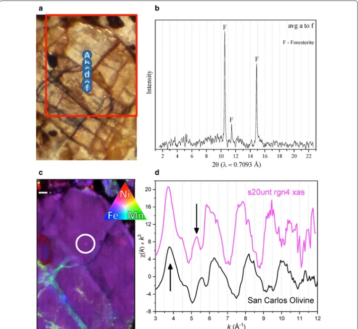
Figure 1 highlights the complementary use of µ-XRD and µ-XAS to identify solid phase minerals which contain
Ni. A high-resolution photograph (Fig. 1a) shows a min-eral in the petrographic thin section of sample “s20unt” region 4 upon which µ-XRF, µ-XRD, and µ-XAS were carried out. The red box on the photograph indicates the approximate boundaries of the µ-XRF map. Spots A through F indicate the locations where µ-XRD pat-terns were obtained. The µ-XRD patpat-terns were averaged together to improve the signal-to-noise ratio (Fig. 1b). The tricolored µ-XRF map is shown in Fig. 1c with Ni in
red, Fe in blue, and Mn in green. The µ-EXAFS spectrum was collected at the location of the smaller white circle and is shown along with a bulk-EXAFS spectrum of San Carlos Olivine for comparison in Fig. 1d. Ni K-edge bulk-EXAFS data of San Carlos Olivine [64] were digitized [65] and rebinned at 0.05 Å−1 in k-space.
Figure 1 serves as an example of Ni distributed in a constant and homogeneous manner throughout the solid phase of a large mineral particle (purple color in the tricolor map), which is hundreds of micrometers in the x, y directions (the scale bar is 30 μm). This mineral is off-white in color with several veins perpendicular to each other (see photograph). The veins accumulate Mn in some areas. Only three diffraction peaks were produced from the averaged μ-XRD spectra of this mineral, even though this is an average of six diffraction spectra “A–F”. The lack of multiple diffraction peaks commonly occurs in μ-XRD data (see Additional file 1: Text S2.2 for further discussion). The lack of peaks is because the sample and beam are stationary, so the X-ray beam does not reflect of all the mineral lattices. For this particular spot, both μ-XRD and μ-XAS data were collected. The diffraction peaks correspond to forsterite, which is a nesosilicate mineral in the olivine group. This was the only identifi-cation of forsterite in this work; however, forsterite was identified in the bulk and silt fractions of the “s20unt” soil [15].
Nesosilicate minerals are different from phyllosilicate minerals and inosilicate minerals because the silica tetra-hedra are held together only by electrostatic forces, thus they weather readily in soils [66, 67]. Inosilicate (or chain
silicate) minerals have chains of silica tetrahedra that share two corner oxygen atoms. An increasing number of chains give greater resistance to weathering. The phyl-losilicate minerals contain layers of silica tetrahedra with three oxygen atoms sharing between two tetrahedra. This provides even further resistance to weathering [66]. For-sterite is a Mg-rich mineral common to ultramafic rocks. It associates with enstatite, magnetite, antigorite, and chromite [68]. Thus, its occurrence here is understand-able, and Ni substitution into the olivine/forsterite struc-ture is common.
The physical location of the μ-EXAFS spectrum “s20unt rgn4 xas” is indicated by the small white inner circle on μ-XRF the map. Both the μ-EXAFS and μ-XANES (Fig. 2a, b) spectra from this spot display features unique to forsterite. In the μ-EXAFS spectrum, there is a steep (elongated) first peak with a maximum at ca 3.7 Å−1
(Fig. 1d, see arrow). The elongated peak is unique to for-sterite and not seen in the other samples (Fig. 2). The elongated peak at ca 3.7 Å−1 is similar to other work
which studied Ni distribution San Carlos Olivine [64]. Another peak of interest in the sample is at ca 5.3 Å−1
(ca 5.5 Å−1 in the San Carlos Olivine spectrum) and
is indicated with another arrow. There is a distinct upward peak at this energy. The similarity of the struc-tural features (such as peaks and shoulders) between the μ-EXAFS from this study and the bulk-EXAFS of San Carlos Olivine provides evidence of Ni incorpora-tion into this olivine-group mineral. The phase of the major oscillations in the San Carlos Olivine spectrum is slightly longer than those seen in the μ-EXAFS data.
The elongated peaks at ca 3.7 Å−1 line up well between
the two spectra, but the next peak at arrow ca 5.3 Å−1 is
slightly shifted to ca 5.5 Å−1 in the San Carlos Olivine.
The slight contraction of the major oscillations in the μ-EXAFS spectrum versus the San Carlos Olivine spec-trum is perhaps due to differences in the ratios of trace metals (Fe, Mn, and Ni, versus Mg) incorporated into the two different samples. The spectroscopic and diffraction data in Fig. 1 corroborate each other to show homogene-ous incorporation of Ni into forsterite. The major distin-guishing oscillations in μ-EXAFS spectrum at ca 3.7 and ca 5.3 Å−1 also match up well with those the of another
forsterite mineral standard [27].
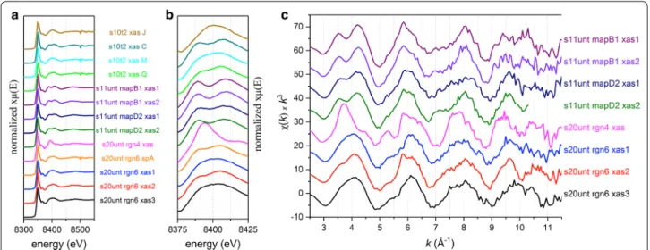
The major distinguishing oscillations of each µ-XAS spectra from all samples can be compared in Fig. 2, including both µ-XANES and µ-EXAFS spectra. In total, there are 13 µ-XANES spectra (Figs. 2a, b) and 8 µ-EXAFS spectra (Fig. 2c). The close up of the XANES region (Fig. 2b) illustrates differences in the split shoul-der at 8400 eV. This split is also part of the EXAFS region, and this energy (8400 eV) translates to 3.7 Å−1 in the
EXAFS region. At this wavenumber, a large indentation is present in the first oscillation of the spectra. Forsterite contains the elongated peak not seen in the samples. This elongated peak is at a similar location to the first peak of the split shoulder feature in other samples.
Lighter elements, such as Al atoms, allow for the appearance of the split in the first EXAFS oscillation [47], similarly to the effect of Mg atoms common in ultramafic serpentine minerals. The split can be readily seen for transition metals bound in the octahedral layer of clays and in Al-modified phyllosilicates [29, 48, 49]. Ultramafic parent materials are high in Mg; thus Mg would likely be the dominant light-weight cation in the octahedral layer. Mg concentrations for soils “s10t2”, “s11unt”, and “s20unt” were 15,700, 23,600, and 13,900 mg kg−1, respectively
(Additional file 1: Table S1). Thus, a split shoulder at this particular energy indicates Ni incorporation into the octahedral sheet of a layered silicate mineral, such as a phyllosilicate including clinochlore or lizardite [15]. In EXAFS spectra of “Ni-rich” and “Ni-poor” serpentine minerals [27], the former lack an indentation in the first oscillation, and the latter display an indentation similar to the serpentine mineral standards used in this study.
Figures 1 and 2 illustrate the manner in which data in Additional file 1 were analyzed and facilitate simul-taneous comparison of µ-XAS data from all samples, respectively. The results of each sample (including
µ-XRF µ-XRD µ-XAS) are given in Additional file 1:
Figures S1 through S24 along with detailed accompany-ing text. Figures in Additional file 1 have been summa-rized in Tables 1, 2, and 3, and summary discussions and
conclusions are in “Summary of μ-XRD”, “Summary of
μ-XRF”, and “Summary of μ-XAS”. Table 1 is a summary of all the minerals identified by µ-XRD in each sample and spectrum. Table 2 is a summary of Ni and elemen-tal distributions in µ-XRF maps. Table 3 is a summary of all the µ-XAS data collected, including both µ-XANES and µ-EXAFS. Results from LCF of both µ-XANES and µ-EXAFS spectra are given in Table 3, while the spec-tral fits themselves are given in their corresponding fig-ures in Additional file 1. In total, five spots possess both microfocused spectroscopic (µ-XAS) and diffraction data (µ-XRD).
Summary of µ‑XRD
Data in Table 1 summarize the results from each diffrac-togram. Because Ni is naturally occurring in serpentine soils and lateritic profiles, it is not deposited from aero-sols emitted by smelters or other anthropogenic sources. Thus, in addition to being sorbed to clay mineral sur-faces, Ni is commonly incorporated into the crystal lat-tices of silt and sand-sized particles of the parent and secondary minerals [1, 15]. The µ-XRD data indicate that Ni was often located in the octahedral layer of serpentine minerals (for example, lizardite) and other minerals such as chlorite, which is another layered phyllosilicate min-eral with octahedral structure similar to lizardite. Micro-focused-XRD spots close in physical proximity but with elemental heterogeneity were commonly seen to produce similar µ-XRD patterns (Additional file 1: Figures S10– S12a, b). Enstatite, chlorite, pargasite, antigorite, lizar-dite, and phlogopite integrated various amounts of Ni and Fe over the micrometer scale (Additional file 1: Fig-ures S11––S15, S16b–S18, and S23b). Enstatite is a chain inosilicate mineral also found in the bulk-XRD patterns of “s11unt” [15]. It is a ferromagnesian pyroxene mineral common to mafic rocks [1, 68]. Chlorite minerals, such as clinochlore and chamosite, were important Ni spe-cies in multiple samples. Over a 500 µm µ-XRD transect, chamosite and phlogopite illustrated large difference in elemental composition; Ni content increased six to seven times within the same transect (Additional file 1: Figure S10). Lizardite was identified multiple times as in impor-tant host for Ni. This is reasonable because Ni can sub-stitute for Mg2+ in olivine, pyroxenes, and serpentine minerals [1]. Chlorite and enstatite also incorporated varying amounts of Ni and Fe in their structures, often within the same mineral (Table 1).
Table 1 A summary of all minerals identified by µ-XRD in each sample and spectrum
Figure #
Mineral →
Spot Label ↓ Goeth
ite
He
ma
tite
Ma
gne
tite
Ma
ghe
mi
te
An
tigor
ite
Liz
ar
di
te
Clin
oc
hl
or
e
Chlor
ite
Cha
mo
si
te
En
st
at
ite
Phl
ogopi
te
Pa
rgasi
te
Fors
teri
te
Epid
ot
e
Geik
ie
lite
Grossular Chrom
ite/
Zin
coch
ro
mi
te
Qu
ar
tz
no
peak
s
Elements at Spot
Figure S4b s10t2 region 1 map A x Ni,Fe
Figure S4b s10t2 region 1 map B x Ni,Mn
Figure S5 s10t2 region 4 map A x Fe, Ni(low)
Figure S6b s10t2 region 5 mini map J avg 11 to 15 x x x Ni,Fe Figure S7 s10t2 clay particles map avg 1,2,3 x x x clay fraction
Figure S8b s10t2 silt particles map 1 x Ni
" " 3 x Ni
" " 6 x Ni
" " 7 x x Ni
" " 8 x x Fe
" " 9 x x Fe
" " 11 x x Cr,Fe,Zn,As
" " 13 x Ni,Fe
" " 14 x Mn
Figure S9b s10t2 medium sand map 1 x x x Ni,Fe
" " 2 x Ni
" " 3 x Ni
" " 8 x Ni
" " 9 x Ni
" " 5 x x x Ni,Fe
" " 6 x x Ni
" " 7 x Ni,Mn
" " 10 x Ni,Mn
" " 11 x Cr,Zn
" " 12 x Cr,Zn
" " 13 x x x Fe,Ni(low)
" " 16 x x Fe
Figure S10 s11unt map A1 avg 77 to 82 x x x Fe
" " avg 02 to 08 x x x Fe
" " avg 75 to 81 x x x Ni,Fe
" " avg 51 to 61 x x x Ni,Fe
Figure S11 s11unt map A2 avg 39 & 40 x x Fe
" " avg 51 to 53 x x Ni,Fe
" " avg 64 & 65 x x Ni,Fe
Figure S12b s11unt map B1 2840 x x Fe
" " 10421 x x Ni
" " 10432 x x Ni(low),Fe
Figure S13 s11unt map B2 avg 61 to 69 x Fe
" " avg 75 & 76 x x Ni,Fe
" " y05 x x Ni,Fe
Figure S14 s11unt map C 426 x x Ni,Fe,Zn
" " avg 14 to 20 x Ni,Fe,Zn(low)
" " 3165 x Ca
" " 396 x Ca
" " 390 x x Ni,Fe,Mn
Figure S15 s11unt map D1 avg 67 to 73 x x Fe
" " avg 355 to 515 x x Ni,Fe
Figure S16b s11unt map D2 445 x Fe
" " 436 x Ni,Mn,Fe(low)
" " 409 x Ni,Mn
Figure S17 s11unt map E 4090 x x Ni,Fe
" " avg 59 to 65 x Ni
" " avg 47 to 50 x x Fe
" " avg 83 to 89 x Cr,Zn
Figure S18 s11unt map F 95 x x Ni,Fe
" " avg 13 & 15 x x Ni,Fe
" " avg 01 to 05 x x Ni,Fe
" " avg 95 to 96 x x Ni,Fe
" " y9606 x Fe,Mn
" " y9615 x Ni,Fe
Figure S19b s11unt silt particles map 1 x x Ni
" " 2 x Ni
" " 4 x x Ni
" " 5 x Ni,Mn
" " 7 x Ni,Mn
" " 8 x x Ni,Fe(low)
" " 10 x x Ni,Fe(low)
" " 17 x Ti
" " 18 x Ca
" " 21 x x Fe
Figure S19c s11unt silt particles high-res 1 x x Ni,Mn
" " 2 x x Ni,Mn
" " 4 x Ni,Mn
" " 5 x x x Fe
" " 7 x x Ni,Fe,Mn
" " 8 x Cr
Figure S20 s20unt region 1 map XRD1 transect x Fe(low)
Figure S21 s20unt region 3 map avg a to d x Ni,Mn
" " avg w1 & w2 x none
Figure S22 s20unt region 4 map avg a to f x Fe,Ni
Figure S23b s20unt region 6 spot A map avg 53,55,57 x x Ni # of occurrences 9 10 7 4 6 20 12 18 7 7 8 1 1 2 1 1 5 10 5
chamosite, which is rich in Fe2+. It can occur in serpen-tinite and ultramafic rocks and associates with olivine [68]. Chlorite integrated both Fe and Mn simultaneously
(Additional file 1: Figure S18) into its structure. Lizard-ite also simultaneously hosted Ni and Mn in its octahe-dral layer. Though, at discrete Ni/Mn hotspots, it was
Table 2 Summary of Ni and elemental distributions in each map
Several of the maps are smaller, higher resolution maps and thus not included in the last row tallies
Notes on elemental
distribution → sample↓ ANi B C D E F G H
diffuse with Fe
Ni diffuse with Mn
Ni hotspot with Fe
Ni hotspot with Mn
Ni
unassociated hotspots
Fe
unassociated hotspots
Mn
unassociated hotspots
Other unassociated hotspots
Figure S4a—s10t2 region 1 map x x x x x Cr
Figure S4b—s10t2 region 1 map x x x
Figure S5—s10t2 region 4 map x x x x Cr/Zn
Figure S6a—s10t2 region 5 map x x x x x x Cr
Figure S6b—s10t2 region 5 mini
map J x x Cr, Ti
Figure S6c—s10t2 region 5 mini map
M&C x x x x x Cr/Zn, Ti
Figure S6d—s10t2 region 5 mini
map Q x x x Cr/Zn, Ti
Figure S7—s10t2 clay particles map x x
Figure S8a—s10t2 silt particles map – – – – – – – –
Figure S8b—s10t2 silt particles map x x x x x Cr
Figure S9a—s10t2 medium sand
map – – – – – – – –
Figure S9b—s10t2 medium sand
map x x x x Cr/Zn
Figure S10—s11unt map A1 x x Ti
Figure S11—s11unt map A2 x x x x Cr/Zn, Ti
Figure S12a—s11unt map B1 x x x x
Figure S12b—s11unt map B1 – – – – – – – –
Figure S13—s11unt map B2 x x x Cr, Ti
Figure S14—s11unt map C x x x x Ti, Ca
Figure S15—s11unt map D1 x x x Zn
Figure S16a—s11unt map D2 x x x x x x
Figure S16b—s11unt map D2 – – – – – – – –
Figure S17—s11unt map E x x x x Cr/Zn, Ti
Figure S18—s11unt map F x x x Cr, Ti, Ca
Figure S19a—s11unt silt map – – – – – – – –
Figure S19b—s11unt silt map x x x x x
Figure S19c—s11unt silt high‐res x x Cr/Zn, Ti, Ca
Figure S20—s20unt region 1 map x x x x
Figure S21—s20unt region 3 map x x x x x x Cr/Zn/Fe
Figure S22—s20unt region 4 map x x x x x x Cr/Zn
Figure S23a—s20unt region 6 map x x x x x x x Cr/Zn, Ti
Figure S23b—s20unt region 6 spot
A map – – – – – – – –
Figure S23c—s20unt region 6 spot
B map – – – – – – – –
# of occurrences 19 7 14 17 12 21 12
Table 3 Summar y the L CF r esults fr om µ -EX AFS and µ -X ANES sp ec tr a Figur e Sample
Spot label on figur
e μ‑ XANES μ‑ EX AFS μ‑ XRD Split pr esen t Elemen ts a t spot (via µ ‑XRF map ) LCF r esults (standar ds in Table S2) R‑ fac tor fr om L CF F‑ test v alue for n + 1 standar ds Delta E0 (eV ) Figur e S6b s10t2 r eg
ion 5 mini
map J xas J x x no N i, F e 74% ir on o xide (N i-hematit e) 25% ir on o xide (N i-f er ri pH7) 0.0004 5.4% N/A Figur e S6c s10t2 r eg
ion 5 mini
map M&C xas M x no N i, M n 75% la yer ed ser
-pentine mineral (Ni–Al LDH) 27% manganese oxide (N
iT
C bir
n)
0.0003
N/A
0.421 (0.013) 0.429 (0.034)
Figur
e S6c
s10t2 r
eg
ion 5 mini
map M&C xas C x ye s N i, F e (lo w) 83% la yer ed ser
-pentine mineral (Ni-ser
p 5811) 17% ir on o xide (N i-fer rih ydr ite) 0.006 N/A N/A Figur e S6d s10t2 r eg
ion 5 mini
map Q xas Q x ye s N i, M n, F e 50% La yer ed ser
-pentine mineral (Ni-ser
p 5811) 49% ir on o xide (N i-hematit e) 0.0005 N/A
0.468 (0.024) 0.435 (0.055)
Figur
e S12a
s11unt map B1
xas1 x x x ye s N i, F e (lo w), M n (lo w) 39% la yer ed ser
-pentine mineral (Ni-g
ibbsit e) 72% la yer ed ser
-pentine mineral (Ni-ser
p 5811) 0.084 80% N/A Figur e S12a
s11unt map B1
xas2 x x ye s N i, F e, M n (lo w) 37% la yer ed ser
-pentine mineral (Ni-g
ibbsit e) 74% la yer ed ser
-pentine mineral (Ni-ser
p 5811) 0.107 64% N/A Figur e S16a
s11unt map D2
xas1 x x x ye s N i, M n 79% la yer ed ser
-pentine mineral (Ni-g
ibbsit
e)
10% manganese oxide (N
i-RS bir n) 0.044 28% N/A Figur e S16a
s11unt map D2
xas2 x x ye s Ni 70% la yer ed ser
-pentine mineral (Ni-g
ibbsit e) 30% la yer ed ser
-pentine mineral (Ni-ser
p 5811)
0.061
41%
Samples with µ
-X
ANES and µ
-EX
AFS da
ta ar
e iden
tified along with those samples wher
e c omplemen tar y µ -XRD spec tr a w er e obtained . T he pr esenc
e of a split shoulder a
t 8400 eV and 3.7 Å
−
1 for µ
-X
ANES and µ
-EX AFS da ta, r espec tiv ely
, is also indica
ted along with the elemen
ts pr esen t a t tha t loca tion ac cor
ding the µ
-XRF maps . Er ror v alues f or E0 ar e adjac en
t in par
en
theses (see A
dditional file 1 : T ex t S2.4.) Table 3 (c on tinued) Figur e Sample
Spot label on figur
e μ‑ XANES μ‑ EX AFS μ‑ XRD Split pr esen t Elemen ts a t spot (via µ ‑XRF map ) LCF r esults (standar ds in Table S2) R‑ fac tor fr om L CF F‑ test v alue for n + 1 standar ds Delta E0 (eV ) Figur e S22 s20unt r eg ion 4 map rg n4 xas x x x no Fe , N i See F ig . 1 N/A N/A N/A Figur e S23b s20unt r eg ion 6
mini map A
spA x x ye s Ni 67% la yer ed ser
-pentine mineral (Ni–Al LDH)
33% la
yer
ed ser
-pentine mineral (Ni-ser
p 5811)
0.0006
≪
1%
0.400 (0.078) 0.400 (0.033)
Figur
e S23c
s20unt r
eg
ion 6
mini map B
xas1 x x no N i, F e 46% la yer ed ser
-pentine mineral (Ni-g
ibbsit e) 55% ir on o xide (N i-hem pH7) 0.068 9% N/A Figur e S23c s20unt r eg ion 6
mini map B
xas2 x x ye s N i, F e (lo w) 42% la yer ed ser
-pentine mineral (Ni-silicat
e)
75% la
yer
ed ser
-pentine mineral (Ni-ser
p 5811) 0.062 10% N/A Figur e S23c s20unt r eg ion 6
mini map B
xas3 x x no N i, F e lo w), M n
73% manganese oxide (N
i-RS bir n) 34% la yer ed ser
-pentine mineral (Ni-ser
p 96)
0.037
8%
common that no diffraction peaks could be observed (Additional file 1: Figures S4b and S9b). Some improve-ment in diffraction patterns can be obtained by “rocking” the sample several microns under the X-ray beam in the x, y direction while collecting data. In lizardite, Ni was also independent of other trace metals (Additional file 1: Figures S16a, b, S19b). These findings agree with lit-erature where serpentine minerals contained a relatively consistent amount of Ni. For example, in an Albanian ultramafic toposequence serpentine minerals contained about 0.3% Ni while Ni content in smectites ranged up to 4.9% [69]. The serpentine soils of this toposequence developed on serpentinized harzburgite, and harzburgite is also a common type of peridotite parent material in the serpentine soils of the Klamath Mountains [13].
Ni was associated with Fe in a variety of morphological fashions, ranging from agglomerated minerals, where a combination of hematite, clinochlore, and goethite were present (Additional file 1: Figure S6b), to larger discrete particles where Ni was in forsterite, goethite, and hema-tite. Goethite and hematite are common secondary Fe oxides that form during weathering processes of serpen-tine soils [1]. Other µ-XRD results also indicated Ni accu-mulation in goethite (Additional file 1: Figure S8b). Lower amounts of Ni were in hematite than in goethite on the µ-XRF maps. Goethite was identified in the silt particle size fraction (25–45 µm) together with lizardite and anti-gorite in the same diffractograms (Additional file 1: Fig-ure S19b), illustrating that on the tens of micrometers scale these minerals can be closely associated and both host Ni and Fe.
Thus mixtures of Fe oxides and serpentine minerals were detected by µ-XRD; another example is in Addi-tional file 1: Figure S9b, “spot 1” and “spot 5”. This close physical association of minerals indicates that perhaps during lizardite weathering, as Fe2+ leaches out it can oxidize and precipitate to form goethite. Ni accumulation in iron oxides has been found in other ultramafic profiles, for example, a lateritic regolith [27]. Ni in primary silicate minerals, such as olivine in the bedrock, was incorpo-rated into the structures of secondary phyllosilicate min-erals and iron oxides, such as serpentine and goethite, respectively. This occurred in the lower portion of the regolith (saprolite). In the upper portion of the regolith profile (the lateritic portion) Ni was principally located into the goethite structure. Manganese oxides also hosted a significant portion of Ni in the transition laterite zone [27].
It was uncommon for Ni and Zn to associate, but evi-dence is given for the inclusion of Zn into the layered structures of clinochlore and antigorite (Additional file 1: Figures S14); although, trace metal substitution (such as Ni, Fe, or Mn) into the antigorite structure was not
always observed, such as in Additional file 1: Figure S21 where antigorite likely rich in only Mg was identified. Cr hotspots could often be identified as chromite mineral via µ-XRD (for example, Additional file 1: Figure S9b). The presence of Ti and Ca rich minerals were also identi-fied by µ-XRD (Additional file 1: Figure S19b), illustrating the versatility of the µ-XRD technique.
Summary of µ‑XRF
The maps cover a combined 25 different regions in the samples. Several of the maps are smaller, higher reso-lution maps and thus not included in the summary tal-lies at the bottom of Table 2. In Table 2, Ni distribution was separated into five different trends which commonly occurred in the samples. In column A, “Ni diffuse with Fe” indicates Ni distribution at low but homogeneous levels over broad areas of a map. This distribution can be in Fe oxide clays or in larger mineral surfaces such as lizardite, antigorite, clinochlore, or forsterite. In column B, “Ni diffuse with Mn” indicates areas where Ni and Mn associate in amorphous regions, not bound by the edges of mineral surfaces seen in the accompanying photo-graphs. In column C, “Ni in hotspots with Fe” indicates small, discrete areas where Ni and Fe associate. In col-umn D, “Ni in hotspots with Mn” indicates areas where Ni and Mn associate in discrete regions typically bound by the edges of mineral surfaces. In column E, “Ni unas-sociated hotspots” indicates areas where Ni is not associ-ated with other elements in the µ-XRF maps. Generally these regions are discrete, well bounded, and not amor-phous. In the remaining columns (F, G, and H), other ele-ments and elemental associations are indicated.
The tallies at the bottom of Table 2 indicate the per-cent of occurrences for a particular distribution trend. In 76% of the maps, Ni was associated with Fe in a diffuse manner, either with Fe oxides or in the lattice structure of larger minerals such as lizardite, antigorite, clino-chlore, or forsterite. In only 28% of the observations, Ni was associated with Mn in a diffuse manner. Thus, in the µ-XRF maps, Ni was more often associated in a diffuse fashion with Fe than with Mn. This is likely due to the high content of iron and iron oxides in these soils; each soil contained goethite and/or hematite in its bulk-XRD pattern [15]. Additionally, the amount of Fe in each soil is much higher than Mn; Fe concentrations are about one order of magnitude or more than Ni for all three soils, and Ni concentrations were sometimes twice as high as Mn (Additional file 1: Table S1).
red goethite particles identified by µ-XRD (Additional file 1: Figure S4a). Mn hotspots were often correlated with Ni, and often Mn was densely associated with Ni in the µ-XRF maps in both diffuse and discrete areas (Addi-tional file 1: Figure S6d). Interestingly though, each time Ni and Mn associated densely in discrete black minerals, no or few diffraction peaks were produced (Additional file 1: Figures S4b “spot B”, Additional file 1: Figures S9b “spot 7 and 10”, and Additional file 1: Figures S21 “avg a–d”). Mn was seen to accumulate not only in veins of larger minerals (Figs. 1 and Additional file 1: Figure S22) but also discretely inside the bulk of minerals and within agglomerated Fe oxides. However, it is not necessary that Ni associate with any trace metals; 48% of the mapped regions contained unassociated Ni hotspots. The abun-dance of Fe in these samples, in terms of Fe oxide clays and minerals such as goethite and magnetite, yielded a high occurrence of unassociated Fe hotspots (84%). Lastly, 48% of the regions contained unassociated Mn hotspots. Thus in different locations, Ni, Fe, and Mn were associated together and also distributed independently of each other; their trends were categorized into eight groups (A–H) in Table 2.
Ni generally did not associate with Cr, Zn, Ca, or K. Though, Zn correlated with several Cr hotspots. Ni and Cr essentially never correlated with each other in the µ-XRF maps. The exception to Ni and Cr correlation was in the clay fraction of “s10t2” (Additional file 1: Figure S7) where no resolution of discrete particles was possi-ble from the µ-XRF maps. The clay size fraction contains particles (≤ 2 µm) that are smaller than the X-ray beam (2 µm at SSRL). Information on elemental distributions cannot be gleaned when particle sizes are smaller than the beam, which can also be caused by grinding samples in a mortar/pestle. Thus for samples used in this study it is not recommended to grind samples because this can homogenize the sample and prevent correlations of dif-ferent elements. A useful aspect of µ-XRF mapping is that elements in the maps can be used to eliminate mineral hosts with similar matching diffraction peaks but which are not compatible given the fluorescing elements. Addi-tionally, the µ-XRF maps can be used to limit the num-ber of standards used in LCF. For example, if a µ-XRD or µ-EXAFS spectrum was obtained from a spot high in Ni and Mn fluorescence but very low in Fe, all the Fe oxide mineral standards (goethite, ferrihydrite, magnetite, et cetera) could be excluded from matching peaks or LCF routine, respectively.
Summary of µ‑XAS
Table 3 is a summary of the µ-XAS data and LCF results. Ni speciation was dominated by serpentine mineral standards, such as lizardite, and Ni bound (either via
surface adsorption or precipitation/incorporation into mineral structure) with iron oxides, such as goethite, hematite, and ferrihydrite. In seven of the eight spectra that displayed a split shoulder feature at 8400 eV, there is a decrease the counts per second (CPS) of Fe or Mn or low overall CPS of Fe, Mn, or Ni. When other trace met-als such as Fe and Mn are low and Ni is the predominant fluorescing metal in the µ-XRF maps, the split shoulder generally occurs. Spectral features in the µ-XANES and µ-EXAFS data, such as the split at 8400 eV and 3.7 Å−1,
respectively, indicate that Ni is located in the octahe-dral layers of phyllosilicate minerals such as lizardite or a chlorite-group mineral; this is confirmed by µ-XRD in Additional file 1: Figures S12 spot “B1xas1”, Additional file 1: Figures S16 spot “D2xas1”, and Additional file 1: Figures S23b “spA”.
The presence of the split can be used to identify this specific type of local atomic environment. Ni is octahe-drally coordinated with oxygen in a sheet and has lighter elements such as Mg as the dominant second nearest neighbors (for example, Ni–O–Mg). Mg dominates as the light element in lizardite [Mg3Si2O5(OH)4]. This split
shoulder is clearly visible in lizardite mineral standards [15], and it is common for trace metals in phyllosilicates [70–74]. The split shoulder can often occur where trace metals such as Ni or Zn are present in phyllosilicates [15, 29]. See references [47–49] for more discussion on the formation of this split shoulder feature.
For example in Additional file 1: Figure S6c at spot “M”, because Mn (Z = 25) is heavier than Mg (Z = 12) no split-ting would occur if Ni were present in chlorite. Ni could be associated with a layered Mn oxide, such as birnessite, or a layered phyllosilicate mineral such as chlorite, which can be heavily substituted with Mn in the octahedral layer. The LCF results agree with this hypothesis because the manganese oxide standards were consistently ranked as important components in the best fits for this spot. The final fit however included NiAl-LDH (75%) and Ni sorbed to triclinic birnessite (NiTC Birn 27%). This result does not mean that NiAl-LDH is the actual species in the sample; rather, the NiAl-LDH standard is being used as an analogue for another Ni-rich layered mineral where Ni is in the octahedral sheet, such as lizardite or a chlorite-group mineral. The NiAl-LDH standard is representative of Ni in the 2 + oxidation state, octahedrally coordinated by ~ 6 oxygen atoms, and located in the octahedral sheet of a layered mineral, which are three characteristics that make it a good analogue for Ni substituted into a serpen-tine mineral. Thus at spot “M”, Ni is likely associated with a Mn-rich serpentine mineral. Another example where there is a decrease in the split shoulder is in Additional file 1: Figure S23b, where Ni is the only dominant fluo-rescing trace metal; the split is not as pronounced as in other spectra likely because of the relatively high Ni CPS which would be found in a Ni-rich phyllosilicate mineral.
By averaging the µ-XAS LCF results from both µ-EXAFS and µ-XANES, a comparison was made to
bulk-XAS LCF results previously published [15] for
these three soils. This comparison helps to determine if the microfocused data are representative of the bulk soil. Bulk-XAS LCF results showed higher Fe-oxide con-tents in “s10t2” than in other samples [15]. The averaged µ-XAS LCF data yielded a similar result; of the three soils, “s10t2” also has the highest percentage of Fe oxides; the “Iron Oxides” category composed 41% of all “s10t2” fits, while the “Layered Serpentine Minerals” category was 52%, and the “Manganese Oxides” category was 7%. Additional file 1: Text S2.3 discusses the categories for each standard. In the bulk-LCF XAS results for “s10t2”, Fe oxides were 42%, serpentine and ultramafic minerals were 23%, and Ni adsorbed to phyllosilicates composed 34% [15]. Ni adsorbed to phyllosilicates was not identi-fied by LCF of the µ-XAS data.
Differences in averaged µ-XAS LCF versus bulk-XAS LCF can be influenced by sampling bias. Inadvertently producing sampling bias in microfocused work can be caused by only obtaining data from “hotspots” of the ele-ment of interest. For this work, different morphological and elemental associations of Ni including diffuse and dense associations and various metal amounts (that is, CPS) were analyzed to decrease sampling bias and obtain
a more representative view of Ni speciation. These mor-phologies and elements are identified in Tables 1 and 2. Microfocused-XRF maps from petrographic thin sections helped to discern between Ni sorbed to clay minerals such as Fe oxides and larger mineral phases based on the morphology of the fluorescence pattern in relation to the high-resolution photographs.
For “s11unt”, averaging the µ-XAS LCF results deter-mined that “layered serpentine minerals” composed 100% of the fits while “Manganese Oxides” just 3%. The total value is over 100%, which is possible as explained in Additional file 1: Text S2.4. These averages for “s11unt” are similar to those for averaged bulk-XAS LCF, where serpentine minerals composed 83% to 96% of the bulk XAS spectra [15]. Thus for “s11unt”, there is good rep-resentation of the bulk soil and sample heterogeneity via the µ-XAS technique. Lastly, for “s20unt”, because of spectral similarities between Mn oxide standards and other standards, the bulk-XAS LCF value of the Mn oxide component was artificially increased [15], which made it quite different than the averaged µ-XAS LCF results of “s20unt”. For averaged µ-XAS LCF of “s20unt”, 74% of the fits could be attributed to “layered serpentine minerals”, 14% to “Iron Oxides”, and 18% to “Manganese Oxides”. Thus there was good representation of the bulk soil via the µ-XAS technique for two of the three soils.
In terms of combined LCF results from all three soils, averaged µ-XAS LCF values from all the fits indicated that standards in the “layered serpentine minerals” cat-egory consistently dominated, and on average they con-tributed to 76% of all LCF. Thus, for all locations analyzed by µ-XAS LCF, Ni speciation was dominated by layered phyllosilicate and serpentine minerals (76%), with smaller contributions on average from iron oxides (18%) and manganese oxides (9%).
Conclusion
On an 8 µm spatial scale, Ni and Mn were simultaneously present in lizardite and antigorite from µ-XRD patterns. Elemental fluorescence delineated and matched mineral morphology from high-resolution photographs. Elemen-tal distributions (for example, the fluorescence of Fe, Mn, and Ni) aligned between maps obtained from two dif-ferent beamlines (SSRL and NSLS). Data also indicate on the micrometer scale that serpentine minerals (for example, lizardite) can become embedded within larger iron oxide particles (for example, hematite). Additionally, diffraction peaks with goethite, magnetite, and lizardite were identified in the same µ-XRD spectrum, indicating that these minerals also can mix (associate) together on the micrometer scale.
particularly highlights how µ-XRD can be a key investiga-tive tool for identification of these minerals. The benefits of µ-XRD are that clear and discrete diffraction peaks can be matched with mineral phases in a prudent fashion and correlated to elements, such as Fe, Mn, Ni, Zn, and Cr in the µ-XRF maps. A more comprehensive and accu-rate dataset for Ni speciation was possible by combining µ-XRD with µ-XAS. The broader geochemistry commu-nities which focus on trace metal speciation in geologi-cal materials including soils and sediments using these microfocused techniques can find useful examples here of how to couple µ-XAS and µ-XRD together.
Previous work on these and other related serpentine soil samples focused on bulk physicochemical characteri-zation and bulk-EXAFS spectroscopy to characterize Ni in the whole soil and various particle size fractions [15]. The current work takes a different approach and had the objective to identify minerals which integrate Ni and Ni associations with other metals such as Fe, Mn, Zn, and Cr on the micrometer spatial scale. Of all the diffracto-grams analyzed for this work (over 500) and the result-ing µ-XRD spectra (88 total), a general summary can be made for Ni association with different mineral phases. Of the 88 µ-XRD spectra, 55 of those are from miner-als that contained Ni to some degree, either low or high CPS (Table 1). From those 55 spectra, 93 minerals were identified; often the same mineral was identified multiple times. For example, goethite was identified 9 times, and those 9 times it was present with Ni (Table 1). Taking the 93 minerals in which Ni was found and grouping those minerals into the categories used for LCF (Additional file 1: Text S2.3), we find good agreement between aver-aged µ-XAS data and µ-XRD data. For example, goethite, hematite, and magnetite are all iron oxides, and in total, iron oxides composed 17% of all minerals which hosted Ni as identified via µ-XRD. This is very similar to the 18% determined by the average of all µ-XAS LCF results “Summary of μ-XAS”. Similarly, the rest of the minerals (from antigorite to forsterite in Table 1) are all serpentine and ultramafic related minerals; those minerals grouped together accounted for 71% of all Ni-rich minerals identi-fied via µ-XRD. This value is very similar to the 76% of Ni associated with the “Layered Serpentine Minerals” cat-egory calculated by averaged µ-XAS LCF results.
These minerals, whether iron oxides or layered phyl-losilicates such as lizardite or chlorite-group minerals, affect Ni release into solution and Ni mobility in the environment. These results are useful to researchers in the Ni hyperaccumulation community, researchers studying ultramafic laterites and regoliths, serpentine parent materials and their geochemical weathering products, or trace metal release from serpentine soils.
These are all important current and future research areas; characterizing the naturally occurring minerals which host Ni is essential to understanding the rela-tionship between serpentine soils, metal hyperaccumu-lating plants, trace metal mobility, and environmental risk. Further research on these soils using selective dis-solution techniques and desorption kinetics studies while varying redox conditions would assist in linking Ni release and mobility to the dominant Ni species in the solid phase.
Additional files
Additional file 1: Text S1. Organization of this Additional file 1. Text S2. Materials and Methods. Text S2.1. µ-XAS and µ-XRF data collection. Text S2.2. µ-XRD data collection and processing. Text S2.3. Description of Standards. Text S2.4. PCA, TT, LCF, and F-Test. Figure S1. sample “s10t2” thin section photograph overview of maps. Figure S2. sample “s11unt” thin section photograph overview of maps. Figure S3. sample “s20unt” thin section photograph overview of maps. Figure S4a. s10t2 region 1 map. Figure S4b. s10t2 region 1 map (cont.) with μ-XRD. Figure S5. s10t2 region 4 map with μ-XRD. Figure S6a. s10t2 region 5 map with μ-XANES. Figure S6b. s10t2 region 5 mini map J with μ-XRD & μ-XANES. Figure S6c. s10t2 region 5 mini map M&C with μ-XANES. Figure S6d. s10t2 region 5 mini map Q with μ-XANES. Figure S7. s10t2 clay particles map with μ-XRD. Figure S8a. s10t2 silt particles map. Figure S8b. s10t2 silt particles map (cont.) with μ-XRD. Figure S9a. s10t2 medium sand particles map. Figure S9b. s10t2 medium sand particles map (cont.) with μ-XRD. Figure S10. s11unt map A1 with μ-XRD. Figure S11. s11unt map A2 with μ-XRD. Figure S12a. s11unt map B1 with μ-XANES and μ-EXAFS. Figure S12b. s11unt map B1 (cont.) with μ-XRD. Figure S13. s11unt map B2 with μ-XRD. Figure S14. s11unt map C with μ-XRD. Figure S15. s11unt map D1 with μ-XRD. Figure S16a. s11unt map D2 with μ-XANES and μ-EXAFS. Figure S16b. s11unt map D2 (cont.) with μ-XRD. Figure S17. s11unt map E with μ-XRD. Figure S18. s11unt map F with μ-XRD. Figure S19a. s11unt silt particles map. Figure S19b. s11unt silt particles map (cont.) with μ-XRD. Figure S19c. s11unt silt particles high-resolution map with μ-XRD. Figure S20. s20unt region 1 map with μ-XRD. Figure S21. s20unt region 3 map with μ-XRD. Figure S22. s20unt region 4 map with μ-XRD, μ-XANES, and μ-EXAFS. Figure S23a. s20unt region 6 map. Figure S23b. s20unt region 6 mini map A with μ-XRD and μ-XANES. Figure S23c. s20unt region 6 mini map B with μ-XANES and μ-EXAFS. Figure S24. EXAFS and XANES standards spectra, see references in Table S2. Table S1. Physico-chemical Characteristics of Soil Samples. Table S2. Standards used in LCF. Additional file 2. Clay centrifugation calculations.
Abbreviations
XRF: synchrotron based microfocused-X-ray fluorescence mapping; µ-XRD: synchrotron based microfocused-X-ray diffraction; µ-XAS: synchrotron based microfocused -X-ray absorption spectroscopy; µ-EXAFS: microfocused extended X-ray absorption fine structure spectroscopy; µ-XANES,: micro-focused X-ray absorption near edge structure spectroscopy; LCF: linear combination fitting; PCA: principal component analysis; TT: target transforma-tion; CPS: counts per second; CCD: charge-coupled device; SSRL: Stanford Synchrotron Radiation Lightsource; NSLS: National Synchrotron Light Source; USA: United States of America.
Authors’ contributions
Author details
1 Delaware Environmental Institute (DENIN), University of Delaware, Newark,
DE 19716, USA. 2 Department of Plant and Soil Sciences, University of
Dela-ware, Newark, DE 19716, USA. 3 Chaney Environmental, Beltsville, MD 20705,
USA.
Acknowledgements
We wish to thank J. Hendricks his support. We also thank the beamline scien-tists and user operation offices for the services they provide. Y. Arai is kindly thanked for provision of several reference XAS spectra.
Competing interests
The authors declare that they have no competing interests. Availability of data and materials
The datasets supporting the conclusions of this article are included within the article and its additional files. The soil samples used in this study can be made available upon request for the next 5 years. Further information can be accessed by contacting the corresponding author.
Ethics approval and consent to participate Not applicable.
Funding
This research was supported in part by the National Science Foundation Experimental Program to Stimulate Competitive Research grant number EPS-0814251, University of Delaware fellowships, and the Donald L. and Joy G. Sparks fellowship. Use of the NSLS was supported by the US Department of Energy under contract No. DE-AC02-98CH10886. Use of the Stanford Syn-chrotron Radiation Lightsource is supported by the U.S. Department of Energy under contract No. DE-AC02-76SF00515.
Publisher’s Note
Springer Nature remains neutral with regard to jurisdictional claims in pub-lished maps and institutional affiliations.
Received: 2 March 2018 Accepted: 10 July 2018
References
1. Alexander B, Coleman RG, Keeler-Wolfe T, Harrison SP (2007) Serpentine geoecology of Western North America: geology, soils, and vegetation. Oxford University Press, Oxford
2. Hseu ZY, Lai YJ (2017) Nickel accumulation in paddy rice on serpentine soils containing high geogenic nickel contents in Taiwan. Environ Geo-chem Health 39(6):1325–1334
3. Tashakor M, Hochwimmer B, Brearley FQ (2017) Geochemical assessment of metal transfer from rock and soil to water in serpentine areas of Sabah (Malaysia). Environ Earth Sci 76(7):281
4. Oze C, Bird DK, Fendorf S (2007) Genesis of hexavalent chromium from natural sources in soil and groundwater. Proc Natl Acad Sci USA 104(16):6544–6549
5. van der Ent A, Baker AJM, Reeves RD, Chaney RL, Anderson CWN, Meech JA et al (2015) Agromining: farming for metals in the future? Environ Sci Technol 49(8):4773–4780
6. USGS (2018) U.S. geological survey mineral commodity summaries 2018. USGS, Reston, VA, p 200
7. USGS (2012) U.S. geological survey mineral commodity summaries 2012. USGS, Reston, VA, p 198
8. Raous S, Echevarria G, Sterckeman T, Hanna K, Thomas F, Martins ES et al (2013) Potentially toxic metals in ultramafic mining materials: identifica-tion of the main bearing and reactive phases. Geoderma 192:111–119 9. Snoke AW, Quick JE, Bowman HR (1981) Bear Mountain igneous complex,
Klamath Mountains, California: an ultrabasic to silicic cale-alkaline suite. J Petrol 22(4):501–552
10. Bird JM, Weathers MS (1975) Josephinite: specimens from the earth’s core? Earth Planet Sci Lett 28(1):51–64
11. Alexander EB, Ellis CC, Burke R (2007) A chronosequence of soils and vegetation on serpentine terraces in the Klamath mountains, USA. Soil Sci 172(7):565–576
12. Burt R, Fillmore M, Wilson MA, Gross ER, Langridge RW, Lammers DA (2001) Soil properties of selected pedons on ultramafic rocks in Klamath Mountains, Oregon. Commun Soil Sci Plant Anal 32(13–14):2145–2175 13. Alexander EB (2004) Serpentine soil redness, differences among
perido-tite and serpentinite materials, Klamath mountains, California. Int Geol Rev 46(8):754–764
14. Oze C, Fendorf S, Bird DK, Coleman RG (2004) Chromium geochemistry in serpentinized ultramafic rocks and serpentine soils from the Franciscan Complex of California. Am J Sci 304(1):67–101
15. Siebecker MG, Chaney RL, Sparks DL (2017) Nickel speciation in several serpentine (ultramafic) topsoils via bulk synchrotron-based techniques. Geoderma 298:35–45
16. Rinklebe J, Antić-Mladenović S, Frohne T, Stärk H-J, Tomić Z, Ličina V (2016) Nickel in a serpentine-enriched Fluvisol: redox affected dynamics and binding forms. Geoderma 263:203–214
17. Kierczak J, Pędziwiatr A, Waroszewski J, Modelska M (2016) Mobility of Ni, Cr and Co in serpentine soils derived on various ultrabasic bedrocks under temperate climate. Geoderma 268:78–91
18. van der Ent A, Cardace D, Tibbett M, Echevarria G (2018) Ecological impli-cations of pedogenesis and geochemistry of ultramafic soils in Kinabalu Park (Malaysia). CATENA 160:154–169
19. Echevarria G, Massoura ST, Sterckeman T, Becquer T, Schwartz C, Morel JL (2006) Assessment and control of the bioavailability of nickel in soils. Environ Toxicol Chem 25(3):643–651
20. Massoura ST, Echevarria G, Becquer T, Ghanbaja J, Leclere-Cessac E, Morel JL (2006) Control of nickel availability by nickel bearing minerals in natu-ral and anthropogenic soils. Geoderma 136(1–2):28–37
21. Centofanti T, Siebecker MG, Chaney RL, Davis AP, Sparks DL (2012)
Hyper-accumulation of nickel by Alyssum corsicum is related to solubility of Ni
mineral species. Plant Soil 359(1–2):71–83
22. Rinklebe J, Shaheen SM (2017) Redox chemistry of nickel in soils and sediments: a review. Chemosphere 179:265–278
23. Tashakor M, Modabberi S, van der Ent A, Echevarria G (2018) Impacts of ultramafic outcrops in Peninsular Malaysia and Sabah on soil and water quality. Environ Monit Assess 190(6):333
24. Noel V, Morin G, Juillot F, Marchand C, Brest J, Bargar JR et al (2015) Ni cycling in mangrove sediments from New Caledonia. Geochim Cosmo-chim Acta 169:82–98
25. Noel V, Juillot F, Morin G, Marchand C, Ona-Nguema G, Viollier E et al (2017) Oxidation of Ni-rich mangrove sediments after isolation from the Sea (Dumbea Bay, New Caledonia): Fe and Ni behavior and environmen-tal implications. ACS Earth Space Chem 1(8):455–464
26. Dublet G, Juillot F, Brest J, Noel V, Fritsch E, Proux O et al (2017) Vertical changes of the Co and Mn speciation along a lateritic regolith developed on peridotites (New Caledonia). Geochim Cosmochim Acta 217:1–15 27. Dublet G, Juillot F, Morin G, Fritsch E, Fandeur D, Ona-Nguema G et al
(2012) Ni speciation in a New Caledonian lateritic regolith: a quantitative X-ray absorption spectroscopy investigation. Geochim Cosmochim Acta 95:119–133
28. Fan R, Gerson AR (2011) Nickel geochemistry of a Philippine laterite examined by bulk and microprobe synchrotron analyses. Geochim Cosmochim Acta 75(21):6400–6415
29. Manceau A, Marcus MA, Tamura N, Proux O, Geoffroy N, Lanson B (2004) Natural speciation of Zn at the micrometer scale in a clayey soil using X-ray fluorescence, absorption, and diffraction. Geochim Cosmochim Acta 68(11):2467–2483
30. Manceau A, Marcus MA, Tamura N (2002) Quantitative speciation of heavy metals in soils and sediments by synchrotron X-ray techniques. In: Fenter P, Sturchio NC (eds) Applications of synchrotron radiation in low-temperature geochemistry and environmental science, vol 49. Mineralogical Society of America, Washington, D.C., pp 341–428 31. Jackson ML (1985) Soil chemical analysis—advanced course, 2nd edn.
University of Wisconsin, Madison
32. Gee GW, Or D (2002) Particle-Size Analysis. In: Dane JH, Topp GC (eds) Methods of soil analysis part 4 physical methods. Soil Science Society of America Book Series, Madison
colloidal material in soil suspensions using sedimentation field-flow fractionation. Environ Sci Technol 39(6):1731–1735
34. Whittig LD, Allardice WR (1986) X-Ray diffraction techniques. In: Klute A (ed) Methods of soil analysis: part 1—physical and mineralogical meth-ods. SSSA book series. Soil Science Society of America, American Society of Agronomy, Madison, pp 331–362
35. Webb SM (2011) The MicroAnalysis Toolkit: X-ray fluorescence image processing software. In: McNulty I, Eyberger C, Lai B, editors. Proceedings of the 10th international conference on X-ray microscopy. AIP conference proceedings. 1365. Amer Inst Physics, Melville, pp 196–9
36. Webb SM (2005) SIXpack: a graphical user interface for XAS analysis using IFEFFIT. Phys Scr T115:1011–1014
37. Ravel B, Newville M (2005) ATHENA, ARTEMIS, HEPHAESTUS: data analysis for X-ray absorption spectroscopy using Ifeffit. J Synchrotron Radiat 12:537–541
38. Hammersley AP. FIT2D V9.129 reference manual V3.1. ESRF internal Report. 1998; ESRF98HA01T
39. Hammersley AP, Svensson SO, Hanfland M, Fitch AN, Hausermann D (1996) Two-dimensional detector software: from real detector to ideal-ised image or two-theta scan. High Pressure Res 14(4–6):235–248
40. Crystal-Impact (2012) Match! 1.x, Crystal Impact GbR, Bonn. http://www.
cryst alimp act.com/match /Defau lt.htm
41. Grazulis S, Daskevic A, Merkys A, Chateigner D, Lutterotti L, Quiros M et al (2012) Crystallography Open Database (COD): an open-access collection of crystal structures and platform for world-wide collaboration. Nucleic Acids Res 40(D1):D420–D427
42. Grazulis S, Chateigner D, Downs RT, Yokochi AFT, Quiros M, Lutterotti L et al (2009) Crystallography open database—an open-access collection of crystal structures. J Appl Crystallogr 42:726–729
43. Downs RT, Hall-Wallace M (2003) The American mineralogist crystal structure database. Am Miner 88(1):247–250
44. Omanovic D, Pižeta I (2016) High frequency data treatment and visualiza-tion with ECDSOFT and OnLineMonitor. In: Obrador B, Jones ID, Jennings E (eds) NETLAKE toolbox for the analysis of high-frequency data from lakes (Factsheet 5). Technical report. NETLAKE COST Action ES1201, pp 23–27
45. Omanovic D, Branica M (1998) Automation of voltammetric meas-urements by polarographic analyser PAR 384B. Croat Chem Acta 71(2):421–433
46. Yamaguchi NU, Scheinost AC, Sparks DL (2002) Influence of gibbsite surface area and citrate on Ni sorption mechanisms at pH 7.5. Clays Clay Miner 50(6):784–790
47. Siebecker MG, Li W, Sparks DL (2017) The important role of layered dou-ble hydroxides in soil chemical processes and remediation: what we have learned over the past 20 years Advances in Agronomy, vol 147. Academic Press, Cambridge
48. Nachtegaal M, Scheidegger AM, Dähn R, Chateigner D, Furrer G (2005) Immobilization of Ni by Al-modified montmorillonite: a novel uptake mechanism. Geochim Cosmochim Acta 69(17):4211–4225
49. Schlegel ML, Manceau A (2007) Zn incorporation in hydroxy-Al- and Keg-gin Al-13-intercalated montmorillonite: a powder and polarized EXAFS study. Environ Sci Technol 41(6):1942–1948
50. Arai Y (2008) Spectroscopic evidence for Ni(II) surface speciation at the iron oxyhydroxides—water interface. Environ Sci Technol 42(4):1151–1156
51. McNear DH, Chaney RL, Sparks DL (2007) The effects of soil type and chemical treatment on nickel speciation in refinery enriched soils: a multi-technique investigation. Geochim Cosmochim Acta 71(9):2190–2208
52. Peltier E, Allada R, Navrotsky A, Sparks DL (2006) Nickel solubility and pre-cipitation in soils: a thermodynamic study. Clays Clay Miner 54(2):153–164 53. Peltier E (2010) Lelie Dvd, Sparks DL. Formation and stability of Ni–Al
hydroxide phases in soils. Environ Sci Technol 44(1):302–308
54. Scheinost AC, Sparks DL (2000) Formation of layered single- and double-metal hydroxide precipitates at the mineral/water interface: a multiple-scattering XAFS analysis. J Colloid Interface Sci 223(2):167–178
55. Zhu MQ, Ginder-Vogel M, Sparks DL (2010) Ni(II) sorption on biogenic Mn-oxides with varying Mn octahedral layer structure. Environ Sci Tech-nol 44(12):4472–4478
56. Wasserman SR, Allen PG, Shuh DK, Bucher JJ, Edelstein NM (1999) EXAFS and principal component analysis: a new shell game. J Synchrotron Radiat 6:284–286
57. Malinowski ER (1978) Theory of error for target factor-analysis with applications to mass-spectrometry and nuclear magnetic-resonance spectrometry. Anal Chim Acta Comput Tech Optim 2(4):339–354 58. Malinowski ER (1977) Determination of number of factors and
experi-mental error in a data matrix. Anal Chem 49(4):612–617 59. Calvin S (2013) XAFS for everyone. CRC Press, New York
60. Kelly SD, Hesterberg D, Ravel B (2008) Analysis of soils and minerals using X-ray absorption spectroscopy. In: Ulery AL, Drees LR (eds) Methods of soil analysis part 5 mineralogical methods, vol 5. Soil Science Society of America, Madison
61. Hamilton WC (1965) Significance tests on the crystallographic R factor. Acta Crystallogr A 18(3):502–510
62. Downward L, Booth CH, Lukens WW, Bridges F. A variation of the F-test for determining statistical relevance of particular parameters in EXAFS fits. In: Hedman B, Painetta P, editors. X-ray absorption fine structure-XAFS13. Aip conference Proceedings. 8822007. pp 129–131
63. Soper D (2015) Regularized lower incomplete beta function calculator.
http://www.danie lsope r.com/statc alc3/calc.aspx?id=37http://www. danie lsope r.com/statc alc3/calc.aspx?id=37. Accessed 8 May 2015 64. Galoisy L, Calas G, Brown GE (1995) Intracrystalline distribution of Ni in
San-Carlos olivine—an EXAFS study. Am Miner 80(9–10):1089–1092
65. Huwaldt JA, Steinhorst S. Plot Digitizer. version 2.6.8 ed. http://plotd igiti
zer.sourc eforg e.net20 15. Accessed 27 Oct 2015
66. Schaetzl RJ, Anderson S (2005) Soils: genesis and geomorphology. Cam-bridge University Press, CamCam-bridge
67. Allen BL, Hajek BF (1989) Mineral occurrence in soil environments. In: Dixon JB, Weed SB (eds) Minerals in soil environments, 2nd edn. Soil Sci-ence Society of America, Madison, pp 331–378
68. Anthony JW, Bideaux RA, Bladh KW, Nichols MC. Handbook of
mineral-ogy: mineralogical society of America, Chantilly. 20151-1110, USA. http://
www.handb ookof miner alogy .org/. Accessed 19 Jan 2017 69. Bani A, Echevarria G, Montargès-Pelletier E, Gjoka F, Sulçe S, Morel JL
(2014) Pedogenesis and nickel biogeochemistry in a typical Albanian ultramafic toposequence. Environ Monit Assess 186(7):4431–4442 70. Manceau A, Llorca S, Calas G (1987) Crystal-chemistry of cobalt and nickel
in lithiophorite and asbolane from New-Caledonia. Geochim Cosmochim Acta 51(1):105–113
71. Manceau A, Schlegel ML, Musso M, Sole VA, Gauthier C, Petit PE et al (2000) Crystal chemistry of trace elements in natural and synthetic goe-thite. Geochim Cosmochim Acta 64(21):3643–3661
72. Roberts DR, Scheinost AC, Sparks DL (2002) Zinc speciation in a smelter-contaminated soil profile using bulk and microspectroscopic techniques. Environ Sci Technol 36(8):1742–1750
73. Roberts DR, Ford RG, Sparks DL (2003) Kinetics and mechanisms of Zn complexation on metal oxides using EXAFS spectroscopy. J Colloid Interface Sci 263(2):364–376
74. Scheinost AC, Kretzschmar R, Pfister S, Roberts DR (2002) Combining selective sequential extractions, X-ray absorption spectroscopy, and prin-cipal component analysis for quantitative zinc speciation in soil. Environ Sci Technol 36(23):5021–5028