An ice flow modeling perspective on bedrock adjustment patterns of the Greenland ice sheet

The Cryosphere, 6, 1263–1274, 2012 www.the-cryosphere.net/6/1263/2012/ doi:10.5194/tc-6-1263-2012

© Author(s) 2012. CC Attribution 3.0 License.

The Cryosphere

An ice flow modeling perspective on bedrock adjustment patterns of

the Greenland ice sheet

M. Olaizola1,*, R. S. W. van de Wal1, M. M. Helsen1, and B. de Boer1

1_{Institute for Marine and Atmospheric research Utrecht, Utrecht University, The Netherlands} *_{now at: Centre for Ice and Climate, Niels Bohr Institute, University of Copenhagen, Denmark} Correspondence to: M. Olaizola ([email protected])

Received: 8 November 2011 – Published in The Cryosphere Discuss.: 11 December 2011 Revised: 9 October 2012 – Accepted: 10 October 2012 – Published: 7 November 2012

Abstract.

Since the launch in 2002 of the Gravity Recovery and Climate Experiment (GRACE) satellites, several estimates of the mass balance of the Greenland ice sheet (GrIS) have been produced. To obtain ice mass changes, the GRACE data need to be corrected for the effect of deformation changes of the Earth’s crust. Recently, a new method has been proposed where ice mass changes and bedrock changes are simultane-ously solved. Results show bedrock subsidence over almost the entirety of Greenland in combination with ice mass loss which is only half of the currently standing estimates. This subsidence can be an elastic response, but it may however also be a delayed response to past changes. In this study we test whether these subsidence patterns are consistent with ice dynamical modeling results. We use a 3-D ice sheet–bedrock model with a surface mass balance forcing based on a mass balance gradient approach to study the pattern and magnitude of bedrock changes in Greenland. Different mass balance forcings are used. Simulations since the Last Glacial Max-imum yield a bedrock delay with respect to the mass balance forcing of nearly 3000 yr and an average uplift at present of 0.3 mm yr−1. The spatial pattern of bedrock changes shows a small central subsidence as well as more intense uplift in the south. These results are not compatible with the grav-ity based reconstructions showing a subsidence with a max-imum in central Greenland, thereby questioning whether the claim of halving of the ice mass change is justified.

1 Introduction

Since the Fourth Assessment Report by the International Panel on Climate Change, which included a mass balance (MB) estimate for the Greenland ice sheet (GrIS) of−50 to −100 Gt yr−1from 1993 to 2003 (Lemke et al., 2007), sev-eral studies have been published showing an increased loss in MB. Estimates mostly range between−160 to−300 Gt yr−1 over the period 2002 to 2010 (Velicogna and Wahr, 2006; Wouters et al., 2008; Rignot et al., 2008; Velicogna, 2009; Tedesco et al., 2011). These values are compatible with the study presented by van den Broeke et al. (2009), where mass balance estimates inferred from GRACE data are compared with the mass budget method showing good agreement be-tween the two methods.

Recently, a lower MB estimate (−81 to−127 Gt yr−1over the period 2002 to 2008) inferred from GRACE data has been reported by Wu et al. (2010) (referenced as W10 hereafter). The authors proposed a new method to simultaneously esti-mate the glaciological isostatic adjustment (GIA) trend and the present mass loss from GRACE, while in previous stud-ies the GIA trend is removed a priori (e.g. Velicogna and Wahr, 2006; Velicogna, 2009). Using this new method, W10 showed a pattern of strong ice thinning at the margin of the GrIS and slight central thickening, in agreement with previ-ous results (Thomas et al., 2006). The authors also retrieved a geoid subsidence almost over the entire island, most pro-nounced in the center and with a small area of uplift in the northwest. Averaged over Greenland, the geoid change is es-timated to be−0.56±0.17 mm yr−1. An average subsidence as suggested by W10 would intuitively be the result of an increase in ice loading, either in the past or in the present.

1264 M. Olaizola et al.: Bedrock adjustment patterns of the Greenland ice sheet

Observed ice loading changes have been used by Fleming et al. (2004) to show the strong spatial variability in geoid changes, which do not support a strong subsidence in the center. In addition, there is presently no indication of an in-creasing surface mass balance (SMB) (Ettema et al., 2009) that could explain bedrock subsidence in the central part of the ice sheet. Therefore, we tested if a SMB variability in the past could be responsible for the inferred subsidence and whether ice thinning and bedrock subsidence can ex-ist simultaneously for the present-day (PD) Greenland ice sheet. Furthermore we analyzed whether the sign, magnitude and pattern of a vertical bedrock movement, as the one re-ported by W10, can be simulated by realistic reconstructions of the ice-sheet evolution. This is done with a coupled ice sheet–bedrock model driven by variations in mass balance focussing on bedrock changes. Comparable ice model stud-ies were carried out by Huybrechts and Le Meur (1999) and Tarasov and Peltier (2002). This paper differs from previ-ous ice modeling experiments, as the work by Simpson et al. (2011) and the earlier mentioned papers, in the sense that it uses a different mass-balance forcing and it makes a spe-cific comparison with the bedrock-change patterns and re-constructions by W10. From a different perspective, ice load-ing histories have been reconstructed based on uplift data, e.g. Peltier (2004), but those are independent of climate and mass balance.

We start with a description of the three different compo-nents of the 3-D ice sheet–bedrock model: the ice dynam-ics, the surface mass balance and the solid earth (Sect. 2). In Sect. 3, we present the results of the different simula-tions where we studied the relation between changes in ice thickness and the bedrock response. In order to find out if bedrock subsidence in the central part of Greenland could be the result of a SMB increase during the Holocene, for example due to the Little Ice Age (LIA), a series of ex-periments were performed that mimic climate fluctuations in the past. The first experiment (Sect. 3.1) schematically mimics climate fluctuations during the Holocene following a 1K-amplitude sine function with a 1000 yr period, and de-scribes a quasi steady-state behavior. To incorporate the in-fluence of the last glacial era, we carried out a second experi-ment (Sect. 3.2) adding a linear increase in temperature from glacial conditions to PD. This experiment was performed for two different bedrock models, the Elastic Lithosphere Re-laxed Asthenosphere (ELRA) model, used as the standard model in the rest of the experiments, and the more complex Self Gravitational Viscoelastic (SGVE) model (Le Meur and Huybrechts, 1996), to validate the ELRA model and to study the possible influence of the model choice in the resulting bedrock pattern. Finally, we implemented a temperature forc-ing based on ice core records for a more realistic experiment (Sect. 3.3).

2 3-D ice-sheet model

We use the 3-D thermo-mechanical ice-sheet model AN-ICE (van de Wal, 1996, 1999; Helsen et al., 2012) based on the shallow ice approximation (Hutter, 1983; Huybrechts and de Wolde, 1999). It has three components: the interac-tion between ice surface and atmosphere (the SMB), the ice sheet and the solid earth. Interactions between ice surface and atmosphere are treated with the SMB gradient method (Helsen et al., 2012), that allows the use of SMB fields from climate models and accounts for the height–mass balance feedback. The SMB (1958–2007) from the regional climate model RACMO2/GR (Ettema et al., 2009) is used as the ref-erence SMB field, and perturbations are applied based on local changes in surface elevation (Hs) that result from the ice-sheet model. To enable an additional perturbation due to external temperature forcing, a variation in the annual sur-face temperature1T is divided byγ, the temperature lapse rate that results from a linear regression between elevation and temperature (γ= −7.3743 K km−1). In this way,1T is translated to a change in surface elevation (1H=1T /γ). Taking this into account, the SMB is calculated by

SMB=a+b(Hs+1T /γ ), (1)

whereaandbare local coefficients.

With the SMB gradient method, a spatially homogeneous climatic temperature perturbation is transferred into a region-ally variable SMB field. The response of the SMB to these perturbations in a specific grid point depends on the sign and magnitude of the SMB gradient (parametersbablandbaccin Helsen et al. (2012)). This response is quite straightforward in the ablation area where an increase in temperature leads to a SMB decrease. The magnitude of this response depends on the spatially variable parameterbabl. In the accumulation area, values of bacc can be either positive or negative, thus causing opposite effects on the SMB. We assume here that the present-day SMB gradients can be used for different cli-mate states throughout the deglaciation. This may be ques-tionable during glacial conditions, but it ensures a dynamic SMB forcing, also for initially non-glaciated areas around the present-day ice sheet, and it improves by definition if the conditions are close to the present-day configuration.

For the second component (the ice sheet), ice dynamics and thermodynamics are treated by solving the equation for mass conservation (van der Veen, 1999):

∂Hi

∂t = −∇ · Hi ¯ U

+MB, (2)

whereHiis the ice thickness andU¯ the vertically averaged horizontal velocity. The ice temperature evolution is calcu-lated by

∂T ∂t =

k ρicp

M. Olaizola et al.: Bedrock adjustment patterns of the Greenland ice sheet 1265

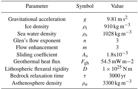
Table 1. Ice sheet–bedrock model parameter values.

Parameter Symbol Value

Gravitational acceleration g 9.81 m s2

Ice density ρi 910 kg m−3

Sea water density ρs 1028 kg m−3

Glen’s flow exponent n 3

Flow enhancement m 3

Sliding coefficient As 1.8x10−3

Geothermal heat flux Fgh 54.5 mW m−2

Lithospheric flexural rigidity D 1×1025N m

Bedrock relaxation time τ 3000 yr

Asthenosphere density ρa 3300 kg m−3

wherekandcpare the thermal diffusivity and specific heat capacity of the ice. The dissipation of energy due to ice defor-mation is represented by8. If the basal temperature reaches the pressure melting point, ice sliding over the bedrock is considered with a Weertman-type sliding law (Weertman, 1957).

The interaction with the the solid earth accounts for the bedrock response to the loading changes of the overlying ice. Changes in bedrock height modify the ice-sheet surface ele-vation and therefore the surface mass balance and ice thick-ness. We use two different formulations for the bedrock re-sponse. Firstly, the Earth is assumed to be a flat elastic litho-sphere (EL) resting over a viscous relaxed asthenolitho-sphere (RA). This is the so called ELRA model (Le Meur and Huy-brechts, 1996). According to the ELRA model, the bedrock responds with a downward deflectionwto the pressure ex-erted by a point loadq. The steady state displacementwis given by the following equation for a normalized distance x=r/Lr fromq(Le Meur and Huybrechts, 1996):

w (x)= qL 2 r

2π Dχ (x) , (4)

whereD is the flexural rigidity that allows the depression to extend beyond the point q where the load is located,χ is the zero order Kelvin function,r is the original distance from the load point, andLr is the radius of relative stiffness: Lr=(D/ρag)14. The elasticity of the lithosphere is assumed

to be linear; hence, the total deflection of the bedrock at some point can be calculated as the sum of the contribution of all neighboring points. While the lithosphere accounts for the shape of the deformation, the asthenosphere controls the time response. The rate of the vertical bedrock movement, ∂w_∂t is proportional to the deviation of the profile from the equilib-rium state,w−w0, and inversely proportional to the relax-ation timeτ (Le Meur and Huybrechts, 1996):

∂w ∂t =

−(w−w0)

τ . (5)

The second approach is a more complete physical approach, the Self Gravitational Viscoelastic (SGVE) model,

consist-ing of an elastic lithosphere, two viscoelastic mantle layers and an inviscid core (Le Meur and Huybrechts, 1996). In this model, the isostatic response to a loadLs(x, y, t )is given by Y (xi, yj, t )=

i+1i X i1=i−1i

j+1j X j1=j−1j

1x1y 0

Z

−Tm

G(1θ, t )Ls(x, y, t )dt , (6)

with1x 1ythe spatial resolution, G the Green’s functions, 1θthe angular distance between grid points, andTmthe pre-ceding 30 000 yr of ice-loading history. We use the SGVE model TABOO (Spada, 2003) in one experiment to compare and validate results from the default ELRA runs. The SGVE model is called every 500 yr by the ice-sheet model which is run on a 1-yr temporal resolution. Several tests with different time intervals have shown that it is justified to use the 500-yr interval for the SGVE model instead of the 100-yr interval used for the ELRA model. A viscosity of the upper layer of 1×1021Pa has been used and 2×1021Pa for the lower layer. To initialize the model, bedrock topography and ice thick-ness were taken from Bamber et al. (2001) with a spatial resolution of 20 km×20 km and the present-day reference SMB field and surface temperature from Ettema et al. (2009). The model runs with these initial values for 200 000 yr until a steady-state is reached.

3 Bedrock response to variations in surface mass balance

In order to analyze the solid earth motion in response to changes in ice thickness, we carried out a series of experi-ments, varying the forcing, the length of the simulation, and the way the solid earth is modeled.

3.1 Idealized last millennium experiment

In the first experiment we study the response of the bedrock to recent changes in the ice load. In order to do this, we mim-icked temperature variations over the last millennium by a sinusoidal function that oscillates around zero with an ampli-tude of 1 K and a period of 1000 yr. This approximation is in reasonable agreement with the reconstruction from Kobashi et al. (2009). The total length of the simulation is 60 kyr, al-though we focused the analysis on the last 3000 yr to remove the spin-up effect.

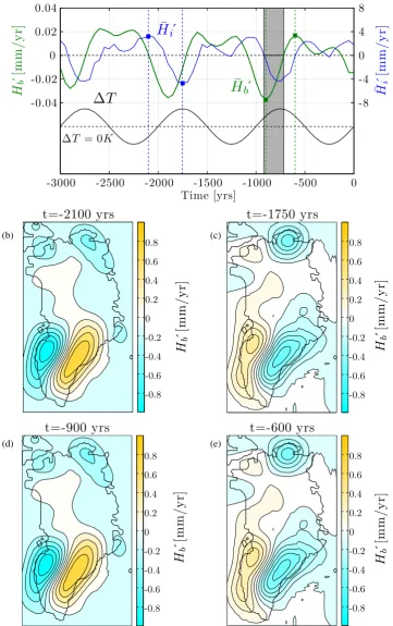
The evolution of the mean time derivatives of ice thick-ness (H¯_i0) and bedrock elevation (H¯_b0) are shown in Fig. 1a. Unless stated differently, bedrock changes are uplift rates and not geoid rates. The spatial averages are computed over all grid points in the domain excluding ocean. We plot the time derivatives to illustrate more precisely the phase lag between ice thickening (thinning) and bedrock subsidence (uplift). The temperature forcing (indicated without units by the black line as a reference) modifies the SMB, as well as

1266 M. Olaizola et al.: Bedrock adjustment patterns of the Greenland ice sheet

ice temperature and, as a consequence, ice viscosity. These changes result in ice thickness variations (blue line), and the bedrock responds with elevation changes (green line) that in turn modify surface elevation and therefore SMB. We con-sider PD (t=0 kyrs) as the initial time of the reference state that results from the initialization of the model. All temper-ature anomalies are relative to the PD conditions obtained from Ettema et al. (2009). Ice thins (negativeH¯_i0) during peri-ods when the temperature is above the PD value. The bedrock responds with uplift (positive values ofH¯_b0). During a time period of 200 yr, ice thinning and bedrock subsidence exist simultaneously, represented by the grey area in Fig. 1. The delay in the bedrock response to ice thickness changes, as well as its possible variations caused by a different forcing or by the way the solid earth is modeled, are important to con-sider as it might be an explanation for the results by W10. As the schematic experiment may depend on the values of the Earth parameters, we consider several time slices.

For this first experiment we obtain a maximum average bedrock subsidence ofH¯_b0= −0.04 mm yr−1att= −900 yr. This is the spatial average over the island and larger values can be found near the margins as shown in Fig. 1b, c, d and e, where we present the spatial patterns ofH_b0. Figures 1b and c (t= −2100 yr and t= −1750 yr) correspond to the time slices whereH¯_i0reaches its maximum and minimum values, respectively (blue points in Fig. 1a). In Fig. 1d and e (t= −900 yr andt= −600 yr),H¯_b0is respectively at its minimum and at its maximum (green points in Fig. 1a).

The pattern ofH_b0 att= −2100 yr (Fig. 1b) is character-ized by bedrock subsidence (blue colors) along the western margin. This is an area of large ablation where the SMB in-creases as a consequence of lower temperatures. As a result, ice thickens and the bedrock subsides, although with a de-lay. In the southeast, the main accumulation area, a decrease in SMB due to lower temperatures (reflecting less accumula-tion) yields ice thinning and therefore bedrock uplift (yellow to red colors).

When the temperature increases att= −1750 yr, the op-posite occurs. The bedrock subsides in the accumulation area located in the southeast where the positive SMB is the domi-nant factor. In these areas an increase in temperature leads to an increase in SMB (reflecting a higher precipitation). Over the rest of the island, the temperature increase is followed by a decrease in SMB (higher ablation), which results in less ice volume (minimum value ofH¯_i0) and bedrock uplift.

At t= −900 yr the pattern is similar to the one at t= −2100 yr. Bedrock subsidence is observed along the west-ern margin since the bedrock is still reacting to past changes when the temperature was lower. This results in a higher SMB (reduced ablation) and thus ice thickening. In the south-east, SMB decreases, ice thins, and bedrock uplifts.

Att= −600 yr,H¯_b0reaches its maximum and the pattern is similar to the one att= −1750 yr, characterized by bedrock uplift in the southwest and bedrock subsidence in the south-east.

In all cases, the imprint is most pronounced in the southern half of the island. Additionally, the signal alternates period-ically between bedrock subsidence and uplift being stronger along the margin. This is due to the spatial pattern of sur-face mass balance with the main ablation area located in the southwest and a high accumulation region in the southeast. As such, the pattern does not depend much on the details of the mass balance formulation. Nevertheless the absolute value may still depends on processes with longer time scales as well as on the specific choice of Earth parameters. For this reason longer time scales are consider in the following experiment.

3.2 Holocene and last deglaciation, schematic experiment

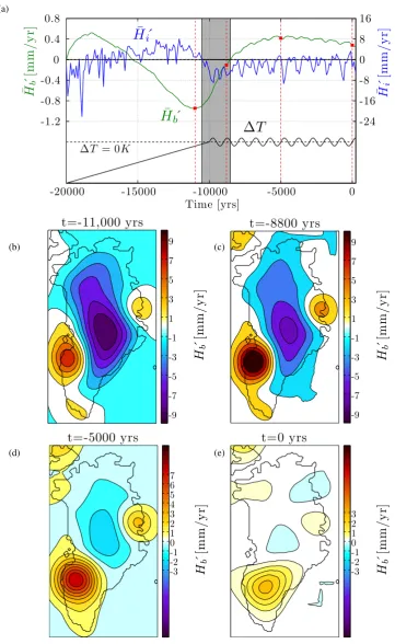
Since bedrock response shows a lag to changes in ice thick-ness, it is also necessary to study the effect of the last glacial cycle on the magnitude of the lag, which yields a different thermal condition of the ice sheet affecting the dynamical re-sponse and hence the bedrock rere-sponse. In this section we present the results of a schematic experiment consisting of different forcing periods. First a steady-state run is performed with PD temperatures lowered by 10 K for 100 kyr, simulat-ing a glacial area. After this, the model is forced with a lin-early increasing temperature which reaches the PD value at 10 kyr, corresponding to a fast transition to the Holocene. Fi-nally, the temperature oscillates around its PD value as a sine function with an amplitude of 1 K and a period of 1000 yr for another 10 kyr, similar to the previous experiment. In Fig. 2a, the forcing is illustrated as a black line, the blue line shows changes in ice thickness and the bedrock response is shown in green.

During the first 3000 yr (between the years−20 000 and −17 000), the temperature increase results in a lower SMB and hence ice thinning. Hereafter, warmer conditions (be-tween −4 K and PD) also increase accumulation (positive SMB), which becomes the dominant effect during this pe-riod. Therefore, ice starts to thicken (positive values ofH¯_i0) around the year−17 000. Att=10500 yr (left side of the grey rectangle in Fig. 2a),H¯_i0 changes sign to negative val-ues, meaning that ice thins due to the continuing increasing temperature. The bedrock reacts to this ice load reduction with an uplift, although with a delay of 1990 yr, indicated by the grey rectangle in Fig. 2a. Hence, there is again a period where ice thinning coincides with bedrock subsidence.

M. Olaizola et al.: Bedrock adjustment patterns of the Greenland ice sheet_{M. Olaizola et al.: Bedrock response to mass changes for the GrIS} 1267 ₉

∆

T

∆T = 0K

¯

Hb

´

¯

Hi

´

Time [yrs]

¯

H

´

[m

m

/

y

r]

-0.04 -0.02 0 0.02 0.04

¯

H

´

[m

m

/

y

r]

-3000 -2500 -2000 -1500 -1000 -500 0

-8 -4 0 4 8

t=-2100 yrs

H

´

[m

m

/

y

r]

-0.8 -0.6 -0.4 -0.2 0 0.2 0.4 0.6 0.8

t=-1750 yrs

H

´

[m

m

/

y

r]

-0.8 -0.6 -0.4 -0.2 0 0.2 0.4 0.6 0.8

t=-900 yrs

H

´

[m

m

/

y

r]

-0.8 -0.6 -0.4 -0.2 0 0.2 0.4 0.6 0.8

t=-600 yrs

H

´

[m

m

/

y

r]

-0.8 -0.6 -0.4 -0.2 0 0.2 0.4 0.6 0.8

(a)

(b) (c)

(d) (e)

Fig. 1. (a) Time evolution of the spatial averageH¯b0(green line) andH¯i0(blue line) for a forcing (black line) that schematically simulates

temperature variations during the last 3000 years of the Holocene. The grey rectangle illustrates the 200 yr delay between the start of ice thinning (H¯i0 transition of positive to negative values) and onset of the bedrock response by uplift (H¯b0 transition to negative values). (b-e)

Spatial patterns of bedrock elevation changes for time slices where (b)H¯i0reaches its maximum value; (c)H¯i0is at its a minimum; (d)H¯b0is

at its minimum; (e)H¯b0is at its maximum. Fig. 1. (a) Time evolution of the spatial average_H¯0

b(green line) andH¯

0

i (blue line) for a forcing (black line) that schematically simulates

temperature variations during the last 3000 yr of the Holocene. The grey rectangle illustrates the 200 yr delay between the start of ice thinning

(_H¯0

i transition of positive to negative values) and onset of the bedrock response by uplift (H¯

0

btransition to negative values). (b–e) Spatial

patterns of bedrock elevation changes for time slices where (b)H¯_i0reaches its maximum value, (c)H¯_i0is at its minimum, (d)H¯_b0 is at its

minimum, and (e)_H¯0

bis at its maximum.

1268 M. Olaizola et al.: Bedrock adjustment patterns of the Greenland ice sheet 10 M. Olaizola et al.: Bedrock response to mass changes for the GrIS

∆

T

¯

H

´

¯

Hi

´

∆T = 0K

Time [yrs]

¯

H

´

[m

m

/

y

r]

-1.2 -0.8 -0.4 0 0.4 0.8

¯

H

´

[m

m

/

y

r]

-20000 -15000 -10000 -5000 0

-24 -16 -8 0 8 16

t=-11,000 yrs

t=-8800 yrs

H

´

[m

m

/

y

r]

-9 -7 -5 -3 -1 1 3 5 7 9

H

´

[m

m

/

y

r]

-9 -7 -5 -3 -1 1 3 5 7 9

t=-5000 yrs

H

´

[m

m

/

y

r]

-3 -2 -1 0 1 2 3 4 5 6 7

t=0 yrs

H

´

[m

m

/

y

r]

-3 -2 -1 0 1 2 3

(a)

(b) (c)

(d) (e)

Fig. 2.(a) Time evolution of the spatial averageH¯b0andH¯

0

ifor a forcing that simulates the last deglaciation and 10 000 years of the Holocene.

Once the ice thins (negative values ofH¯i0), the bedrock reacts with uplift with a lag of 1,990 yrs. The grey area shows a period when thinning

of the ice is present as well as bedrock subsidence. (b-e) Spatial patterns of bedrock elevation changes for the selected red squares in (a) for: (b) the maximum subsidence; (c) a moment when ice thinning and bedrock subsidence exist simultaneously; (d) a moment whenH¯b0is

positive (bedrock uplift); (e) PD conditions, characterized by an average bedrock uplift.

Fig. 2. (a) Time evolution of the spatial averageH¯_b0 andH¯_i0for a forcing that simulates the last deglaciation and 10 000 yr of the Holocene.

Once the ice thins (negative values ofH¯_i0), the bedrock reacts with uplift with a lag of 1990 yr. The grey area shows a period when thinning

of the ice is present as well as bedrock subsidence. (b–e) Spatial patterns of bedrock elevation changes for the selected red squares in (a)

for: (b) the maximum subsidence, (c) a moment when ice thinning and bedrock subsidence exist simultaneously, (d) a moment whenH¯_b0is

M. Olaizola et al.: Bedrock adjustment patterns of the Greenland ice sheet 1269

d and e. Att= −8800 yr, while the area of central subsi-dence is reduced, the uplift region located in the southwest becomes larger and more extended than att= −11000 yr. At t= −5000 yr, the amplitude of the signal (uplift as well as subsidence) decreases. The area of subsidence in the center is strongly reduced, which is reflected inH¯_b0which increases to 0.4 mm yr−1. For PD conditions (t=0), the bedrock sub-sidence in the center almost vanishes and the pattern is char-acterized by an average upliftH¯_b0=0.3 mm yr−1. In compar-ison with the millennium experiment (Sect. 3.1), we note a stronger signal as well as a shift of the dipole structure in the northern direction.

Since different physical formulations of the solid earth might have a strong impact on the values ofH¯_b0, we used the more sophisticated Self Gravitational Viscoelastic (SGVE) model in addition to the ELRA model to compare and val-idate the previous results. Hence, we repeat the experiment with the same forcing but now with an SGVE model for the bedrock.

Figure 3a shows the values ofH¯_i0(left plot) andH¯_b0 (right plot) for the two models, showing qualitative similar re-sults. The general behavior of theH_b0 patterns (Fig. 2 and 3) are similar as well. As a result of the last glaciation, there is a strong bedrock subsidence in the center that van-ishes with time. For the SGVE model, the minimum value of

¯

H_b0= −0.6 mm yr−1occurs att= −11,000 yr (similar to the ELRA model), and then starts to relax. Att= −8,800 yr, the value increases to _H¯0

b= −0.1 mm yr

−1_{. At t= −5,000 yr,} an average uplift is observed, H¯_b0=0.2 mm yr−1 with the same value obtained for PD. The largest differences in the patterns for the two models occur in north Greenland. Bedrock uplift is found in this region for the last three se-lected time slices in the SGVE model, while with the ELRA model, there is nearly no bedrock movement in that area. Re-garding the PD pattern for central Greenland, results from the two models display bedrock subsidence. Nevertheless, a closer look shows that the center of subsidence in the SGVE model is somewhat shifted in the southwestern direction. This is caused by the stronger uplift in the north, and as a consequence the eastern margins in the SGVE model expe-rience a larger subsidence. Moreover, the lag of the bedrock response increases with respect to the ELRA model to a value of 2400 yr. Obviously the phasing and the magnitude of the results will change slightly for different settings of Earth pa-rameters, but unless spatially varying Earth properties are used, there is no reason to assume significant changes in the dipole patterns.

3.3 Holocene and last deglaciation, ice core data

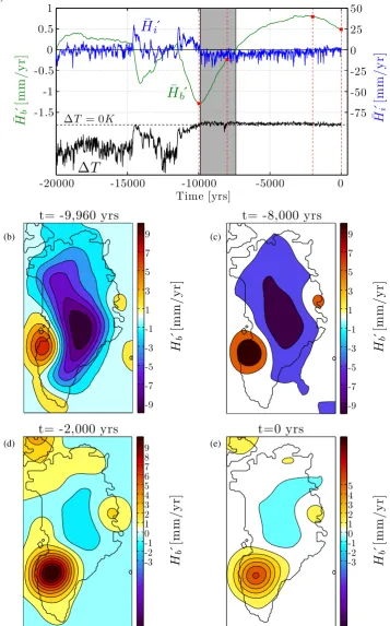
In order to study the bedrock response to present-day changes in ice thickness in a more realistic way than in the previous schematic experiments, we used a temperature record from an ice core as a forcing, based on the GRIP δ18Oconverted into a surface temperature record following

Johnsen et al. (1995). Results as obtained using the ELRA model are shown in Fig. 4a. Between the years−20 000 and −10 000,1T remains negative, which allows ice thicken-ing, especially when the temperature strongly increases, (as for t= −14500 yr) because a warmer climate is character-ized by higher accumulation rates, which are reflected in the SMB. In fact, for very cold periods, (from −20 000 to −15 000 yr), SMB is reduced and this yields ice thinning and bedrock uplift. During the Holocene (fromt= −10000 yr to PD),1T oscillates around zero. This results in ice thinning from t= −10200 yr (indicated by the left side of the grey rectangle in Fig. 4a). Negative values of H¯_i0 persist during the Holocene with a few short periods of ice thickening. The ice load reduction causes bedrock uplift (t= −8400 yr, right side of the grey rectangle) with a lag of 2800 yr.

In Fig. 4b, c and d, we show the patterns of bedrock eleva-tion changes for the selected red points in Fig. 4a. The over-all evolution of the pattern is similar to the one presented in the previous section. The bedrock subsidence present in the center diminishes and areas of bedrock uplift appear along the margins, although in this case, the strength of the imprint is larger compared to the previous experiments. The maxi-mum bedrock subsidence is att= −9980 yr, reaching a value of H¯_b0= −1.3 mm yr−1. Att= −8000 yr, the bedrock sub-sidence is reduced toH¯_b0= −0.2 mm yr−1. Later on, at t= −2000 yr, the maximum bedrock uplift occurs with a value

¯

H_b0=0.8 mm yr−1_{, which decreases to H}¯0

b=0.5 mm yr −1

for PD.

4 Conclusions

To analyze the interaction between variations in ice load-ing and the response in bedrock durload-ing the Holocene, a se-ries of experiments were carried out as presented in Sect. 3. In Sect. 3.1 the temperature along the last millennium is schematically represented by a 1 K-amplitude sine function with a period of 1000 yr. In this experiment we found a lag of the bedrock response of 200 yr, where the precise lag de-pends slightly on parameter settings. In reality, temperature variations are more complex than the sinusoidal function used in the experiment. Nevertheless, it suggests that we can generate cases where the bedrock is still reacting to changes in ice thickness that happened 200 yr ago. This is compati-ble with the LIA that occurred between 1400 and 1900. The time lag of the bedrock response allows for a situation of si-multaneous ice thinning (due to an increase in temperature or negative MB) and bedrock subsidence, as suggested by W10. We obtained similar values for this lag varying the ampli-tude (up to 5 K) as well as varying the bedrock relaxation time τ to 5000 yr, which was fixed to 3000 yr in the ex-periments presented in this paper. In the ELRA model, the long-term response of the bedrock is controlled by the as-thenosphere, being inversely proportional to the relaxation time. The numerical values ofτ are based on assumptions

1270 M. Olaizola et al.: Bedrock adjustment patterns of the Greenland ice sheet M. Olaizola et al.: Bedrock response to mass changes for the GrIS 11

SGVE

ELRA

Time [kyr] ¯_H´b

[m

m

/

y

r]

-20 -15 -10 -5 0

-0.8 -0.4 0 0.4 0.8

SGVE ELRA

Time [kyr]

¯_H´i

[m

m

/

y

r]

-20 -15 -10 -5 0

-18 -14 -10 -6 -2 2 6

t=-11,000 yrs

H

´

[m

m

/

y

r]

-9 -7 -5 -3 -1 1 3 5 7 9

t=-8800 yrs

H

´

[m

m

/

y

r]

-9 -7 -5 -3 -1 1 3 5 7 9

t=-5000 yrs

t=0 yrs

H

´

[m

m

/

y

r]

-3 -2 -1 0 1 2 3 4 5 6 7

H

´

[m

m

/

y

r]

-3 -2 -1 0 1 2 3

(a)

(b) (c)

(d) (e)

Fig. 3.(a) Comparison between values ofH¯i0andH¯

0

bobtained with the ELRA and SGVE models showing qualitatively similar results. (b-e)

Patterns ofHb0with the SGVE model for the selected time points in Fig. 2a for (b) the maximum subsidence; (c) and (d) moments when the

strong subsidence at the center starts to fade; (e) present-day conditions, characterized by an average bedrock uplift.)

Fig. 3. (a) Comparison between values ofH¯i0andH¯b0obtained with the ELRA and SGVE models showing qualitatively similar results. (b–e)

Patterns ofH_b0with the SGVE model for the selected time points in Fig. 2a for (b) the maximum subsidence, (c) and (d) moments when the

M. Olaizola et al.: Bedrock adjustment patterns of the Greenland ice sheet 1271 12 M. Olaizola et al.: Bedrock response to mass changes for the GrIS

∆T = 0K

∆

T

¯

H

´

¯

Hi

´

Time [yrs]

¯

H

´

[m

m

/

y

r]

-1.5 -1 -0.5 0 0.5 1

¯

H

´

[m

m

/

y

r]

-20000 -15000 -10000 -5000 0

-75 -50 -25 0 25 50

t= -9,960 yrs

H

´

[m

m

/

y

r]

-9 -7 -5 -3 -1 1 3 5 7 9

t= -8,000 yrs

H

´

[m

m

/

y

r]

-9 -7 -5 -3 -1 1 3 5 7 9

t= -2,000 yrs

H

´

[m

m

/

y

r]

-3 -2 -1 0 1 2 3 4 5 6 7 8 9

t=0 yrs

H

´

[m

m

/

y

r]

-3 -2 -1 0 1 2 3 4 5

(a)

(b) (c)

(d) (e)

Fig. 4.a) Time evolution of the spatial averageH¯b0(blue line) andH¯

0

i(green line) for a temperature forcing from ice core data (black line).

The grey rectangle shows the lag of the bedrock response of 2800 yrs. (b-e) Spatial patterns of bedrock elevation for the selected red points for( b) the maximum subsidence; (c) a moment when ice thinning and bedrock subsidence exist simultaneously; (d) a moment close to the maximum uplift; (e) present-day conditions, characterized by an average bedrock uplift.

Fig. 4. (a) Time evolution of the spatial averageH¯_b0 (blue line) andH¯_i0(green line) for a temperature forcing from ice core data (black line). The grey rectangle shows the lag of the bedrock response of 2800 yr. (b–e) Spatial patterns of bedrock elevation for the selected red points for ( b) the maximum subsidence, (c) a moment when ice thinning and bedrock subsidence exist simultaneously, (d) a moment close to the maximum uplift, and (e) present-day conditions, characterized by an average bedrock uplift.

1272 M. Olaizola et al.: Bedrock adjustment patterns of the Greenland ice sheet

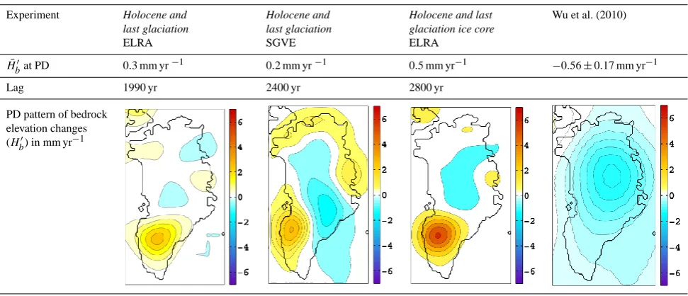
Table 2. Comparison of lag values,H¯_b0 and the PD bedrock patterns obtained in this study and the geodic pattern reported by and Wu et al. (2010). The values of bedrock changes corresponding to the experiments presented in this paper are uplift rates while the ones by W10 are geodic rates.

Experiment Holocene and Holocene and Holocene and last Wu et al. (2010)

last glaciation last glaciation glaciation ice core

ELRA SGVE ELRA

¯

H_b0at PD 0.3 mm yr−1 0.2 mm yr−1 0.5 mm yr−1 −0.56±0.17 mm yr−1

Lag 1990 yr 2400 yr 2800 yr

PD pattern of bedrock elevation changes

(H_b0) in mm yr−1

about the viscosity of the Earth’s interior. Moreover, about half of the error in the models used to calculate GIA trends is due to the lack of information on the Earth’s viscosity pro-file (Velicogna and Wahr, 2006). Here we only mimic that by variations inτ, which introduce a maximum difference in the values of the lag of 20 % (in case of a period in the forcing of 10 000 yr). Therefore, an error of 20 % can be assigned to the magnitude of the lag. This may also be achieved by variations in Earth parameters.

The maximum average bedrock subsidence found in the long time scale experiment isH¯_b0= −0.4 mm yr−1, increas-ing up to−1 mm yr−1 near the margins. Although we can obtain a result for which the order of magnitude of the sub-sidence is in accordance with the one reported by W10, the spatial pattern of bedrock changes differs considerably. We observed the highest values in the lower half of the island and not in the center. Moreover, oscillations between subsi-dence and uplift in the southwest and southeast occur instead of an overall subsidence, due to the fact that in those areas the largest ice changes have taken place. In fact, assuming that the entire ice sheet has undergone a spatially uniform climatic history, any realistic mass balance forcing will lead to a stronger response over the margin than in the center, as ice thickness changes are larger near the margin. This is ir-respective of the fact that we consider local bedrock changes while W10 considered geoid changes.

If we want to explain the pattern by W10 by a recent mass change (applied some 100 yr ago, so an elastic response), a disk ice load would be needed with 5 degrees diameter and a thickness of 300 m located in central Greenland. From a mass balance perspective, this is not realistic and indicates that the observed geoid changes by W10 seem very peculiar.

Nevertheless, it should be noted that this first experiment is a schematic way to approximate the present-day condi-tions of the GrIS. A limitation of this experiment is the steady state initial condition. Therefore a second experiment was carried out that includes the last (de)glaciation preced-ing the Holocene temperature variations (Sect. 3.2). Also in this case, a time slice exists where bedrock subsidence and ice thinning coincides. Furthermore, the spatial pattern of bedrock elevation shows a strong subsidence in the center just after the deglaciation started, although in combination with uplift in the west, which is an ablation area. The in-tensity and the extension of the central subsidence decreases over time until it almost vanishes. For PD conditions, the pattern of the bedrock elevation shows a strong uplift in the south and northwest, up to 1 mm yr−1, in combination with a subsidence of−0.05 mm yr−1in the center. The average bedrock uplift for PD is_H¯0

b=0.3 mm yr

−1_{. A similar pattern} was obtained with the ICE5G model, as reported by Peltier (2004), where subsidence is present in a small area in the northern part of Greenland and in a band around the center-southeast, while uplifting occurs in the north and southwest with an average bedrock uplift of 0.1±0.35 mm yr−1 for PD. This model has been used to correct GRACE data by GIA trend in several studies (e.g. Velicogna and Wahr, 2006; Velicogna, 2009) which reported a mass balance loss around twice the estimate of W10.

M. Olaizola et al.: Bedrock adjustment patterns of the Greenland ice sheet 1273

strong subsidence in the center resulting from an accumula-tion increase since the last glaciaaccumula-tion that fades with time. Although, the resulting patterns for the PD show different characteristics with the SGVE model: a more pronounced uplift is present in the north; the central subsidence is over a more extended area; and the uplift in the margin is stronger. This would be a realistic bedrock response according to the changes in ice thickness as reported by W10 and Thomas et al. (2006) with thickening of the ice in the elevated areas of the GrIS and ice thinning at lower elevations. We conclude that qualitatively similar results can be obtained with the two models, and due to the computationally less expensive simu-lations, we choose the ELRA model for the last experiment. We definitely do not want to claim that different Earth pa-rameter settings in the SGVE are not affecting the magnitude of the signal, but the dipole structure that characterizes the response will remain. This is furthermore confirmed by the experiments of Simpson et al. (2011), who also mainly find dipole structures coupled to the areas with more ice mass changes.

To perform a more realistic experiment, we used a tem-perature record based on ice core data as a forcing with again qualitatively similar results (Sect. 3.3). The lag of the bedrock response to ice thickness changes in the last deglaciation is 2800 yr, and for the PD we found a positive value ofH¯_b0=0.5 mm yr−1. In this case the H¯_b0 pattern for PD is also similar to the one reported by Peltier (2004).

In Table 2, we show a summary of the results of the ice sheet–bedrock experiments presented in this paper.

In all the experiments we applied the novel SMB gradi-ent parameterization (Helsen et al., 2012) where the time evolution of the SMB is based on changes in surface ele-vation rather than via a constant lapse rate, as is the case for the PDD method often used in ice-sheet models. The SMB model formulation has an influence on the results. This is clear in the first experiment (Sect. 3.1) where an alternation between bedrock subsidence and uplift in the southwest and southeast of Greenland was found. This is due to the SMB which is characterized by strong ablation in the southwest and an accumulation area in the southeast. Table 2 clearly shows a different sign and pattern between the results by W10 and our modeling results which cannot be explained by the difference in geoid rate and uplift rates.

A limitation of the applied model is the lack of detail with respect to outlet glaciers, particularly in the southeast. Those outlet glaciers are partly in different regions, so the ice thick-ness change pattern may be somewhat different from what we find, but the largest changes will always take place in the marginal zones and would yield qualitatively similar results for the bedrock response pattern.

In all the experiments we found a lag of the bedrock re-sponse to ice thickness changes not higher than 3000 yr. This implies that a bedrock subsidence, caused by a delay in the bedrock response that is still reacting to a net past ice ac-cumulation during the glacial period, is not possible for PD

conditions (after more than 10 000 yr of the end of the last glacial cycle). In fact, the bedrock is already adjusted to the ice load reduction and an average bedrock uplift is present in Greenland. Therefore, we conclude that for present day, a bedrock subsidence with a maximum over the central parts of Greenland as reported by W10 cannot be explained by past mass changes in the surface mass balance as the authors sug-gested, not by the deglaciation, and also not by changes since the Little Ice Age. Bedrock change patterns are spatially re-stricted to the areas where ice mass changes are largest. This undermines the result of a mass loss of half of the values re-ported in earlier studies.

Acknowledgements. We would like to thank Thomas Reerink

for his role in the development of the ANICE model. Financial support was provided by the Netherlands Organization of Scientific Research (NWO) in the framework of the Netherlands Polar Programme (NPP). This work contributes to the Knowledge for Climate (KvK) program in the Netherlands. We thank G. Spada and E. v. d. Linden for help with the SGVE code and Paolo Stocchi for the interpretation of the SGVE results. We thank Shawn Marshall for meticulous editing of the manuscript.

Edited by: S. Marshall

References

Bamber, J. L., Layberry, R. L., and Gogineni, S. P.: A new ice thick-ness and bed data set for the Greenland ice sheet 1. measurement, data reduction, and errors, J. Geophys. Res., 106, 33773–33780, 2001.

Ettema, J., Van den Broeke, M. R., van Meijgaard, E., van de Berg, W. J., Bamber, J. L., Box, J. E., and Bales, R. C.: Higher sur-face mass balance of the Greenland ice sheet revealed by high-resolution climate modeling, Geophys. Res. Lett., 36, L12501, doi:10.1029/2009GL038110, 2009.

Fleming, K., Martinec, Z., and Hagedoorn, J.: Geoid displace-ment about Greenland resulting from past and presentday mass changes in the Greenland Ice Sheet, Geophys. Res. Lett., 31, L06617, doi:10.1029/2004GL019469, 2004.

Helsen, M. M., van de Wal, R. S. W., van den Broeke, M. R., van de Berg, W. J., and Oerlemans, J.: Coupling of climate models and ice sheet models by surface mass balance gradients: appli-cation to the Greenland Ice Sheet, The Cryosphere, 6, 255–272, doi:10.5194/tc-6-255-2012, 2012.

Hutter, K.: Theoretical glaciology: material science of ice and the mechanics of glaciers and ice sheets, Reidel Publ. Co., Dor-drecht., 548 pp., 1983.

Huybrechts, P. and de Wolde, J. R.: The dynamic response of the Greenland and Antarctic ice sheets to multiple century climatic warming, J. Climate, 12, 2169–2188, 1999.

Huybrechts, P. and Le Meur, E.: Predicted present day evolution patterns of ice thickness and bedrock elevation over Greenland and Antarctica, Polar Res., 18, 299–306, 1999.

Johnsen, S. J., Dahl-Jensen, D., Dansgaard, W., and Gundestrup, N.: Greenland palaeotemperatures derived from GRIP bore hole

1274 M. Olaizola et al.: Bedrock adjustment patterns of the Greenland ice sheet

temperature and ice core isotope profiles, Tellus, 47B, 624–629, 1995.

Kobashi, T., Severinghaus, J. P., Barnola, J. M., Kawamura, K., Carter, T., and Nakaegawa, T.: Persistent multi-decadal Green-land temperature fluctuation through the last millennium, Cli-mate Change, 100, 733–756, 2009.

Le Meur, E. and Huybrechts, P.: A comparison of different ways of dealing with isostasy: examples from modelling the antarctic ice sheet during the last glacial cycle, Ann. Glaciol., 23, 309–317, 1996.

Lemke, P., Ren, J., Alley, R. B., Allison, I., Carrasco, J., Flato, G., Fujii, Y., Kaser, G., Mote, P., Thomas, R. H., and Zhang, T.: Observations: Changes in Snow, Ice and Frozen Ground, in: Climate Change 2007: The Physical Science Basis. Contribution of Working Group I to the Fourth Assessment Report of the In-tergovernmental Panel on Climate Change, edited by: Solomon, S., Qin, D., Manning, M., Chen, Z., Marquis, M., Averyt, K. B., Tignor, M. and Miller, H. L., Cambridge University Press, Cam-bridge, United Kingdom and New York, NY, USA, 337–383, 2007.

Peltier, W. R.: Global Glacial Isostasy and the Surface of the Ice-Age Earth: The Ice-5G (VM2) Model and GRACE, Ann. Ren. Earth Planet, 32, 111–149, 2004.

Rignot, E. G., Bamber, J. L., van den Broeke, M. R., Davis, C., Li, Y., van de Berg, W., and van Meijgaard, E.: Recent Antarctic mass loss from radar interferometry and regional climate mod-elling, Nature Geosci., 2, 106–110, 2008.

Simpson, M., Wake, L., Milne, G., and Huybrechts, P.: The influ-ence of decadal to millennial scale ice mass changes on present day vertical land motion in Greenland: Implications for the inter-pretation of GPS observations, J. Geophys. Res., 116, B02406, doi:10.1029/2010JB007776, 2011.

Spada, G.: The theory behind TABOO. Samizdat Press, Golden-White River Junction, 108 pp., 2003.

Tarasov, L. and Peltier, W.: Greenland glacial history and local geo-dynamic consequences, Geophys. J. Int., 150, 198–229, 2002. Tedesco, M., Fettweis, X., van den Broeke, M. R., van de Wal, R.

S. W., Smeets, C. J. P., van de Berg, W. J., Serreze, M. C., and E., B. J.: The role of albedo and accumulation in the 2010 melting record in Greenland, Environ. Res. Lett., 6, 1–6, 10.1088/1748-9326/6/1/014005, 2011.

Thomas, R., Frederick, E., Krabill, W., Manizade, S., and Martin, C.: Progressive increase in ice loss from Greenland, Geophys. Res. Lett., 33, L10503, doi:10.1029/2006GL026075, 2006. van de Wal, R. S. W.: Mass-balance modelling of the greenland

ice sheet: a comparison of an energy-balance and a degree-day model, Ann. Glaciol., 23, 36–45, 1996.

van de Wal, R. S. W.: The importance of thermodynamics for mod-eling the volume of the greenland ice sheet, J. Geophys. Res., 104, 3889–3898, 1999.

van den Broeke, M., Bamber, J., Ettema, J., Rignot, E., Schrama, E., van de Berg, W., Meijgaard, E., Velicogna, I., and Wouters, B.: Partitioning Recent Greenland Mass Loss, Science, 326, 984– 986, 2009.

van der Veen, C. J.: Fundamentals of glacier dynamics, AA Balkema, Rotterdam, 462 pp., 1999.

Velicogna, I.: Increasing rates of ice mass loss from the Green-land and Antarctic ice sheets revealed by GRACE, Geophys. Res. Lett., 36, L19503, doi:10.1029/2009GL040222, 2009.

Velicogna, I. and Wahr, J.: Acceleration of Greenland ice mass loss in spring 2004, Nature, 443, 329–331, 2006.

Weertman, J.: On the sliding of glaciers, J. Glaciol., 3, 33-38, 1957 Wouters, B., Chambers, D., and Schrama, E.: GRACE observes small-scale mass loss in Greenland, Geophys. Res. Lett., 35, L20501, doi:10.1029/2008GL034816, 2008.