RESEARCH
A safe and complete algorithm
for metagenomic assembly
Nidia Obscura Acosta, Veli Mäkinen and Alexandru I. Tomescu
*Abstract
Background: Reconstructing the genome of a species from short fragments is one of the oldest bioinformat-ics problems. Metagenomic assembly is a variant of the problem asking to reconstruct the circular genomes of all bacterial species present in a sequencing sample. This problem can be naturally formulated as finding a collection of circular walks of a directed graph G that together cover all nodes, or edges, of G.
Approach: We address this problem with the “safe and complete” framework of Tomescu and Medvedev (Research in computational Molecular biology—20th annual conference, RECOMB 9649:152–163, 2016). An algorithm is called safe if it returns only those walks (also called safe) that appear as subwalk in all metagenomic assembly solutions for G. A safe algorithm is called complete if it returns all safe walks of G.
Results: We give graph-theoretic characterizations of the safe walks of G, and a safe and complete algorithm finding all safe walks of G. In the node-covering case, our algorithm runs in time O(m2+n3), and in the edge-covering case
it runs in time O(m2n); n and m denote the number of nodes and edges, respectively, of G. This algorithm constitutes
the first theoretical tight upper bound on what can be safely assembled from metagenomic reads using this problem formulation.
Keywords: Genome assembly, Contig assembly, Metagenomics, Graph algorithm, Circular walk
© The Author(s) 2018. This article is distributed under the terms of the Creative Commons Attribution 4.0 International License (http://creativecommons.org/licenses/by/4.0/), which permits unrestricted use, distribution, and reproduction in any medium, provided you give appropriate credit to the original author(s) and the source, provide a link to the Creative Commons license, and indicate if changes were made. The Creative Commons Public Domain Dedication waiver (http://creativecommons.org/ publicdomain/zero/1.0/) applies to the data made available in this article, unless otherwise stated.
Background
One of the oldest bioinformatics problems is to recon-struct the genome of an individual from short fragments sequenced from it, called reads (see [1–3] for some genome assembly surveys). Its most common mathemati-cal formulations refer to an assembly (directed) graph built from the reads, such as a string graph [4, 5] or a de Bruijn graph [6, 7]. The nodes of such a graph are labeled with reads, or with sub-strings of the reads.1 Standard
assembly problem formulations require to find e.g., a node-covering circular walk in this graph [8], an edge-covering circular walk [8–11],2 a Hamiltonian cycle [12,
13] or an Eulerian cycle [7]. 1 We refer the reader to [4–7] for definitions of string graphs and de Bruijn
graphs, as they are not essential to this paper.
2 Node- and edge-covering walks usually refer to node- and edge-centric de Bruijn graphs, respectively. In the node-centric de Buijn graph, all k-mers in the reads are nodes of the graph, and edges are added between all k-mers that have a suffix-prefix overlap of length k−1. In the edge-centric de Bruijn
graph, it is further required that the k+1-mer obtained by overlapping the
two k-mers of an edge also appears in the reads. Thus for edge-centric de Bruijn graphs it reasonable to require that the walk covers all edges, because all edges also appear in the reads; this may not be the case for node-centric de Bruijn graphs.
Real assembly graphs have however many possible solutions, due mainly to long repeated sub-strings of the genome. Thus, assembly programs used in prac-tice, e.g., [5, 14–18], output only (partial) strings that are promised to occur in all solutions to the assembly prob-lem. Following the terminology of [19], we will refer to such a partial output as a safe solution to an assembly problem; an algorithm outputting all safe solutions will be called complete. Even though practical assemblers incor-porate various heuristics, they do have safe solutions at
Open Access
*Correspondence: [email protected]
their core. Improving these can improve practical assem-bly results, and ultimately characterizing all safe solutions to an assembly problem formulation gives a tight upper bound on what can be reliably assembled from the reads.
We will assume here that the genome to be assembled is a node or edge-covering circular walk of the input graph, since Hamiltonian or Eulerian cycle formulations unrealistically assume that each position of the genome is sequenced exactly the same number of times. The quest for safe solutions for this assembly problem formulation has a long history. Its beginnings can be traced to [20], which assembled the paths whose internal nodes have in-degree and out-degree equal to one. The method [7] assembled those paths whose internal nodes have out-degree equal to one, with no restriction on their in-degree. Other strategies such as [9, 21, 22] are based on iteratively reducing the assembly graph, for example by contracting edges whose target has in-degree equal to one. In [19], Tomescu and Medvedev found the first safe and complete algorithms for this problem, by giving a graph-theoretic characterization of all walks of a graph that are common to all of its node or edge-covering cir-cular walks. The algorithm for finding them, though proven to work in polynomial time, launches an exhaus-tive visit of all walks starting at each edge, and extend-ing each walk as long as it satisfies the graph-theoretic characterization.
The present paper is motivated by metagenomic sequencing [23, 24], namely the application of genomic sequencing to environment samples, such as soils, oceans, or parts of the human body. For example, metagenomic sequencing helped discover connections between bacte-ria in the human gut and bowel diseases [25, 26] or obe-sity [27]. A metagenomic sample contains reads from all the circular bacterial genomes present in it.
Because of the multiple genomes present in the sample, one can no longer formulate a solution for the metagen-omic assembly problem as a single circular walk cover-ing all the nodes or edges. A natural analog is to find a collection of circular walks of an assembly graph (i.e., the circular bacterial genomes), which together cover all the nodes, or edges, of the graph (i.e., they together explain
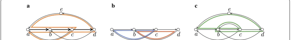
all the reads). In general, we do not know how many bac-terial species are in the sample, so we cannot place any bound on the number of circular walks. Hence, in our above formulation they can be any arbitrary number. See the next section for formal definitions, and Fig. 1 for a simple example.
It can be easily verified that the walks from [7, 9, 20– 22]—which are safe for single circular covering walks— are also safe for this metagenomic problem formulation. However, even though many practical metagenomic assemblers exist, e.g., [28–34], no other safe solutions are known for this problem formulation.
In this paper we solve this problem, by giving a graph-theoretic characterization of all walks w of a graph G such that for any metagenomic assembly solution R of G, w is a sub-walk of some circular walk in R. As opposed to the exhaustive search strategy from [19], in this paper we devise a new type of safe and complete algorithm for which we can tightly bound the running time. This works by outputting one solution to the metagenomic assembly problem, and then marking all its sub-walks that satisfy our characterization. The algorithm for the node-covering case can be implemented with a complex-ity of O(m2+n3), and the one for the edge-covering case with a complexity of O(m2n); n and m denote the num-ber of nodes and edges, respectively, of the input graph. This is achieved by pre-processing the graph and the metagenomic assembly solution so that for each of its sub-walks we can check in constant time if they satisfy our characterization.
We then show how to modify this algorithm to explic-itly output all maximal safe walks (i.e., not contained in another safe walk), with a logarithmic slowdown, namely O(m2+n3logn) and O(m2nlogn), respectively. This is based on constructing a suffix-tree from the metagenomic assembly solution, and traversing it using suffix links.
Related work
This paper also falls into a broad line of research deal-ing with real-life problems that cannot model sufficiently well the real data. Other strategies for dealing with these in practice are to enumerate all solutions (as done
a b c
e.g. in [35]), or to find the best k solutions (see e.g., [35, 36]).
Other bioinformatics studies that considered partial solutions common to all solutions are [37, 38], which studied base-pairings common to all optimal alignments of two biological sequences under edit distance. In com-binatorial optimization, safety has been studied under the name of persistency. For a given problem on undi-rected graphs, the persistent nodes or edges are those present in all solutions to the problem [39]. This question was first studied for the maximum matching problem of a bipartite graph [39], and later developed for more general assignment problems [40]. Later papers studied persistent nodes present in all maximum stable sets of a graph [41], or persistent edges present in all traveling salesman solutions on a particular class of graphs where the problem is polynomially solvable [42].
Persistency has been recently generalized from sin-gle edges to sets of edges by the notions of transversal and blocker [43]: a d-traversal is a set of edges intersect-ing any optimum solution in at least d elements, and a d-blocker is a subset of edges whose removal deteriorates the value of the optimum solution by at least d. These notions have been studied for maximum matchings in arbitrary graphs [43], maximum stable sets [44], or for the maximum weight clique problem [45]. The problem closest to ours is the one of finding a minimum-cardi-nality d-transversal of all s–t paths in a directed graph, shown to be polynomially solvable in [44].
Preliminaries and main definitions
In this paper by graph we always mean a directed graph. The number of nodes and edges in a graph G are denoted by n and m, respectively. We do not allow parallel edges, but allow self-loops and edges of opposite directions. For any node v∈V(G), we use N−
(v) to denote its set of in-neighbors, and N+
(v) to denote its set of out-neighbors.
A walk in a graph is a sequence
w=(v0,e0,v1,e1,. . .,vt,et,vt+1) where v0,. . .,vt+1 are nodes, and each ei is an edge from vi to vi+1 (t≥ −1). The length of w is its number of edges, namely t+1. Walks of length at least one are called proper. Sometimes, we may omit explicitly writing the edges of w, and write only its nodes, i.e., w=(v0,v1,. . .,vt,vt+1). We will also say that an edge (x,y)∈E(G) is a walk of length 1.
A path is a walk where all nodes are distinct. A walk whose first and last nodes coincide is called a circular walk. A path (walk) with first node u and last node v will be called a path (walk) fromutov, and will be denoted as u-v path (walk). A cycle is a circular walk of length at least one (a self-loop) whose first and last nodes coincide, and all other nodes are distinct. If u=v, then by v–u path we
denote a cycle passing through v. A walk is called node-covering or edge-covering if it passes through each node, or respectively edge, of the graph at least once.
Given a non-circular walk w=(v0,v1,. . .,vt−1) and a walk w′
=(u0,. . .,ud−1), we say that w′ is a sub-walk
of w if there exists an index in w where an occurrence of w′
starts. If w=(v0,v1,. . .,vt−1,vt=v0) is a circu-lar walk, then we allow w′
to “wrap around” w. More precisely, we say that w′
is a sub-walk of w if d≤t and there exists an index i∈ {0,. . .,t−1} such that vi=u0,
vi+1 modt=u1 , ..., vi+d−1 modt=ud−1.
The following reconstruction notion captures the notion of solution to the metagenomic assembly problem.
Definition 1 (Node-covering metagenomic reconstruc-tion) Given a graph G, a node-covering metagenomic reconstruction of G is a collection R of circular walks in G, such that every node of G is covered by some walk in R.
The following definition captures the walks that appear in all node-covering metagenomic reconstructions of a graph (see Fig. 1 for an example).
Definition 2 (Node-safe walk) Let G be a graph with at least one node-covering metagenomic reconstruction, and let w be a walk in G. We say that w is a node-safe walk in G if for any node-covering metagenomic reconstruc-tion R of G, there exists a circular walk C∈R such that w
is a sub-walk of C.
We analogously define edge-covering metagenomic reconstructions and edge-safe walks of a graph G, by replacing node with edge throughout. Reconstructions consisting of exactly one circular node-covering walk were considered in [19]. The following notion of node-omnitig was shown in [19] to characterize the node-safe walks of such reconstructions.
Definition 3 (Node-omnitig, [19]) Let G be a graph and let w=(v0,e0,v1,e1,. . .,vt,et,vt+1) be a walk in G. We say that w is a node-omnitig if both of the following con-ditions hold:
• for all 1≤i≤j≤t, there is no proper vj–vi path with first edge different from ej, and last edge different from ei−1, and
• for all 0≤j≤t, the edge ej is the only vj–vj+1 path.
Observe that the circular walks in a node-covering metagenomic reconstruction of a graph G stay inside its strongly connected components (because e.g., the graph of strongly connected components is acyclic). Likewise, a graph G admits at least one edge-covering metagenomic reconstruction if and only if G is made up of a disjoint union of strongly connected graphs. Thus, in the rest of the paper we will assume that the input graphs are strongly connected.
Characterizations of safe walks
In this section we give characterizations of node- and edge-safe walks. The difference between our characteri-zation below and Theorem 1 lies in the additional con-dition (b). Note that (b) refers to cycles, whereas the elements of a node-covering metagenomic reconstruc-tion are arbitrary circular walks; this is essential in our algorithm from the next section.
Theorem 2 LetG be a strongly connected graph. A walk w=(v0,e0,v1,e1,. . .,vt,et,vt+1) inG is a node-safe walk inG if and only if the following conditions hold:
(a) w is a node-omnitig, and
(b) there exists x∈V(G) such that w is a sub-walk of all cycles passing through x.
Proof (⇒) Assume that w is safe. Suppose first that (a) does not hold, namely that w is not an omnitig. This implies that either (i) there exists a proper vj-vi path p with 1≤i≤j≤t with first edge different from ej, last edge different from ei−1, or (ii) there exists j, 0≤j≤t, and a vj-vj+1 path p
′
different from the edge ej.
Suppose (i) is true. For any node-covering metagen-omic reconstruction R of G, and any circular walk C∈R
such that w is a sub-walk of C, we replace C in R by the circular walk C′
, not containing w as sub-walk, obtained as follows. Whenever C visits w until node vj, C′
continues with the vj–vi path p, then it follows (vi,ei,. . .,ej−1,vj) , and finally continues as C. Since p is proper, and its first edge is different from ej and its last edge is different from ei−1, the only way that w can appear in C′ is as a sub-walk of p. However, this implies that both vj and vi appear twice on p, contradicting the fact that p is a vj–vi path. Since each such circular walk C′
covers the same nodes as C, the collection R′
of circular walks obtained by performing all such replacements is also a node-covering metagen-omic reconstruction G. This contradicts the safety of w.
Suppose (ii) is true. As above, for any node-covering metagenomic reconstruction R and any C∈R
contain-ing w as sub-walk, we replace C with the circular walk C′ obtained as follows. Whenever C traverses the edge ej, C′
traverses instead p′
, and thus covers the same nodes as C, but does not contain w as sub-walk. This also contradicts the safety of w.
Suppose now that (b) does not hold, namely, that for every x∈V(G), there exists a cycle cx passing through x such that w is not a sub-walk of cx. The set R= {cx:x∈V(G)} is a node-covering metagenomic
reconstruction of G such that w is not a sub-walk of any of its elements. This contradicts the safety of w.
(⇐) Let R be a node-covering metagenomic recon-struction of G, and let C∈R be a circular walk covering
the vertex x. If C is a cycle, then (b) implies that w is a sub-walk of C, from which the safety of w follows.
Otherwise, let G[C] be the subgraph of G induced by the edges of C. Clearly, C is a node-covering circular walk of G[C], and thus G[C] is strongly connected. Moreover, we can argue that w is a node-omnitig in G[C], as fol-lows. By taking the shortest proper circular sub-walk of C passing through x we obtain a cycle C passing through x.
From (b), we get that w is a sub-walk of C. Since all edges
of C appear in G[C], then also all edges of w appear in G[C] and thus w is a walk in G[C]. The two conditions from the definition of node-omnitigs are preserved under removing edges from G, thus w is a node-omnitig also in G[C]. By applying Theorem 1 to G[C] we obtain that w is a sub-walk of all node-covering circular walks of G[C], and in particular, also of C. We have thus shown that for every node-covering metagenomic reconstruction R of G, there exists C∈R such that w is a sub-walk of C.
There-fore, w is a node-safe walk for G.
The following statement is a simple corollary of condi-tion (b) from Theorem 2.
Corollary 3 LetG be a strongly connected graph, and letw be a safe walk inG. Then w is either a path or a cycle.
We now give the analogous characterization of edge-safe walks. We first recall the analogous definition of edge-omnitigs from [19]. This is the same as Definition 3, except that the second condition is missing.
Definition 4 (Edge-omnitig, [19]) Let G be a graph and let w=(v0,e0,v1,e1,. . .,vt,et,vt+1) be a walk in G. We
say that w is an edge-omnitig if for all 1≤i≤j≤t, there is no proper vj–vi path with first edge different from ej, and last edge different from ei−1.
characterization of the edge-safe walks considered in this paper is:
Theorem 4 LetG be a strongly connected graph. A walk w=(v0,e0,v1,e1,. . .,vt,et,vt+1) inG is an edge-safe walk inG if and only if the following conditions hold:
(a) w is an edge-omnitig, and
(b) there exists e∈E(G) such that w is a sub-walk of all cycles passing through e.
Theorem 4 could be proved by carefully following the proof outline of Theorem 2. However, below we give a simpler proof, by reducing Theorem 4 to the node-cover-ing case in the graph S(G) obtained from G by sub-divid-ing every edge once.
Given a graph G, we let S(G) denote the graph obtained from G by subdividing each edge once. Namely, each edge (u, v) of G is replaced by two edges (u,xuv), and (xuv,v), where xuv is a new node for every edge. Observe
that the nodes xuv have exactly one in-neighbor, u, and
exactly one out-neighbor, v. We can analogously define this operation for a walk w in G, and then consider the walk S(w) in S(G).
Proof of Theorem 4 The proof follows the outline given in Fig. 2. We first argue that w is an edge-safe walk in G if and only if S(w) is a node-safe walk in S(G). Indeed, observe that the edge-covering metagenomic recon-structions of G are in bijection with the node-covering metagenomic reconstructions of S(G), the bijection being
R�→ {S(C): C∈R}. Moreover, w is a sub-walk of a walk C in G if and only if S(w) is a sub-walk of S(C) in S(G). Therefore, w is an edge-safe walk in G if and only if S(w) is a node-safe walk in S(G).
It remains to show that w satisfies conditions (a) and (b) of Theorem 4 for G if and only if S(w) satisfies condi-tions (a) and (b) of Theorem 2 for S(G).
Condition (a): It immediately follows from the defi-nition that if S(w) is a node-omnitig in S(G) then w is an edge-omnitig in G. Assume now that w is an
edge-omnitig in G. By the construction of S(G) and S(w), between any two consecutive nodes of S(w) there can be only one path in S(G) (namely, the edge connecting the two nodes). Therefore, S(w) is a node-omnitig in S(G).
Condition (b): Suppose that there exists an edge
e=(u,v)∈E(G) such that all cycles in G passing through e contain w as sub-walk. Then by construc-tion all cycles in S(G) passing through xuv∈V(S(G)) also contain S(w) as sub-walk. Conversely, suppose that there exists a node x∈V(S(G)) such that all cycles in S(G) passing through x contain S(w) as sub-walk. If x is a node of the type xuv for some edge (u, v) of G,
then it also holds that all cycles in G passing through (u,v)∈E(G) contain w as sub-walk. Otherwise, if x∈V(G), then let (x, y) be an arbitrary edge of G out-going from x; this exists because G is strongly con-nected. We claim that all cycles in G passing through (x,y)∈E(G) contain w as sub-walk. Indeed, let zxy be the node of S(G) corresponding to the edge (x, y). The set of cycles of S(G) passing through zxy is a subset of the set of cycles of S(G) passing through x. Therefore, all cycles of S(G) passing through zxy contain S(w) as sub-walk. We have now reduced this case to the previ-ous one, when x is a node of the type xuv for some edge
(u, v) of G, and the claim follows.
The algorithm for finding all node‑safe walks
In this section we give an algorithm for finding all node-safe walks of a strongly connected graph. In the next sec-tion we show how to implement this algorithm to run in O(m2+n3) time. Our results for edge-safe walks are analogous, and will be given in the last section.
We begin with an easy lemma stating a simple condi-tion when a maximum overlap of two node-omnitigs is a node-omnitig.
Lemma 5 Let G be a graph, and let
w=(v0,e0,v1,. . .,vt,et,vt+1) be a walk of length at least two in G. We have that w is a node-omnitig if and only if w1=(v0,e0,v1,. . .,vt) and
w2=(v1,e1,v2,. . .,vt,et,vt+1) are node-omnitigs and
there is novt–v1 path with first edge different thanet and last edge different thane0.
Proof The forward implication is trivial, as by defini-tion sub-walks of node-omnitigs are node-omnitigs. For the backward implication, since both w1 and w2 are node-omnitigs, then for all 0≤j≤t, the edge ej is the only vj–vj+1 path. Since w1 is a node-omnitig, then for all 1≤i≤j≤t−1, there is no proper vj-vi path with first
edge different from ej, and last edge different from ei−1. If there is no vt-v1 path with first edge different than et
and last edge different than e0, we obtain that w is a
node-omnitig.
The following definition captures condition (b) from Theorem 2. Note that the walk w can also be a single node.
Definition 5 (Certificate) Let G be a graph and let w be a walk in G. A node x∈V(G) such that w is a sub-walk of all cycles passing through x is called a certificate of w. The set of all certificates of w will be denoted Cert(w).
By Theorem 2, node-safe walks are those node-omnit-igs with at least one certificate. In the following lemma we relate the certificates of a node-omnitig with the cer-tificates of its nodes. Later, in Lemma 8, we will show that the certificates of single nodes can be computed efficiently.
Lemma 6 Let G be a graph and let
w=(v0,e0,v1,. . .,vt,et,vt+1) be a proper node-omnitig inG. ThenCert(w)=Cert(v0)∩Cert(v1)∩ · · · ∩Cert(vt+1).
Proof We prove the claim by double-inclusion. The inclu-sion Cert(w)⊆Cert(v0)∩Cert(v1)∩ · · · ∩Cert(vt+1) is trivial, since all cycles passing through a node x∈Cert(w) also contain each of v0,. . .,vt+1.
We now prove the reverse inclusion by induction on the length of w. We first check the base case when w has length one. Assume for a contradiction that there is a cycle C passing through x∈Cert(v0)∩Cert(v1) and not having w=(v0,e0,v1) as sub-path. Then, after visit-ing x, (i) C first traverses v0 and then reaches v1 with a
path different than e0, or (ii) C first traverses v1 and then v0. The case (i) is immediately excluded, since w is a
node-omnitig and e0 is the only v0–v1. If (ii) holds, then there is
a x-v1 path P1 and a v0-x path P0. However, the
concatena-tion of P0 with P1 is a v0-v1 path different than the edge e0,
which again contradicts the fact that w is a node-omnitig.
We now use the inductive hypothesis to show that if x∈Cert(v0)∩Cert(v1)∩ · · · ∩Cert(vt+1) ,
then x∈Cert(w). We partition w into the two walks w0=(v0,e0,v1,. . .,vt) and wt=(vt,et,vt+1). By induc-tion, since x∈Cert(v0)∩Cert(v1)∩ · · · ∩Cert(vt) we have x∈Cert(w0). Analogously, since x∈Cert(vt)∩Cert(vt+1), we have x∈Cert(wt). Since
vt is a node in both w0 and wt, then any cycle passing
through x, once it passes through w0 it must continue
passing through wt. Therefore, any cycle passing through x passes also through w, and hence x∈Cert(w).
Given a circular walk C=(v0,e0,v1,. . .,vd−1,ed−1, vd =v0), i∈ {0,. . .,d−1} and k∈ {0,. . .,d}, we denote by C(i, k) the sub-walk of C starting at vi and of length k,
that is, C(i,k)=(vi,ei,vi+1 modd,. . .,v(i+k)modd). Algorithm 1 finds all node-safe walks of a strongly con-nected graph G (possibly with duplicates), but does not return each node-safe walk explicitly. Instead, it returns a node-covering circular walk C of G and the set of pairs (i, k) such that C(i, k) is a node-safe walk.
The algorithm works by scanning C and checking whether each sub-walk of C starting at index i and of length k is a node-omnitig and has at least one certifi-cate. If so, then it stores the index i in a set Sk, for every k. The algorithm first deals with the case k=1: it first checks whether C(i, 1) is a node-omnitig (Line 7) and whether it has at least one certificate (Line 8). The case
k>1 is analogous. It first checks whether C(i,k−1) and C(i+1 modd,k−1) are omnitigs (by checking the memberships i∈Sk−1 and i+1 modd∈Sk−1) and that there is no path as in the definition of node-omnitig (Line 11). Then it checks whether C(i, k) has at least one certificate (Line 12).
In the next section we show how to pre-process G and C to perform these verifications in constant time. This algorithm can be modified to output node-safe walks also without duplicates. For clarity, we explain this idea in the proof of Theorem 13, where we also show how to output only maximal node-safe walks, i.e., those that are not sub-walks of any other node-safe walk.
Theorem 7 Given a strongly connected graphG, Algo-rithm 1 correctly computes all the node-safe walks ofG, possibly with duplicates.
Proof We will first prove by induction on k that the set Sk contains all those indices i for which C(i, k) is
(Line 7). We also check if C(i, 1) has at least one certificate, by checking (due to Lemma 6) whether
Cert(vi)∩Cert(vi+1 mod 1)�= ∅ (Line 8). Thus, for
each i we checked whether C(i, 1) is a node-safe walk (due to Theorem 2), and the claim follows for S1. We
assume now that the claim is true for Sk−1. For each i, by Lemma 5, C(i, k) is a node-omnitig if and only if C(i,k−1) and C(i+1 modd,k−1) are node-omnit-igs, and there is no vi+k−1 modd-vi+1 modd path with first edge different than ei+k−1 modd and last edge
dif-ferent than ei. This is verified in Line 11. In Line 12 we
check whether Cert(C(i,k))�= ∅ by checking whether
Cert(vi)∩ · · · ∩Cert(vi+kmodd)�= ∅ (due to Lemma 6). Thus the claim is true for all Sk.
By Corollary 3, all node-safe walks of G are paths or cycles, thus of length at most n. By the definition of node-safe, they are also sub-walks of C. Thus for each node-safe walk w of G of length k ≤n, there exists i∈ {0,. . .,d−1}
such that w=C(i,k) and i∈Sk.
An O(m2+n3) implementation for node‑safe walks In this section we describe the implementation of Algo-rithm 1. We first show how to compute the certificates of all nodes.
Lemma 8 Let G be a strongly connected graph with n nodes and m edges. We can compute the setsCert(x) for all, in timex∈V(G)O(mn).
Proof We start by initializing Cert(x)= {x} for every
node x (recall that G is strongly connected). We then con-struct the graph G′
by subdividing every node of G once. That is, we replace every node x of G with two nodes xin and xout, and add the edge (xin,xout) to G′
. Moreover, for every edge (y, z) of G, we add to G′
the edge (yout,zin). Observe that also G′
is strongly connected.
For every x∈V(G), we compute Cert(x) as follows. We consider the graph G′
x obtained from G′
by removing the edge (xin,xout). We compute the strongly connected
com-ponents of G′
x, in time O(m). We then iterate through all y∈V(G)\ {x} and check in constant time whether yin
and yout still belong to the same strongly connected com-ponent of G′
x. If not, then x belongs to all cycles of G pass-ing through y, and thus we add y to Cert(x). This takes in total O(mn) time.
The following lemma shows how to check in constant time the first condition in the definition of node-omnitig.
Lemma 9 LetG be a graph withm edges. We can pre-process G in time O(m2) and spaceO(m2) such that for every two distinct edges, (x1,y1),(x2,y2)∈E(G) we can answer inO(1) time if there is ax1–y2 path inG with first edge different than(x1,y1) and last edge different than
Proof We show how to pre-compute a table a(·,·) of size O(m2) that for any two distinct edges (x1,y1),(x2,y2)∈E(G) stores the answer to the query. See Fig. 3 for an illustration.
We iterate through all edges (x1,y1)∈E(G), and
con-sider the graph G(x1,y1) obtained from G by removing
(x1,y1). We launch a graph visit in G(x1,y1) from x1 to
compute to which nodes there is a path from x1. By
con-struction, any such path starts with an edge different than (x1,y1). We then consider each node z∈V(G). We
first iterate once through the in-neighbors of z to com-pute how many of its in-neighbors are reachable from x1
in G(x1,y1); say this number is dz. We then iterate a
sec-ond time through the in-neighbors of z, and for each in-neighbor w, we let rw be equal to 1 if w is reachable from
x1 in G(x1,y1), and 0 otherwise. We have that there is a x1
-z path in G with first edge different than (x1,y1) and last
edge different than (w, z) if and only if dz−rw>0. Thus
we set
The complexity of this algorithm is O(m2), because for every edge (x1,y1), we compute the set of nodes reachable
from x1 in time O(m), and then we process each edge of
G(x1,y1) exactly two times.
Using e.g., the result of [46], we can also verify the sec-ond csec-ondition in the definition of node-omnitig in con-stant time.
Lemma 10 Let G be a graph with m edges, we can pre-process G in time O(m) such that for every edge (x,y)∈E(G) we can answer inO(1) time whether (x, y) is the onlyx–y path .
Proof A strong bridge is an edge whose removal increases the number of strongly connected components of a graph (see e.g., [46]). It is easy to see that an edge (x,y)∈E(G) is the only x–y path if and only if (x, y) is a strong bridge. In [46] it was shown that all strong bridges can be computed in linear time in the size of the graph,
from which our claim follows.
a((x1,y1),(w,z))=
true, ifdz−rw>0,
false, ifdz−rw=0.
The following lemma shows how to check in con-stant time condition (b) from Theorem 2. The idea is to pre-compute, for every index i in C, the small-est (i.e., left-most) index i−n≤ℓ(i)≤i such that
Cert(vℓ(i))∩ · · · ∩Cert(vi)�= ∅. C(i, k) has a non-empty
set of certificates if and only if ℓ(i) is at distance at least k to i, that is, k≤i−ℓ(i).
Lemma 11 LetG be a graph withn nodes andm edges, and let C=(v0,e0,v1,. . .,vd−1,ed−1,vd =v0) be a cir-cular walk inG, withn≤d≤n2. We can pre-processG and C in time , such that for everyO(n3)i∈ {0,. . .,d−1} and, we can answer in k∈ {0,. . .,n} O(1) time if
Cert(vi)∩ · · · ∩Cert(vi+kmodd)�= ∅.
Proof To simplify the notation, given an integer i, by vi we always mean vimodd. By Lemma 8, we can compute
Cert(x), for every x∈V(G), in O(mn)∈O(n3) time. In addition to computing the index ℓ(i), we also compute the intersection Li=Cert(vℓ(i))∩ · · · ∩Cert(vi). Each such intersection set is stored as an array of length n telling in how many of Cert(vℓ(i)),. . .,Cert(vi) each x∈V(G) is contained; Li is non-empty if and only if there is an entry
in this array with a value equaling the number of sets Cert(vℓ(i)),. . .,Cert(vi).
We begin by computing ℓ(i) and Li for i=0 in a straight-forward manner, by trying ℓ(i)=t=i−1,i−2,. . . as long as the resulting intersection is non-empty. Namely, we initialize Li=Cert(vi) , and update it as Li:=Li∩Cert(vt) . We keep decreasing t as long as Li is non-empty. If t
reaches 0, then all sets Cert(x) have a common element, and the answer is “yes” for any query. Computing each intersection takes time O(n), and there are O(d) intersec-tions to compute, giving a total of O(dn)∈O(n3) time.
For i>0, we compute ℓ(i) as follows. We first compute Li−1∩Cert(vi). If this is non-empty, then Li :=Li−1∩Cert(vi) and ℓ(i):=ℓ(i−1). By the way we store intersection sets, this can be done in O(n) time.
Otherwise, we keep increasing ℓ(i) by one from t=ℓ(i−1) until the corresponding intersection Cert(vt)∩ · · · ∩Cert(vi) is non-empty. We then set Li
to this intersection and ℓ(i)=t. By the way we store the
intersections, it follows that we can compute the new intersection in time O(n), by scanning the current inter-section and removing the elements of Cert(vt) from it, by decreasing by one the counters of its elements. Overall, such new intersections are computed at most d times, because for each i we start this scan from index ℓ(i−1) onwards, and always ℓ(i−1)≤ℓ(i)≤i holds. This gives a total complexity of O(nd)∈O(n3).
We are now ready to combine these lemmas into the main theorem of this section.
Theorem 12 Algorithm 1 can be implemented to run in timeO(m2+n3) for any strongly connected graph withn nodes andm edges.
Proof Any strongly connected graph admits a node-cov-ering circular walk C=(v0,e0,v1,. . .,vd−1,ed−1,vd=v0)
of length d∈ {n,. . .,n2}, that can be constructed in time O(nm)∈O(n3). For example, one can label the nodes of G as v1,. . .,vn, start at v1, then follow an arbitrary path
until v2 (which exists since G is strongly connected), and then continue from v2 in the same manner. This is the same argument given in [19].
By Lemma 8, we can compute in time O(mn)∈O(n3) the sets Cert(x) for all x∈V(G). We pre-process G and C as indicated in Lemmas 9, 10, and 11, in time O(m2+n3) . For every length k∈ {1,. . .,n}, and every
index i∈ {0,. . .,d−1}, this allows us to perform all checks in constant time. Checking membership to Sk−1 can also be done in constant time, by storing each set Sk
as a bitvector of length d.
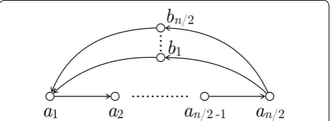
In the next section we discuss how to optimize Algo-rithm 1 to start with a node-covering metagenomic reconstruction of minimum total length. However, there are graphs in which any node-covering metagenomic reconstruction has length �(n2), see Fig. 4.
Additional results
Maximal node‑safe walks without duplicates
In a practical genome assembly setting we want to recon-struct fragments of the genomes as long as possible. As such, we are interested only in maximal node-safe walks, that is, in node-safe walks that are not sub-walks of any other node-safe walk. A trivial way to obtain these is to take the output of Algorithm 1, convert it into the set of all node-safe walks of G, and run a suffix-tree-based algo-rithm for removing the non-maximal ones, in time lin-ear in their total length. However, given a node-covering
circular walk C of length d≤n2, the total length of the
node-safe walks is at most n
k=0kd∈O(n4).
In the next theorem we show how to reduce this time complexity to O(m2+n3logn). The main observation is that a node-safe walk of length k is maximal if it is not extended into a node-safe walk of length k+1. We avoid-ing outputtavoid-ing duplicate maximal walks by traversavoid-ing a suffix-tree built from C to check for previous occurrences of each walk of length k.
Theorem 13 Given a strongly connected graphG withn nodes andm edges, Algorithm 1 can be modified to output the maximal node-safe walks ofG explicitly and without duplicates, with a running time ofO(m2+n3logn).
Proof Let C=(v0,. . .,vd =v0) be a node-covering cir-cular walk C of G, of length n≤d≤n2. At any position in C there can start the occurrence of at most one max-imal node-safe walk. By Corollary 3, the length of each node-safe walk is at most n, thus the sum of the lengths of all maximal node-safe walks of G is O(n3). This implies that if we find the occurrences in C of all maximal node-safe walks without duplicates, then we can output all of them explicitly within the stated time bound.
A node-safe walk w of length k is maximal if no occur-rence C(i, k) of w in C was extended left or right at step
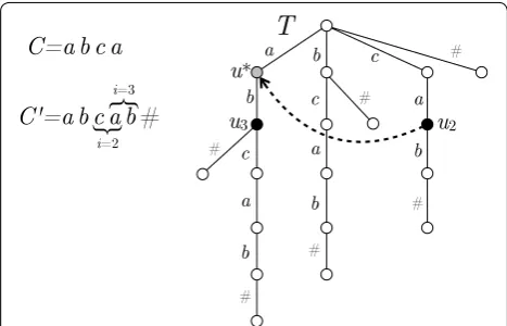
k+1. We can keep track of all previous occurrences of w in C, as follows. Initially, we build the suffix tree T of the (linear) string C′
=v0v1. . .vdv1. . .vn−2# over the alphabet �=V(G)∪ {#}, where # is a new symbol. This
takes time linear in the size of C′
and in the alphabet size || =n, thus O(n2) [47]. As we scan C for a length
k+1∈ {1,. . .,n}, we maintain, as we discuss below, a pointer in T to the node ui such that the label of the path from the root to ui spells C(i, k). In ui we store the infor-mation of whether any occurrence the walk w=C(i,k) was extended at step k+1.
As we advance from i to i+1, we follow a so-called suffix-link in T to move to the node u∗
such that the label from the root of T to u∗
spells C(i+1,k−1) (i.e., C(i, k) with its first character removed). For a detailed discus-sion on the properties of the suffix tree, see e.g., [48]. We then follow the normal tree edge exiting from u∗
labeled vi+1 modd. We thus advance to the node ui+1 of T such that the path from the root to ui+1 spells C(i+1,k). See Fig. 5 for an illustration. After traversing once C at step
k+1 and detecting which node-safe walks of length k are maximal, we traverse C again to output these node-safe walk.
After building the suffix tree using [47], the children of each node are organized in lexicographic order. Descend-ing in the tree takes at most O(log(|�|))=O(logn) time per step for binary searching the first character of Fig. 4 An extremal graph G showing that the upper bound on the
complexity of Algorithm 1 from Theorem 12 is attained. The vertex set of G is {a1,. . .,an/2,b1,. . .,bn/2}. Any node- or edge-covering metagenomic reconstruction of G consists of circular walk(s) whose total length is �(n2
each edge. Following suffix links can be be amortized to the descending operations [48]. Thus, the above addi-tional phase takes time O(n3logn). The pre-compu-tations needed in the proof of Theorem 12 take time O(m2+n3) , from which the claimed time complexity
bound follows.
The algorithm for finding edge‑safe walks
In this section we adapt Algorithm 1 and its implemen-tation to find edge-safe walks, as characterized by The-orem 4. This will result in an algorithm running in time O(m2n). The proof of the following theorem is entirely analogous to the node-safe case.
Theorem 14 LetG be a strongly connected graph withn nodes andm edges. In time we can output an edge-cover-ing circular walk O(m2n)C, and the set of all pairs (i, k) such thatC(i, k) is an edge-safe walk ofG.
Proof The proof is analogous to the node-safe case, and thus we briefly sketch the differences. In the edge-cover-ing case, the set of certificates of a walk w consists of the edges e such that all cycles passing through e contain w as sub-walk. Analogously to Lemma 6, we have that the set of certificates of a walk w equals the intersection of the sets of certificates of its individual edges. The algorithm for the edge-safe case is that same as Algorithm 1, with the difference that we now start with an edge-covering circular walk C and we do not check anymore that each C(i, 1) is the only vi–vi+1 path.
By the same argument given in the proof of Theo-rem 12, such a circular walk C has length at most mn and can be found in time O(mn). The certificates of all edges can be similarly computed in time O(m2) (now there is no need to subdivide nodes into single edges). Lemma 9 can be applied verbatim without modifications. The analog of Lemma 11 now starts with an edge-covering circular walk C of length O(mn). The only difference in its proof is that the sets of certificates now have size at most m, thus their intersection takes time O(m). This implies that we can pre-compute G and C in time O(m2n).
After this pre-processing phase, the algorithm itself works in time O(mn2), since the edge-covering circular
walk C has length O(mn).
With a proof identical to the one of Theorem 13, we also obtain the following result.
Theorem 15 Given a strongly connected graph G with n nodes andm edges, we can output the maximal edge-safe walks ofG explicitly and without duplicates, in time ofO(m2nlogn).
Optimizations to the algorithms
A trivial way to optimize Algorithm 1 is to start with a node-covering circular walk of minimum length. How-ever, this is an NP-hard problem, since G has a node-covering circular walk of length n if and only if G is Hamiltonian. Observe though that instead of a single covering circular walk, we can start with a node-covering metagenomic reconstruction possibly consist-ing of multiple circular walks, and apply Algorithm 1 to each walk in the reconstruction. This is correct by defini-tion, since node-safe walks are sub-walks of some walk in any node-covering metagenomic reconstruction.
Finding a node-covering metagenomic reconstruction whose circular walks have minimum total length can be solved with a minimum-cost circulation problem (see e.g., [49, 50] for basic results on minimum-cost circula-tions). From G, we construct the graph G′
by subdivid-ing every node of G once (recall the construction from Lemma 8). We set demand 1 and cost 0 on each edge (xin,xout), with x∈V(G). On all edges corresponding to
original edges of G we set demand 0 and cost 1. A circu-lation f in G′
satisfying the demands can be decomposed into cycles, which form a node-covering metagen-omic reconstruction in G. The total length of these cycles in G equals the cost of f. Since G′
has no capaci-ties, a minimum-cost circulation in G′
can be found in time O(nlogU(m+nlogn)), where U is the maximum Fig. 5 Illustration of the proof of Theorem 13; we are scanning C with
value of a demand, using the algorithm of Gabow and Tarjan [51]. All demands in G′
are 1, thus this bound becomes O(nm+n2logn).
In the algorithm for finding all edge-covering circular walks, we need to find an edge-reconstruction whose circular walks have minimum total length. This can be solved as above, without subdividing the nodes of G. We add to every edge the demand 1 and cost 1 and then com-pute a minimum-cost circulation. The decomposition of the optimal circulation into cycles forms an edge-recon-struction of G.
Conclusions and future work
We consider [19] and the present work as starting points for characterizing all safe solutions for natural assembly problem formulations, and thus obtaining safe and com-plete algorithms.
As future work, we plan to study formulations where the assembly solution is made up of non-circular cover-ing walks, or where the assembly solutions consist of a given number of covering walks (e.g., a given number of chromosomes). In terms of real graph instances, the worst-case complexity of our algorithm may be prohibi-tive, and thus improving it is an important problem.
We also leave for future work an idealized experimen-tal study similar to what was done for the single genome case in [19]. This compared the lengths and biological content of some classes of safe solutions known in the lit-erature, on de Bruijn graphs constructed from error-free, single-stranded simulated reads.
The ultimate goal of a “safe and complete” approach is to be adapted to the peculiarities of real data, such as sequencing errors, insufficient sequencing coverage, reverse complements. However, our belief is that we first need a clean and solid theoretical foundation, which can later be extended, or weakened, to account for such features.
Authors’ contributions
NOA and AIT devised the problem formulation, NOA found the graph-theoretic characterizations of safe walks, and NOA, VM and AIT devised the algorithms. All authors read and approved the final manuscript.
Acknowledgements
We thank Paul Medvedev for discussions on the proof of Theorem 4, and Martin Milanič for pointing us topersistent solutions and blockers.
Competing interests
The authors declare that they have no competing interests.
Availability of data and materials
Not applicable.
Consent for publication
Not applicable.
Ethics approval and consent to participate
Not applicable.
Funding
This work was partially supported by the Academy of Finland under Grant 284598 (CoECGR) to NOA and VM and Grant 274977 to AIT.
Publisher’s Note
Springer Nature remains neutral with regard to jurisdictional claims in pub-lished maps and institutional affiliations.
Received: 10 February 2017 Accepted: 20 January 2018
References
1. Miller JR, Koren S, Sutton G. Assembly algorithms for next-generation sequencing data. Genomics. 2010;95(6):315–27.
2. Nagarajan N, Pop M. Sequence assembly demystified. Nat Rev Genet. 2013;14(3):157–67.
3. Simpson JT, Pop M. The theory and practice of genome sequence assembly. Annu Rev Genom Hum Genet. 2015;16:153–62. https://doi. org/10.1146/annurev-genom-090314-050032.
4. Myers EW. The fragment assembly string graph. Bioinformatics. 2005;21(suppl–2):79–85.
5. Simpson JT, Durbin R. Efficient de novo assembly of large genomes using compressed data structures. Genome Res. 2011;22(3):549–56.
6. Idury RM, Waterman MS. A new algorithm for DNA sequence assembly. J Comput Biol. 1995;2(2):291–306.
7. Pevzner PA, Tang H, Waterman MS. An Eulerian path approach to DNA fragment assembly. Proc Nat Acad Sci. 2001;98:9748–53.
8. Nagarajan N, Pop M. Parametric complexity of sequence assembly: theory and applications to next generation sequencing. J Comput Biol. 2009;16(7):897–908.
9. Medvedev P, Brudno M. Maximum likelihood genome assembly. J Com-put Biol. 2009;16(8):1101–16.
10. Medvedev P, Georgiou K, Myers G, Brudno M. Computability of models for sequence assembly. WABI. 2007;4645:289–301.
11. Kapun E, Tsarev F. De Bruijn superwalk with multiplicities problem is NP-hard. BMC Bioinform. 2013;14(Suppl 5):7.
12. Lysov IP, Florent’ev VL, Khorlin AA, Khrapko KR, Shik VV. Determination of the nucleotide sequence of DNA using hybridization with oligonucleo-tides. A new method. Doklady Akademii nauk SSSR. 1988;303(6):1508–11. 13. Narzisi G, Mishra B, Schatz MC. On algorithmic complexity of
biomolecu-lar sequence assembly problem. Algorithms for computational biology. 2014. Springer, Cham, p. 183–95.
14. Simpson JT, Wong K, Jackman SD, Schein JE, Jones SJ, Birol İ. ABySS: a parallel assembler for short read sequence data. Genome Res. 2009;19(6):1117–23.
15. Butler J, Maccallum I, Kleber M, Shlyakhter IA, Belmonte MK, Lander ES, Nusbaum C, Jaffe DB. Allpaths: de novo assembly of whole-genome shotgun microreads. Genome Res. 2008;18(5):810–20.
16. Li R, Zhu H, Ruan J, Qian W, Fang X, Shi Z, Li Y, Li S, Shan G, Kristiansen K. De novo assembly of human genomes with massively parallel short read sequencing. Genome Res. 2010;20(2):265.
17. Iqbal Z, Caccamo M, Turner I, Flicek P, McVean G. De novo assembly and genotyping of variants using colored de Bruijn graphs. Nat Genet. 2012;44(2):226–32.
18. Zerbino DR, Birney E. Velvet: algorithms for de novo short read assembly using de Bruijn graphs. Genome Res. 2008;18(5):821–9.
19. Tomescu AI, Medvedev P. Safe and complete contig assembly via omnit-igs. In: Singh M. (ed.). Research in computational molecular biology-20th annual conference, RECOMB 2016, Santa Monica, CA, USA, April 17–21, 2016. In: Proceedings lecture notes in computer science. 2016, vol 9649, p. 152– 63. Springer, cham. https://doi.org/10.1007/978-3-319-31957-5. 20. Kececioglu JD, Myers EW. Combinatiorial algorithms for DNA sequence
assembly. Algorithmica. 1995;13(1/2):7–51.
21. Jackson BG. Parallel methods for short read assembly. Ph.D. Thesis, Iowa State University. 2009.
• We accept pre-submission inquiries
• Our selector tool helps you to find the most relevant journal • We provide round the clock customer support
• Convenient online submission • Thorough peer review
• Inclusion in PubMed and all major indexing services • Maximum visibility for your research
Submit your manuscript at www.biomedcentral.com/submit
Submit your next manuscript to BioMed Central
and we will help you at every step:
23. Venter JC, Remington K, Heidelberg JF, Halpern AL, Rusch D, Eisen JA, Wu D, Paulsen I, Nelson KE, Nelson W, Fouts DE, Levy S, Knap AH, Lomas MW, Nealson K, White O, Peterson J, Hoffman J, Parsons R, Baden-Tillson H, Pfannkoch C, Rogers Y-H, Smith HO. Environmental genome shotgun sequencing of the Sargasso sea. Science. 2004;304(5667):66–77. https:// doi.org/10.1126/science.1093857.
24. Tyson GW, Chapman J, Hugenholtz P, Allen EE, Ram RJ, Richardson PM, Solovyev VV, Rubin EM, Rokhsar DS, Banfield JF. Community structure and metabolism through reconstruction of microbial genomes from the environment. Nature. 2004;428(6978):37–43.
25. Qin J, Li R, Raes J, Arumugam M, Burgdorf KS, Manichanh C, Nielsen T, Pons N, Levenez F, Yamada T, Mende DR, Li J, Xu J, Li S, Li D, Cao J, Wang B, Liang H, Zheng H, Xie Y, Tap J, Lepage P, Bertalan M, Batto J-M, Hansen T, Le Paslier D, Linneberg A, Nielsen HB, Pelletier E, Renault P, Sicheritz-Ponten T, Turner K, Zhu H, Yu C, Li S, Jian M, Zhou Y, Li Y, Zhang X, Li S, Qin N, Yang H, Wang J, Brunak S, Dore J, Guarner F, Kristiansen K, Pedersen O, Parkhill J, Weissenbach J, Bork P, Ehrlich SD, Wang J. A human gut micro-bial gene catalogue established by metagenomic sequencing. Nature. 2010;464(7285):59–65.
26. Veiga P, Gallini CA, Beal C, Michaud M, Delaney ML, DuBois A, Khleb-nikov A, van Hylckama Vlieg JET, Punit S, Glickman JN, Onderdonk A, Glimcher LH, Garrett WS. Bifidobacterium animalis subsp. lactis fermented milk product reduces inflammation by altering a niche for colito-genic microbes. Proc Nat Acad Sci. 2010;107(42):18132–7. https://doi. org/10.1073/pnas.1011737107.
27. Turnbaugh PJ, Hamady M, Yatsunenko T, Cantarel BL, Duncan A, Ley RE, Sogin ML, Jones WJ, Roe BA, Affourtit JP, Egholm M, Henrissat B, Heath AC, Knight R, Gordon JI. A core gut microbiome in obese and lean twins. Nature. 2009;457(7728):480–4. https://doi.org/10.1038/nature07540. 28. Namiki T, Hachiya T, Tanaka H, Sakakibara Y. Metavelvet: an
exten-sion of velvet assembler to de novo metagenome assembly from short sequence reads. Nucleic Acids Res. 2012;40(20):155. https://doi. org/10.1093/nar/gks678.
29. Laserson J, Jojic V, Koller D. Genovo: de novo assembly for metage-nomes. J Comput Biol. 2011;18(3):429–33. https://doi.org/10.1089/ cmb.2010.0244.
30. Peng Y, Leung HCM, Yiu SM, Chin FYL. Meta-idba: a de novo assembler for metagenomic data. Bioinformatics. 2011;27(13):94–101. https://doi. org/10.1093/bioinformatics/btr216.
31. Koren S, Treangen TJ, Pop M. Bambus 2: scaffolding metagenomes. Bioin-formatics. 2011;27(21):2964–71. https://doi.org/10.1093/bioinformatics/ btr520.
32. Peng Y, Leung HCM, Yiu SM, Chin FYL. Idba-ud: a de novo assembler for single-cell and metagenomic sequencing data with highly uneven depth. Bioinformatics. 2012;28(11):1420–8. https://doi.org/10.1093/ bioinformatics/bts174.
33. Boisvert S, Raymond F, Godzaridis É, Laviolette F, Corbeil J, et al. Ray Meta: scalable de novo metagenome assembly and profiling. Genome Biol. 2012;13(12):122.
34. Haider B, Ahn TH, Bushnell B, Chai J, Copeland A, Pan C. Omega: an overlap-graph de novo assembler for metagenomics. Bioinformatics. 2014;30(19):2717–22. https://doi.org/10.1093/bioinformatics/btu395. 35. Vingron M. Near-optimal sequence alignment. Curr Opin Struct Biol.
1996;6(3):346–52.
36. Eppstein D. k-best enumeration. Encyclopedia of algorithms. Berlin: Springer; 2015.
37. Vingron M, Argos P. Determination of reliable regions in protein sequence alignments. Protein Eng. 1990;3(7):565–9. https://doi.org/10.1093/ protein/3.7.565.
38. Chao K-M, et al. Locating well-conserved regions within a pairwise align-ment. Comput Appl Biosci. 1993;9(4):387–96.
39. Costa MC. Persistency in maximum cardinality bipar-tite matchings. Oper Res Lett. 1994;15(3):143–9. https://doi. org/10.1016/0167-6377(94)90049-3.
40. Cechlárová K. Persistency in the assignment and transportation problems. Math Methods Oper Res. 1998;47(2):243–54. https://doi. org/10.1007/BF01194399.
41. Boros E, Golumbic MC, Levit VE. On the number of vertices belonging to all maximum stable sets of a graph. Discret Appl Math. 2002;124(1—-3):17–25. https://doi.org/10.1016/S0166-218X(01)00327-4.
42. Lacko V. Persistency in the traveling salesman problem on halin graphs. Discussiones Mathematicae Graph Theory. 2000;20(2):231–42. https://doi. org/10.7151/dmgt.1122.
43. Zenklusen R, Ries B, Picouleau C, de Werra D, Costa M, Bentz C. Block-ers and transvBlock-ersals. Discret Math. 2009;309(13):4306–14. https://doi. org/10.1016/j.disc.2009.01.006.
44. Costa M, de Werra D, Picouleau C. Minimum d-blockers and d-transversals in graphs. J Comb Optim. 2011;22(4):857–62. https://doi.org/10.1007/ s10878-010-9334-6.
45. Pajouh FM, Boginski V, Pasiliao EL. Minimum vertex blocker clique prob-lem. Networks. 2014;64(1):48–64. https://doi.org/10.1002/net.21556. 46. Italiano GF, Laura L, Santaroni F. Finding strong bridges and strong
articu-lation points in linear time. Theor Comput. 2012;447:74–84. https://doi. org/10.1016/j.tcs.2011.11.011.
47. Farach M. Optimal suffix tree construction with large alphabets. In: Proc. 38th IEEE symposium on foundations of computer science (FOCS). 1997. p. 137–43.
48. Crochemore M, Rytter W. Jewels of stringology. Singapore: World Scien-tific Publishing; 2002. p. 1310.
49. Schrijver A. Combinatorial optimization. Berlin: Springer; 2003.
50. Mäkinen V, Belazzougui D, Cunial F, Tomescu AI. Genome-scale algorithm design. Cambridge: Cambridge University Press; 2015.