RESEARCH
A polynomial time algorithm
for computing the area under a GDT curve
Aleksandar Poleksic
*Abstract
Background: Progress in the field of protein three-dimensional structure prediction depends on the development of new and improved algorithms for measuring the quality of protein models. Perhaps the best descriptor of the quality of a protein model is the GDT function that maps each distance cutoff θ to the number of atoms in the protein model that can be fit under the distance θ from the corresponding atoms in the experimentally determined structure. It has long been known that the area under the graph of this function (GDT_A) can serve as a reliable, single numerical measure of the model quality. Unfortunately, while the well-known GDT_TS metric provides a crude approximation of GDT_A, no algorithm currently exists that is capable of computing accurate estimates of GDT_A.
Methods: We prove that GDT_A is well defined and that it can be approximated by the Riemann sums, using avail-able methods for computing accurate (near-optimal) GDT function values.
Results: In contrast to the GDT_TS metric, GDT_A is neither insensitive to large nor oversensitive to small changes in model’s coordinates. Moreover, the problem of computing GDT_A is tractable. More specifically, GDT_A can be com-puted in cubic asymptotic time in the size of the protein model.
Conclusions: This paper presents the first algorithm capable of computing the near-optimal estimates of the area under the GDT function for a protein model. We believe that the techniques implemented in our algorithm will pave ways for the development of more practical and reliable procedures for estimating 3D model quality.
Keywords: Protein structure, Structure modeling, Structure prediction, Model quality
© 2015 Poleksic. This article is distributed under the terms of the Creative Commons Attribution 4.0 International License (http:// creativecommons.org/licenses/by/4.0/), which permits unrestricted use, distribution, and reproduction in any medium, provided you give appropriate credit to the original author(s) and the source, provide a link to the Creative Commons license, and indicate if changes were made. The Creative Commons Public Domain Dedication waiver (http://creativecommons.org/publicdomain/ zero/1.0/) applies to the data made available in this article, unless otherwise stated.
Background
Advances in the area of protein three-dimensional structure prediction depend on the ability to accurately measure the quality of a protein model. One of the most popular and most reliable measure of the protein model quality is GDT_TS. It is defined as the average value of
GDT_Pθ computed for four distance cutoffs θ =2i,
i=0, 3, where GDT_Pθ is the percentage of model
resi-dues (represented by their Cα atoms) that can be placed
under θ ångströms from the corresponding residues in the experimental structure [1, 2]. In a “high-accuracy” version of GDT_TS, denoted by GDT_HA, the distance cutoffs are cut in half (θ =2i, i= −1, 2) [3]. In both
approaches, the underlying assumption is that the experi-mental (crystallographic or NMR) structure is close to
the real (native) structure (which is sometimes not true due to experimental errors).
Several methods exist for computing GDT_TS. The LGA algorithm [4] can estimate GDT_TS quickly, but those estimates deviate from the true GDT_TS values in about 10 % of the cases [5]. Rigorous algorithms for com-puting GDT_TS have also been developed [6–9], but they are computationally much more expensive.
The GDT_TS is commonly interpreted as an approxi-mation of the area under the GDT curve, denoted by
GDT_A [10–12]. Unfortunately, since the measure is approximated using the GDT function values at only sev-eral distance cutoffs, the errors in the area approxima-tion are large. As we demonstrate later, GDT_TS is not only overly sensitive to small but also insensitive to large changes in the protein model’s coordinates.
In this paper, we present a polynomial time algorithm for computing GDT_A. Our method runs on the order
Open Access
*Correspondence: [email protected]
O(n3), where n represents the length of the protein model
(and O hides the log factor). The algorithm returns
“near-optimal” GDT_A scores, meaning that the errors in our estimates can be made arbitrary small i.e., smaller than any upfront specified vale. Although our method is theo-retical, we believe that its parallel implementations, cou-pled with carefully designed speed up techniques, can result in a practical and widely used software tool.
The rest of this paper is structured as follows. First, we present three examples that illustrate drawbacks of
GDT_TS and advantages of GDT_A. Then, we place our theory on a firm mathematical ground, which enables us to formally define the GDT_A computation problem. Finally, we describe the actual algorithm for GDT_A and provide its running time analysis.
Methods
Definition of the GDT function
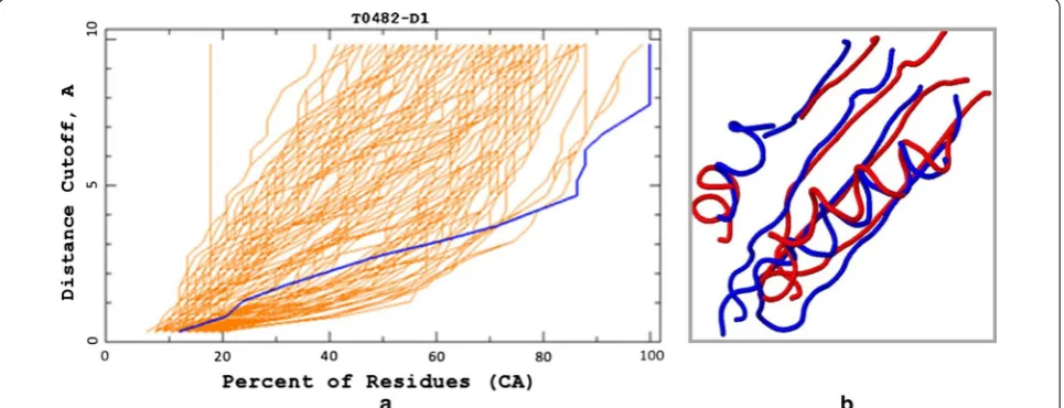
The GDT function is a mapping that relates each distance cutoff θ to the percentage of model residues that can be placed at distance ≤θ from the corresponding residues in the experimentally determined structure. The graph of a
GDT function provides a valuable insight into the quality of a protein model (Fig. 1). More specifically, the closer the graph runs to the horizontal axis (in other words, the smaller the area under the graph), the better the model.
As a single numerical measure of the model quality,
GDT_TS is extensively used at CASP to rank different models for the same target [13, 14]. Since it represents the average of GDT_Pθ at several distance cutoffs, GDT_TS is
often viewed as an approximation of the area under the
GDT curve (GDT_A) [10–12]:
However, as we demonstrate below, such a sparse sam-pling of the values of GDT function compromises the reliability of GDT_TS.
In our first example, we analyze the protein model for the target T0482, submitted by the group TS208 at CASP8 (Fig. 1). The GDT_TS score of this particular model was not even among the best dozen at CASP8, despite the fact that it fits the largest number of residues at distance ≤∼4 from the corresponding residues in the
experimental structure. In fact, the blue model (Fig. 1a) can be superimposed onto the experimental structure so that all of its residues are at distance ≤8 from the
resi-dues in the experimental structure (Fig. 1b), while no such superposition exists for any other model, even for the distance cutoff of 10Å. Interestingly, according to the MAMMOTH algorithm [15], the blue model is the best model for this particular target, while the DALI [16] algo-rithm ranks it as the second best.
Although it is impossible to tell whether #13 GDT_TS
rank is more or less fair than #1 and #2 rank assigned by MAMMOTH and DALI, respectively, it is also not difficult to see that the ranking by the area under the
GDT plot (GDT_A) would serve as a good compromise between these extremes.
The next two examples illustrate further disadvantages of GDT_TS. As seen in Fig. 2, better GDT_TS scores can be assigned to obviously worse models. Moreover, as demonstrated in Fig. 3, very similar models can have sig-nificantly different GDT_TS scores.
(1)
GDT_TS=
3
i=0
GDT_P2i.
Mathematical formalism
Strictly speaking, the GDT function is not well-defined. Zooming into the plot of the model highlighted in Fig. 1a, we see a set of many small vertical segments, meaning that each point on the horizontal axis is mapped to zero or more points on the vertical axis (Fig. 4). On the other hand, the inverse function (mapping each distance cut-offs θ to the percentage of residues in the model structure that can be fit under the distance θ from the correspond-ing residues in the experimental structure) is obviously well defined. This allows us to define the area under the GDT plot as the complement of the area under the inverse function:
where Total_Area represents the area of the rectan-gular region under consideration (100 × 10). We start
our mathematical formalism by first defining a protein structure.
(2) GDT_A=Total_Area−GDT_A
Definition 1 A protein structure a is a sequence of points in the three dimensional Euclidean space R3
The sequence elements ai can represent individual atoms, but it is more typical (in particular in protein structure prediction experiments) to assume that each point ai corresponds to the alpha-carbon atom of the protein’s ith amino acid.
In what follows, we formally define the GDT function [17]. For simplicity of presentation, we will modify the codomain of GDT to represent the “fraction of residues” (ranging from 0 to 1) instead of “percentages of residues” (ranging from 0 to 100). We note that this simple res-caling of the ordinate values will have no effects on the results obtained in our study.
Definition 2 Let a=(a1,. . .,an) be a
pro-tein structure consisting of n amino acids, let
b=(b1,. . .,bn) be a 3D model of a, and let θ be a
posi-tive constant. The Hubbard function (or GDT
func-tion) is the function Hb: [0,θ] →(0, 1], defined by Hb(θ )=maxτ|{i| �ai−τ (bi)� ≤θ}|/n, where
denotes the Euclidean norm on R3 and τ is a rigid
trans-formation (a composition of a rotation and a translation).
Theorem 1 Hb is a stepwise function with finitely many stepsθ1,. . .,θk, 1 ≤ k ≤ n − 1.
Proof Since Hb is monotony non-decreasing and since the
range of Hb is a finite subset of (0,1], it follows that Hb must
be a stepwise function. To complete the proof, we note that the number of steps in Hb matches the size of its range,
which does not exceed n − 1, where n is the length of b.
For simplicity of presentation, from now on (and when-ever the model b is implied), we will omit the subscript in
Hb and denote the Hubbard function only by H.
(3) a=(a1,. . .,an).
Fig. 2 Insensitivity of GDT_TS. This theoretical example shows no sensitivity of GDT_TS to large variations in model quality. Surprisingly, the red model has a better GDT_TS score than the better blue model, even though it is worse by all standards. Notice that, unlike GDT_TS, the GDT_A measure is not skewed by the values at the cutoff points 1, 2, 4 and 8 Å. In fact, the GDT_A score of the blue model is twice as good as that of the red model
Algorithm for GDT_A
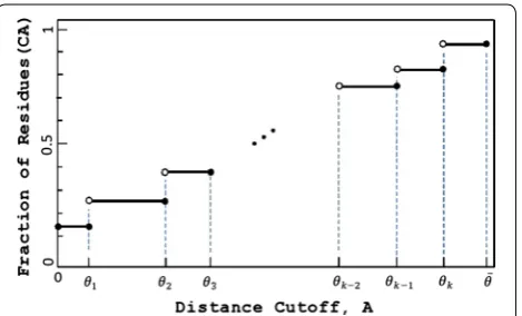
The area under H is the sum of the areas of the rectangu-lar regions (θi)(θi − θi−1):
where θ0 = 0 and θk+1=θ (Fig. 5). It would be trivial to compute Area had we known all θi and all function
val-ues H(θi). Unfortunately, even if we knew the step points θi, it would be computationally very difficult to compute
the function values at them, since the best to date algo-rithm for computing H(θi) runs on the order of O(n7) [7].
Hence, we resort to using the Riemann sums to approxi-mate (instead of to compute exactly) the area under the graph of H.
The following definition and an accompanying theo-rem can be found in virtually any mathematical analysis textbook.
Definition 3 If f :[a,b]→R is a function then
R=
n
i=1
vi(xi−xi−1), where a = x0 < x1 < ··· < xn = b
is the partition of the interval [a, b] and vi denotes the
supremum of f over [xi−1, xi], is called the upper Riemann sum of f on [a, b].
Theorem 2 Let f be a real, non-decreasing, Riemann integrable function on an interval [a, b]. Then
(4) Area=
k+1
i=1
H(θi)(θi−θi−1),
(5)
b
a
f(x)dx−R
< �x
f(b)−f(a),
where
is the upper Riemann sum of f the and x= maxi(xi−xi−1).
Observe that, since Hb is piecewise continuous, it must
be integrable on [0,θ]. Thus, the area under the graph of H is
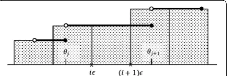
To approximate Area with a Riemann sum, one can
define the partition points ǫ, 2ǫ,. . .,mǫ, where m= ⌈θ /ǫ⌉
(Fig. 6) and then compute an estimate Area(ǫ ) of Area as (6) R=
n
i=1
vi(xi−xi−1)
(7) Area=
θ
0
H(θ )dθ.
Fig. 4 A closer look at the GDT_TS function. Zooming into the GDT plot of the model highlighted in Fig. 1. What appears to be the graph of a con-tinuous function is, in fact, a set consisting of many separated vertical line segments
Fig. 5 The general shape of the Hubbard function. Notice that the values θi along with the function values Hb(θi), i=1,k, uniquely determine the area under the graph of Hb. At the biannual CASP
The error |Area – Area (ǫ)| in the estimate (8) is below 2ǫ.
Up to a half of this error is due to the error in the Rie-mann sum with the remaining error being due to the pos-sible placement of the last partition point mǫ outside the
interval [0,θ].
Unfortunately, computing the area estimates accord-ing to (8) is still a challenging problem, because (as we mentioned above), there is no computationally effective procedure for finding the function values H(iǫ). To
cir-cumvent the problem, we utilize an efficient algorithm capable of computing the lower bound estimates Hi of H(iǫ), satisfying H((i−1)ǫ)≤Hi≤H(iǫ), i=1,m. We then compute an estimate Area(ǫ) of Area as
Since Area(ǫ)−Area(ǫ)
<2ǫ, it follows that
Area(ǫ) is a 4ǫ-approximation of Area. Below we show
how to compute all Hi’s, and, in turn, Area(ǫ) in time
On3logn/ǫ6, where n is the length of b. Our algorithm
takes advantage of an efficient procedure for computing near optimal GDT_TS values [5].
Let T(b) denotes the image of the model structure
b under the transformation T. Denote by MAX(T,θ )
the largest fraction of residues from T(b) that are at distance ≤θ from the corresponding residues in the experimental structure a. To find each Hi, it is enough
to compute a rigid body transformation Ti satisfying H((i−1)ǫ)≤MAX(Ti,iǫ)≤H(iǫ).
Denote by Tθ a transformation that places a
larg-est subset bθ of residues from b at distance ≤θ from the
corresponding residues in the experimental structure. Given Tθ, one can easily compute bθ by calculating all n
distances between the residues ai and Tθ(bi). Note that (8) Area(ǫ)=
m
i=1 ǫH(iǫ)
(9)
Area(ǫ)= m
i=1 ǫHi.
P(Tθ, θ) = H(θ). We approximate the transformation Tθ
by a so-called “near-optimal” transformation i.e., a trans-formation that places at least as many residues from the model structure under distance θ+ǫ as the optimal
transformation Tθ places under the distance θ. From now
on, we will use Tǫ
θ to denote a “near-optimal”
transforma-tion and the corresponding set of residues will be denoted by bǫ
θ. Observe that P
Tǫ θ,θ+ǫ
≥P(Tθ,θ )=H(θ ). Building upon any procedure for computing Tǫ
θ, one
can develop an algorithm for Area(ǫ) by substituting PTǫ
θi,θi+ǫ
for Hi in (10), where θi=(i−1)ǫ. Several
existing methods can be modified and made suitable for finding Tǫ
θ. The most efficient such method relies on the
concept of “radial pair” [5].
Definition 4 Let S= {s1,. . .,sn} be a set of points in the three-dimensional Euclidean space. An ordered pair of points (si,sj) is called a radial pair of S if sj is the
fur-thest point from si among all points in S.
Theorem 3 Let T1 andT2 be two transformations and let(sk,sl) be a radial pair of S. If �T1(sk)−T2(sk)�< ǫ/3 and�T1(sl)−T2(sl)�< ǫ/3 then there exists a rota-tion Raround the line through T1(sk) andT1(sl)such that �RT1sp
−T2(sp)�< ǫ, for any sp inS. The rotation R can be found in time O (nlogn), where n is the size of S.
A proof of the above theorem can be found in [5]. The algorithm for finding R is fairly straightforward and it relies on the so-called plane-sweep approach [18].
The Theorem 3 implies that one choice for the near-optimal transformation Tθǫ is the transformation R ∘ T,
where T is any transformation that maps the points bk
and bl from the radial pair (bk, bl) of bθ to the ǫ/3
neigh-borhoods of Tθ(bk) and Tθ(bl), respectively, and R is the
rotation around the radial axis T(bk)T(bl) that maps the remaining points from T(bθ) to the ǫ-neighborhoods of
the corresponding points from Tθ(bθ).
In search for a radial pair of bθ, the algorithm in [5]
explores all n2 possible pairs of residues in b. For each
candidate radial pair (bk,bl), the algorithm
gener-ates a finite, representative set of transformations that map bk and bl into θ+ǫ/3 neighborhoods of ak and al,
respectively (see the paragraph below for more details). For every such transformation T, a plane-sweep algo-rithm [18] is used to find a rotation R around the axis
T(bk)T(bl) that maximizes the number of residues from
R(T(b)) that can be placed at distance < θ+ǫ from the corresponding residues in a.
A finite set of transformations that map the resi-dues bk and bl into the θ+ǫ/3 neighborhoods of ak
and al, respectively, is constructed in such a way to
ensure that for at least one of those transformation T,
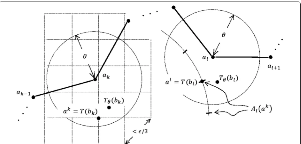
�T(bk)−Tθ(bk)�< ǫ/3 and �T(bl)−Tθ(bl)�< ǫ/3. This can be achieved by partitioning R3 into small cubes
of side length slightly smaller than √3ǫ/9 and then
col-lecting the vertices of the cubes that are inside the open ball of radius θ+ǫ/6 around ak (Fig. 7). The elements of this set, denoted by Ak, are the candidate points T(bk).
The number of points in Ak is O(1/ǫ3) and at least one
of them must be at distance < ǫ/6 from Tθ(bk) (Fig. 7). For each point ak ∊ A
k, the set Al(ak) of possible images of bl under T is computed by discretizing the spherical cap
S(ak,�b
k−bl�)∩B(al,θ+ǫ/3), where S(a, r) and B(a, r)
denote the sphere and the open ball in R3 with center a
and radius r, respectively, in such a way that at least one point from Al(ak) is found at distance < ǫ/3 from Tθ(bl)
(Fig. 7). We note that size of Al(ak) is O(1/ǫ2). Hence, the
total number of candidate pairs of points (T(bk), T(bl)) is O(1/ǫ5).
An obvious to compute Tǫ
θ1,. . .,T
ǫ
θm is to run the
just described algorithm m times in succession, for
θ =θ1,. . .,θ =θm. However, such an approach results
in many unnecessary repeated calculations as the area around ak and the corresponding spherical cap in the
neighborhoods of al are discretized over and over again.
Moreover, all transformations T and R, generated and inspected during the procedure for finding Tǫ
θi, are inspected again during the procedure for finding Tǫ
θj, for each j > i.
Fig. 7 Discretizing the space of rigid body transformations. 2D illustration of Ak (the set of the vertices of the squares shown on the left) and the set
We show that all transformations Tθǫ1,. . .,Tθǫm and the corresponding values H1, …, Hm can be computed, at once, during the procedure of finding the last transfor-mation, namely Tθmǫ. As demonstrated in the pseudocode above, the transformation T is generated only once for each pair of points ak,al∈Ak×Al
ak and a sweep-plane algorithm for finding R is called only once for each i
satisfying �ak−ak�< θi+ǫ/6 and �al−al�< θi+ǫ/3.
The values of Hi are updated on the fly.
Running time analysis
To analyze the algorithm’s running time, we note that the number of iterations of the first for loop is equal to the number of candidate radial pairs (bk, bl), which is
On2. The number of iterations of the second for loop matches the number of pairs of grid points around ak and al, which is O1/ǫ3
×O1/ǫ2=O1/ǫ5. Each one of O(m)=O(⌈ ¯θ /ǫ⌉)=O(1/ǫ) iterations of the third for
loop calls a O(nlogn) plane-sweep procedure to compute
an optimal rotation and (if needed) to update the value
Hi. Hence, the asymptotic time complexity of the three nested for loops is On3logn/ǫ6.
Conclusions
Estimating the quality of a protein 3D model is a chal-lenging task. Automatically generated GDT_TS score is helpful as the first raw approximation but this measure is neither sensitive nor selective enough to be exclusively relied upon in ranking different models for the same tar-get. In this paper, we show that using a more accurate approximation of the area under the GDT curve as the criterion of model quality addresses many of the draw-backs of GDT_TS. We also present a rigorous On3
Despite the cubic asymptotic running time with a relatively large hidden constant, we believe that the techniques presented in this paper can guide a future development of a computationally efficient computer program, in particular since our methodology is amena-ble to parallel implementations. A heuristic version of the algorithm for estimating the area under the GDT plot can be found at http://bioinfo.cs.uni.edu/GDT_A.html.
Acknowledgements
This project was supported by the University of Northern Iowa Professional Development Award. The structure alignment figures were prepared in Jmol (http://www.jmol.org).
Competing interests
The author declares that there is no competing interests regarding the publi-cation of this article.
Received: 7 March 2015 Accepted: 9 October 2015
References
1. Zemla A, Venclovas C, Moult J, Fidelis K. Processing and analysis of CASP3 protein structure predictions. Proteins. 1999;37(S3):22–9.
2. Zemla A, Venclovas C, Moult J, Fidelis K. Processing and evaluation of predictions in CASP4. Proteins. 2001;45(S5):13–21.
3. Read RJ, Chavali G. Assessment of CASP7 predictions in the high accuracy template-based modeling category. Proteins. 2007;69(S8):27–37. 4. Zemla A. LGA—a method for finding 3D similarities in protein structures.
Nucleic Acids Res. 2003;31:3370–4.
5. Li SC, Bu D, Xu J, Li M. Finding nearly optimal GDT scores. J Comput Biol. 2011;18(5):693–704.
6. Li SC, Ng YK. On protein structure alignment under distance constraint. Theor Comput Sci. 2011;412:4187–99.
7. Choi V, Goyal N. A combinatorial shape matching algorithm for rigid protein docking. CPM Lecture Notes Comput Sci. 2004;3109:285–96. 8. Akutsu T. Protein structure alignment using dynamic programming and
iterative improvement. IEICE Trans Ins Syst. 1995; E79-D(12):1629–36. 9. Poleksic A. Improved algorithms for matching r-separated sets with
applications to protein structure alignment. IEEE/ACM Trans Comput Biol Bioinform. 2013;10(1):226–9.
10. Kryshtafovych A, Fidelis K, Moult J. CASP8 results in context of previous experiments. Proteins. 2009;77(9):217–28.
11. Tramontano A, Cozzetto D, Giorgetti A, Raimondo D. The assess-ment of methods for protein structure prediction. Methods Mol Biol. 2008;413:43–57.
12. Kryshtafovych A, Milostan M, Szajkowski L, Daniluk P, Fidelis K. CASP6 data processing and automatic evaluation at the protein structure prediction center. Proteins. 2005;61(S7):19–23.
13. Huang YJ, Mao B, Aramini JM, Montelione GT. Assessment of template-based protein structure predictions in CASP10. Proteins. 2014;82(S2):43–56.
14. Tai CH, Bai H, Taylor TJ, Lee B. Assessment of template-free modeling in CASP10 and ROLL. Proteins. 2014;82(S2):57–83.
15. Ortiz AR, Strauss CE, Olmea O. MAMMOTH (matching molecular models obtained from theory): an automated method for model comparison. Protein Sci. 2002;11:2606–21.
16. Holm L, Sander C. Protein structure comparison by alignment of distance matrices. J Mol Biol. 1993;233:123–38.
17. Pevsner J. Bioinformatics and functional genomics. 2nd edn. Wiley-Black-well; 2009.
18. Alt H, Mehlhorn K, Wagener H, Welzl E. Congruence, similarity, and sym-metries of geometric objects. Dicrete Comput Geom. 1988;3:237–56.
Submit your next manuscript to BioMed Central and take full advantage of:
• Convenient online submission • Thorough peer review
• No space constraints or color figure charges • Immediate publication on acceptance
• Inclusion in PubMed, CAS, Scopus and Google Scholar • Research which is freely available for redistribution