R E S E A R C H
Open Access
An online peak extraction algorithm for ion
mobility spectrometry data
Dominik Kopczynski
1and Sven Rahmann
1,2*Abstract
Ion mobility (IM) spectrometry (IMS), coupled with multi-capillary columns (MCCs), has been gaining importance for biotechnological and medical applications because of its ability to detect and quantify volatile organic compounds (VOC) at low concentrations in the air or in exhaled breath at ambient pressure and temperature. Ongoing
miniaturization of spectrometers creates the need for reliable data analysis on-the-fly in small embedded low-power devices. We present the first fully automated online peak extraction method for MCC/IMS measurements consisting of several thousand individual spectra. Each individual spectrum is processed as it arrives, removing the need to store the measurement before starting the analysis, as is currently the state of the art. Thus the analysis device can be an inexpensive low-power system such as the Raspberry Pi.
The key idea is to extract one-dimensional peak models (with four parameters) from each spectrum and then merge these into peak chains and finally two-dimensional peak models. We describe the different algorithmic steps in detail and evaluate the online method against state-of-the-art peak extraction methods.
Keywords: Ion mobility spectrometry, Peak detection, Automated data analysis, Online analysis
Introduction
Ion mobility (IM) spectrometry (IMS), coupled with multi-capillary columns (MCCs), MCC/IMS for short, has been gaining importance for biotechnological and medical applications. With MCC/IMS, one can measure the pres-ence and concentration of volatile organic compounds (VOCs) in the air or in exhaled breath with high sensitiv-ity. In contrast to other technologies, such as mass spec-trometry coupled with gas chromatography (GC/MS), MCC/IMS works at ambient pressure and temperature. Several diseases like chronic obstructive pulmonary dis-ease (COPD) [1], sarcoidosis [2] or lung cancer [3] can potentially be diagnosed early with MCC/IMS technology. IMS is also used for the detection of drugs [4] and explo-sives [5]. Constant monitoring of VOC levels is of inter-est in biotechnology, e.g., for watching fermenters with yeast producing desired compounds [6] and in medicine, e.g., monitoring propofol levels in the exhaled breath of patients during surgery [7].
*Correspondence: [email protected]
1Bioinformatics for High-Throughput Technologies, Computer Science XI, and Collaborative Research Center SFB 876, TU Dortmund, Dortmund, Germany 2Genome Informatics, Institute of Human Genetics, University Hospital Essen, University of Duisburg-Essen, Essen, Germany
IMS technology is moving towards miniaturization and small mobile devices. This creates new challenges for data analysis: The analysis should be possiblewithinthe measuring device without requiring additional hardware like an external laptop or a compute server. Ideally, the spectra can be processed on a small embedded chip or small device like a Raspberry Pi or similar hardware with restricted resources. Algorithms in small mobile hard-ware face constraints, such as the need to use little energy (hence little random access memory), while maintaining prescribed time constraints.
The basis of MCC/IMS analysis ispeak extraction, by which we mean a representation of all high-intensity regions (peaks) in the measurement by using a few descriptive parameters per peak instead of the full mea-surement data. State-of-the-art software (like IPHEx [8], Visual Now [9], PEAX [10]) only extracts peaks when the whole measurement is available, which may take up to 10 minutes because of the pre-separation of the ana-lytes in the MCC. Our own PEAX software in fact defines modular pipelines for fully automatic peak extraction and compares favorably with a human domain expert doing the same work manually when presented with a whole MCC/IMS measurement. However, storing the whole
measurement is not desirable or possible when the mem-ory and CPU power is restricted. Here we introduce a method to extract peaks and estimate a parametric repre-sentation while the measurement is being captured. This is called online peak extraction, and this article presents the first algorithm for this purpose on MCC/IMS data. An extended abstract of this work has been published at WABI’14 [11].
Section ‘Background’ introduces the necessary back-ground on the data produced by an MCC/IMS experi-ment, on peak modeling and on optimization methods. The basic idea of our algorithm is to process each IM spec-trum as soon as it arrives (and before the next one arrives). After appropriate pre-processing including denoising and baseline correction described in Section ‘Denoising and baseline correction’, the single spectra are reduced into a mixture of parametric one-dimensional peak models, described in Section ‘Reducing a spectrum to peak mod-els’. Accordingly, in Section ‘Aligning consecutive spec-trum peak lists’ the approach of connecting models from two subsequent spectra into peak chains is explained. The main challenge is then to merge the peak chains into two-dimensional peak models, described in Section ‘Estimating 2-D peak models’. In Section ‘Peak clustering’ we introduce a novel approach for clustering peaks among several measurements e.g. for time series. An evalua-tion of our approach is presented in Secevalua-tion ‘Evaluaevalua-tion’ including a listing of all settings of the MCC/IMS as well as an explanation of all adjustable parameters, while Section ‘Discussion and conclusion’ contains a concluding discussion.
Background
Ion mobility spectrometers and their functions are well documented [12], and we do not go into tech-nical details. Instead, we characterize the data gener-ated by an MCC/IMS experiment (Section ‘Data from MCC/IMS measurements’). In Section ‘Peak models’ we describe a previously used parametric peak model, and in Section ‘Optimization methods’ we review two optimiza-tion methods that are being used as subroutines in this work.
Data from MCC/IMS measurements
In an MCC/IMS experiment, a mixture of several unknown volatile organic compounds (VOCs) is sepa-rated in two dimensions: first by retention time r in the MCC (the time required for a particular compound to pass through the MCC) and second by drift time d through the IM spectrometer. Instead of the drift time itself, a quantity normalized for pressure and tempera-ture called theinverse reduced mobility(IRM)tis used to compare spectra taken under different or changing con-ditions. Thus we obtain a time series of IM spectra (one
spectrum each 100 ms at each retention time point), and each spectrum is a vector of ion concentrations (measured by voltage change on a Faraday plate) at each IRM.
LetRbe the set of (equidistant) retention time points and letT be the set of (equidistant) IRMs where a mea-surement is made. If Dis the corresponding set of drift times (each 1/250000 second for 50 ms, that is 12 500 time points), there exists a constant Ct|d > 0 depending on external conditions [12] such thatT = Ct|d·D. Then the data is an |R| × |T| matrixS = (Sr,t) of measured ion intensities, which we call anIM spectrum-chromatogram (IMSC). The matrix can be visualized as a heat map (Figure 1). A row ofSis aspectrum, while a column ofSis achromatogram.
Areas of high intensity in S are called peaks, and our goal is to discover them and to describe them by paramet-ric models. Comparing peak coordinates with reference databases may reveal the identity of the corresponding compound. A peak caused by a VOC occurs over several IM spectra. We mention some properties of MCC/IMS data that complicate the analysis.
• An IM spectrometer uses an ionized carrier gas. These ions are present in every spectrum in addition to the analyte ions, and they create thereactant ion peak (RIP). In the whole IMSC it is present as high-intensity chromatogram at a specific IRM (Figure 1). When no analytes are injected into the device, the spectra contain only the RIP and are calledRIP-only spectra.
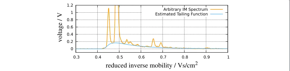
• Every spectrum contains a tailing of the RIP, so the RIP is right-skewed (Figure 2). To extract peaks, the effect of the RIP and its tailing must be estimated and removed.
• At higher concentrations, compounds can form dimer ions, and one may observe both the monomer and dimer peak from one compound. This means that there is not necessarily a one-to-one correspondence between peaks and compounds, and our work focuses on peak detection, not compound identification. • An IM spectrometer may operate in positive or
negative mode, depending on which type of ions (positive or negative) one wants to detect. In either case, signals are reported in positive units. All experiments described here were done in positive mode.
Peak models
For our purpose of analyzing MCC/IMS measurements, a peak is characterized by the following assumptions.
Figure 1Visualization of a raw measurement (IMSC) as a heat map; signal color: white (lowest)<blue<purple<red<yellow (highest). The constantly present reactant ion peak (RIP) with mode at 0.48 Vs/cm2and exemplarily one VOC peak are annotated.
calculated with respect to the mode for each dimension i. At its mode(m1,. . .,mn), peak P exceeds the average back-ground noise level by a certain factor times the standard deviation of the noise.
For MCC/IMS measurements, we haven = 2 dimen-sions, and in both retention time dimension and IRM dimension, we use the shifted Inverse Gaussian distribu-tiong[13] as peak model function:
g(x;μ,λ,o):= 1[√x>o]
2π ·
·
λ
(x−o)3 ·exp
−λ ((2μx−2(o)−μ)2
x−o)
. (1)
Its parameters are the shift (or offset) o, the relative meanμ > 0 (to the right of o) and the shape parame-ter λ > 0. A peak is then given as the product of two shifted Inverse Gaussians, scaled by a volume factorv, i.e., by seven parameters; so the density function of a peak is p(r,t):=v·g(r,μr,λr,or)·g(t,μt,λt,ot)for allr∈R,t∈T. Since the parametersμ,λ,oof a shifted Inverse Gaus-sian may be different even though the resulting distribu-tions have a similar shape, it is more intuitive to describe the shifted Inverse Gaussian in terms of three differ-ent descriptors: the (absolute) mean μ = o + μ, the standard deviationσ and the modem. There is a bijec-tion between(μ,λ,o)and(μ,σ,m) [13] summarized in Appendix A.
We also make use of the following empirically observ-able properties of peaks in real IMSCs that concern the peak widths on both the IRM axis and the retention time axis. The width can be described as the length ω1/2 of the interval around the mode where the peak height is at least half of its maximum height. For a (symmetric) Gaus-sian distribution, there is a linear relation between the standard deviationσandω1/2:
ω1/2=φ·σ withφ =2 √
2 ln 2≈2.3548 . (2)
This relation approximately holds as well for not too skewed Inverse Gaussian distributions and is a good approximation to estimate its descriptorσ approximately from an empirically observedω1/2.
Given the mode d∗ of a peak in drift time (in ms), we can estimate its descriptors (m,σ,μ) in IRM units as follows. Recall that the IRM mode (in V s cm−2) is simply m = Ct|d · d∗, where Ct|d is the conver-sion constant between drift time and IRM (see Section ‘Data from MCC/IMS measurements’). Spangleret al.[14] empirically derived thatω1/2 =
(11.09Dd∗)/v2d+d2grid, whereDis the diffusion coefficient,vdthe drift velocity. Using the Einstein relation [15], Dcan be computed as D= kKBT/q, wherekis the ion mobility,KBthe Boltz-mann constant, T the absolute temperature and q the electric charge. We then use (2) to estimateσ ≈ ω1/2/φ. Finally, the mean is empirically found to be μ ≈ Ct|d ·
d∗+(4.246·10−5)2+(d∗)2/585048.1633.
On the retention time axis, the peak width ω1/2 grows approximately linearly with retention time, i.e.,
there are constants r_width_offset > 0 and
r_width_factor > 0 such that width of a peak with maximum at retention timeris approximately
ξ(r):=r·r_width_factor+r_width_offset. (3)
Optimization methods
The online peak extraction algorithm makes use of non-linear unconstrained minimization, similar to non-non-linear least squares, and of the EM algorithm. Both methods are summarized here.
Non-linear Least Squares
The NLLS method is an iterative method to estimate parameters θ = (θ1,. . .,θq) of a supposed paramet-ric function f, givennobserved data points(x1,y1),. . ., (xn,yn) with yi = f(xi;θ). The idea is to minimize the quadratic error ni=1r2i(θ)between the function and the observed data, whereri(θ):= yi−f(xi;θ)is theresidual of thei-the datapoint. The necessary optimality condition is i ri(θ)·∂ri(θ)/∂θj = 0 for all j. If f is linear in θ (e.g., a polynomial inxwithθ being the polynomial coef-ficients, a setting called polynomial regression), then the optimality condition results in a linear system, which can be solved in closed form. However, oftenf is not linear inθ and we obtain a non-linear system, which is solved iteratively, given initial parameter values, by linearizing it in each iteration. Details and different algorithms for NLLS can be found in the literature ([16], Chapter 10). In this paper, we use a different, non-symmetric loss func-tion, but apply similar techniques to solve the problem (see below).
The EM algorithm for mixtures with heterogeneous components
The observed data x = (x1,. . .,xn) is viewed as a sample from a mixture of probability distributions, where the mixture density is specified by f(xi|ω,θ) =
C
c=1ωc fc(xi|θc). Herecindexes theCdifferent com-ponent distributionsfc, whereθcdenotes the parameters offc, andθ = (θ1,. . .,θC)is the collection of all parame-ters. The mixture coefficients satisfyωc ≥0 for allc, and
cωc = 1. Unlike in most applications, where all com-ponent distributions fc are multivariate Gaussians, here the fc are of different types (e.g., uniform and Inverse Gaussian). The goal is to determine the parametersωand θsuch that the probability of the observed sample is max-imal (maximum likelihood paradigm). Since the resulting optimization problem is non-convex in (ω,θ), the EM algorithm is an iterative method that will converge to a local optimum [17] in parameter space. The EM algorithm
consists of two repeated steps: The E-step (expectation) estimates the expected membership of each data point in each component and then the component weights ω, given the current model parametersθ. The M-step (max-imization) estimates maximum likelihood parametersθc for each parametric componentfcindividually, using the expected memberships as hidden variables that decouple the model.
E-Step. To estimate the expected membership Wi,c of data pointxiin each componentc, the component’s rela-tive probability at that data point is computed, such that
cWi,c = 1 for alli. Then the new component weight estimates ω+c are the averages of Wi,c across all n data points.
Wi,c= ωc
fc(xi|θc)
k ωkfk(xi|θk)
, ω+c = 1 n
n
i=1
Wi,c, (4)
Convergence. After each M-step of an EM cycle, we compare θc,q (old parameter value) and θc+,q (updated parameter value), where q indexes the elements of θc, the parameters of component c. We say that the algo-rithm has converged when the relative change κc,q :=
|θ+
c,q−θc,q|/max
|θ+ c,q|,|θc,q|
drops below a given thresh-old thresh for all c,q, (if θc+,q = θc,q = 0, we set κc,q:=0).
Having reviewed the necessary background, we now describe the methods we use for peak extraction from IMSCs.
Denoising and baseline correction Background
A major challenge during peak detection in an IM spec-trum is to find peaks that only slightly exceed the back-ground noise level in a spectrumS = (St). To determine whether the intensityStat coordinatetbelongs to a peak region or can be solely explained by background noise, we propose a method based on the EM algorithm. It runs inO(τ|T|)time whereτis the number of EM iterations.
Mixture model
Based on observations of IM spectra signal intensities, we assume that
• the noise intensity has a Gaussian distribution over low intensity values with meanμNand standard
deviationσN,
pN(s|μN,σN)=
1 √
2π σN
·exp−(s−μN)2/(2σN2)
• the true signal intensity has an Inverse Gaussian distribution with meanμSand shape parameterλS,
pS(s|μS,λS)=
λS/(2πs3)·exp
−λS(s−μS)2/(2μ2Ss)
• there is an unspecific background component which is not well captured by either of the two previous distributions; we model it by the uniform distribution over all intensities,
pB(s)=1/(max(S)−min(S)),
and we expect the weightωBof this component to be
close to zero in standard IM spectra. High weights indicate an anomaly during the measurement.
We interpret the observed spectrum S as a sample of a mixture of these three components with unknown mixture coefficients. To illustrate this approach, consider Figure 3, which shows the empirical intensity distribution (histogram) of an arbitrary spectrum, together with the estimated components (except the uniform distribution, which has the expected coefficient of almost zero).
It follows that there are six independent parameters to estimate:μN, σN, μS, λS and weights ωN,ωS,ωB (noise, signal, background, whereωB=1−ωN−ωS).
Initial parameter values
Background noise intensities are assumed to follow a Gaussian distribution at small intensity values. We can determine its approximate meanμNand standard devia-tionσNby considering the first and last 10% of data points in each spectrum.
The initial weight of the noise component is set to cover most points covered by this Gaussian distribution, i.e., ωN:= |{t∈T|StμN+3σN}| /|T|.
We assume that almost all of the remaining weight belongs to the signal component, thusωS = (1−ωN)· 0.999, andωB=(1−ωN)·0.001.
To obtain initial parameters for the signal model, let I := {t ∈ T|St > μN + 3σN} (the complement of the intensities that are initially assigned to the noise com-ponent). We setμS = t∈I(St−μN)
/|I|andλS = ( t∈I(1/(St−μN)−1/μS))−1(which are the maximum likelihood estimators for Inverse Gaussian parameters).
E-step
The hidden parameters Wt,c are computed using (4), where the three component distributionsfcare the three component densitiespN,pS,pBwith their parameters and the data x is a mean-smoothed version of the original spectrumS:xt:= 2α1+1· tt+=αt−αSt, where the smoothing window margin isα:=(1/2)·dgrid·Ct|d· |T|/Tlast. (Here dgridis the grid opening time of the spectrometer andTlast is the maximum IRM inT).
Maximum likelihood estimators
In the maximization step (M-step) we estimate maximum likelihood parameters for the non-uniform components using the original intensities ofSagain.
μN= t
Wt,N·St
tWt,N
, (5)
μS= t
Wt,S·(St−μN)
tWt,S
, (6)
σ2
N= t
Wt,N·(St−μN)2
t Wt,N
, (7)
λS= t
Wt,S
t Wt,S·(1/(St−μN)−1/μS)
(8)
for allt∈T.
Final step
After convergence, we correct the baseline and remove noise: We first subtractμNfrom the signal value and then reduce the remaining value by the estimated noise weight. The corrected spectrumS+is
S+t :=max(1−Wt,N)(St−μN), 0
, t∈T.
Reducing a spectrum to peak models Background
The idea of processing a single (noise-reduced) IM spec-trum S is to deconvolute it into separate components described with statistical distribution functions. Several components appear in each spectrum besides the peaks, namely the previously described RIP and the tailing
described in Section ‘Data from MCC/IMS measure-ments’. and background noise. We first determine and remove the RIP tailing function and then determine the peak parameters (including the RIP).
Determining the tailing function
The tailing function appears as a baseline in every spec-trum (see Figure 2 for an example). Its shape and scale changes from spectrum to spectrum; so it has to be deter-mined in each spectrum and subtracted in order to extract peaks from the remaining signal in the next step. Empir-ically, we observe that the tailing function f(t) can be described by a scaled shifted Inverse Gaussian, f(t) = v·g(t;μ,λ,o)withggiven by (1). The goal is to determine the parametersθ = (v,μ,λ,o)such that fθ(t) under-fits the given dataS=(St), as shown in Figure 2.
Let rθ(t) := S(t)− fθ(t) be the residual function for a given choice θ of parameters. As we want to penalize r(t) <0 but not (severely)r(t) >0, we use the following non-symmetric loss function that depends on a threshold parameterγ >0:
et(θ;γ ):=
rθ(t)2/2 ifrθ(t) < γ, γ ·rθ(t)−γ2/2 ifrθ(t)≥γ.
That is, the loss at timetis the residual squared when it has a negative or small positive value less than the given threshold γ > 0, but becomes a linear function of the residual for larger positive residuals.
The goal is to findθ to minimize the total lossL(θ):=
tet(θ;γ ) for the given spectrumS and givenγ > 0. We use gradient descent to solve this nonlinear opti-mization problem, to which we refer as non-linear loss minimization (NLLM).
To estimate the tailing function,
1. we determine reasonable initial values for the parametersθ =(v,μ,λ,o)(see below),
2. we solve NLLM withγ =σN2to estimate the scaling factorv, leaving the other parameters fixed,
3. we solve NLLM withγ =σN2to estimate all four parameters,
4. we solve NLLM withγ =σN2/100to re-estimate the scaling factorv
where σN is the standard deviation of the noise as described in Section ‘Denoising and baseline correction’.
The initial parameter values(v,μ,λ,o)are determined as follows: For the scaling factor, we initially set v = (1/2) t|T| St. For the other parameters, we first esti-mate the descriptors (μ,σ,m) as described below and then use the correspondence to the parameters listed in Appendix A. The initial σ is set to the standard devia-tion of the whole RIP-only spectrum. We determine the initialmas the RIP mode. It is a property of the Inverse
Gaussian distributions under consideration such that the meanμcan only range within the intervalI =[m,m+ 0.7σ]. To obtain an appropriate value for μ, an auxil-iary offset variable o is set to the largest IRM left of the RIP mode where the signal is belowσN, andμ it is increased in small steps withinI. The candidate descrip-tors(μ,σ,m) are converted into corresponding param-eters (μ,λ,o) untilo ≥ o. The so obtained parameters constitute the initial parameter values.
Extracting peak parameters from a single spectrum
To extract all peaks from a spectrum (from left to right), we repeat three sub-steps:
1. scanning for a potential peak, starting where the previous iteration stopped;
2. determining peak parameters (Inverse Gaussian distribution);
3. subtracting the peak from the spectrum and continuing with the remainder.
Scanning. The algorithm scans for peaks, starting at the left end ofS, by sliding a window of a given width acrossS and fitting a quadratic polynomial model to the data points within the window. The window width (in index units) is related to the grid opening timedgridof the spec-trometer and given asdgrid/Dlast· |D|data points, where Dlastis the maximum (last) drift time measured.
The model is built in drift time (not IRM). Letf(d;θ)= θ2d2+θ1d+θ0be the fitted quadratic polynomial inside the window. We call a window a peak window if the following conditions are fulfilled:
• the extreme drift timed∗=θ1/(2θ2)lies within the
drift times of the window;
• the extreme drift timed∗indicates a maximum (i.e., θ2<0);
• the maximum is sufficiently high above the noise level (which is zero after preprocessing):f(d∗;θ)≥σN
The first condition can be more strongly restricted to achieve more reliable results, by shrinking the interval towards the center of the window. If no peak is found, the moving window is shifted one index forward. If a peak is detected, the window is shifted half the window length forward before the next scan begins, but first the peak parameters are computed.
The model function is subtracted from the spectrum, and the next iteration is started with a window shifted byα index units (consider Section ‘E-step’). For each spectrum, the output of this step is aspectrum peak list, which is a set of parameters for a mixture of weighted Inverse Gaussian models describing the peaks.
Aligning consecutive spectrum peak lists Background
Having a set of peak parameters for each spectrum, the question arises how to merge the sets P = (Pi) and P+= (P+j )of two consecutive spectra. For each peakPi, we have stored the Inverse Gaussian parametersμi,λi,oi, the peak descriptorsμi,σi,mi(mean, standard deviation, mode) and the scaling factorvi, and similarly so for the peaksPj+. The idea is to compute a global alignment simi-lar to the Needleman-Wunsch method [18] betweenPand P+. We need to specify how to score aligningPitoP+j and how to score leaving a peak unaligned (i.e., a gap).
Scoring peak alignments
The scoreZijfor aligningPitoP+j is chosen by evaluating Pi’s density function at the new modem+j and compar-ing it to “typical” value an approximate standard deviation away from the mode (atmi+δ, whereδ:=dgrid·Ct|d/φ), resulting in the log-odds score
ζi,j=ln
g(m+j ;μi,λi,oi)
g(mi+δ; μi,λi,oi)
.
Alternatively, leaving a peak unmatched results in a gap score of zero.
Applying Needleman-Wunsch global alignment, we can compute the optimal score of aligning the first i peaks in the former spectrum with the firstjpeaks in the cur-rent spectrum by dynamic programming. We initialize a matrixZ, setting allZi,0andZ0,jto zero and then compute, fori≥1 andj≥1,
Zi,j=max ⎧ ⎨ ⎩
Zi−1,j−1+ζi,j, Zi−1,j, Zi,j−1.
Obtaining peak chains
The alignment is obtained with a traceback, recording the optimal case in each cell, as usual. There are three cases to consider.
• IfP+j is not aligned with a peak inP, potentially a new peak starts at this retention time. Thus modelPj+is put into a new peak chain.
• IfPj+is aligned with a peakPi, the chain containing Piis extended withP+j .
• All peaksPithat are not aligned to any peak inP+ indicate the end of a peak chain at the current retention time.
All completed peak chains are forwarded to the next step, two-dimensional peak model estimation.
Estimating 2-D peak models Background
Let C = (P1,. . .,Pn) be a chain of one-dimensional Inverse Gaussian models. The goal of this step is to esti-mate a two-dimensional peak model (product of two one-dimensional Inverse Gaussians) from the chain, as described in Section ‘Peak models’, or to reject the chain if the chain does not fit such a model well. Potential problems are that a peak chain may contain noisy 1-D peaks truncated at their borders, consist only of noise or in fact consist of several consecutive 2-D peaks at the same drift time and successive retention times.
Estimating the parameters
As discussed in Section ‘Peak models’, the half-height widthω1/2in retention time of a peak centered at retention timercan be described by an affine functionξ(r), Eq. (3), andω1/2can be converted to the corresponding number of data points (window width).
We have the parameters(vˆi,μˆi,t,λˆi,t,oˆi,t)for each indi-vidual peak i = 1,. . .,n in a peak chain, and the corresponding descriptors (μˆi,t,σˆi,t,mˆi,t), as well as the associated retention time ri and peak height hi = ˆvi · g(mˆi,t;μˆi,t,λˆi,t,oˆi,t).
We proceed similarly to Section ‘Extracting peak param-eters from a single spectrum’ by fitting quadratic polyno-mialsb(r;θ) = θ2r2+θ1r+θ0in sliding windows of the appropriate widthξ(ri)such thathi≈b(ri;θ).
Having found a window that fits a peak, we estimate ini-tial descriptors for an Inverse Gaussian model in retention time as follows:
vr= −θ12/(4θ2)+θ0, σr=
vr/(2|θ2|), mr= −θ1/(2θ2),
μr=mr+ξ(mr) / (4φ).
The descriptors are then converted into model parame-ters (see Appendix A).
To obtain the Inverse Gaussian distribution parame-ters in the IRM dimension for each of the k models, we first compute model descriptors using a membership-weighted average over the individual model descriptors: Forj∈ {1,. . .,k}, let
Mj:=
in Mi,j,
μj,t:= 1 Mj
in
Mi,j· ˆμi,t,
σj,t:= 1 Mj
in
Mi,j· ˆσi,t,
mj,t:= 1 Mj
in
Mi,j· ˆmi,t.
We then convert these descriptors back into model parameters (Appendix A). The final peak volume is com-puted asv∗j =vj,r· invi,t.
For every modelj ∈ {1,. . .,k}, we check the following conditions:
• The width at half height in the retention time dimension has approximately the expected size (cf. Eqs. (2), (3)):ξ(mj,r)/2σj,r/φ <2·ξ(mj,r), • The peak height at its maximum is sufficiently above
the noise level:v∗j ·g(mj,t;μj,t,λj,t,oj,t)·
g(mj,r;μj,r,λj,r,oj,r)≥noise_margin·σN, where noise_margin>0is a tunable parameter, • the Inverse Gaussian peak modelgin retention time
correlates well (in terms of the Pearson
product-moment correlation coefficientρ) with its quadratic approximationbin a window around the mode. More precisely, consider the window
W=[mj,r−ξ(mj,r)/φ, mj,r+ξ(mj,r)/φ], the model
vectorG=g(x;μj,r,λj,r,oj,r)forx∈Wand the
quadratic approximation vectorB=bj(x;θ)for x∈W, and test whether the Pearson correlation satisfiesρ(G,B)≥ρmin.
If all conditions are satisfied, we have identified a 2-D peak model (v∗j,μj,t,λj,t,oj,t,μj,r,λj,r,oj,r). Otherwise the model is discarded.
Peak clustering Background
We now consider a series of IMS measurements, for each of which we have extracted peaks available in the form of parameter vectors or descriptors. The question arises how to decide which descriptors in different measurements represent the same peak (and hence potentially the same VOC).
Let X be the union of peak locations in all mea-surements, let |X| =: n, and let Xi,R be the reten-tion time of peak i and Xi,T its IRM. We introduce a clustering approach using the EM algorithm with two-dimensional Gaussian mixtures that differs from the stan-dard approach by its ability to dynamically adjust the number of clusters in the process.
Mixture model
We assume that the measured retention times and IRMs belonging to peaks from the same compound are indepen-dently normally distributed in both dimensions around the (unknown) true retention time and IRM. Let θj := (μj,R,σj,R,μj,T,σj,T) be the parameters for component j, and letfj(xgivenθj be a two-dimensional Gaussian prod-uct distribution for a peak locationx=(xR,xT)with these parameters.
The mixture distribution isf(x)= Cj=1ωjfj(x|θj)with a yet undetermined numberCof clusters. Note that there is no “background” model component.
Initial parameter values
In the beginning, we initialize the algorithm with as many clusters as peaks, i.e., we set C := n. This assignment makes a background model obsolete, because all peaks are assigned to at least one cluster. All clusters get as start parameters forμj,R,μj,T the original retention time and IRM of peak locationXj, respectively, forj=1,. . .,n. We setσj,T:=t_width>0 andσj,R :=ξ(Xj,R)/φ.
Dynamic adjustment of the number of clusters
After computing weights in the E-step, but before starting the M-step, we dynamically adjust the number of clusters by merging clusters whose centers are close to each other. Every pairj < kof clusters is compared in a nested for-loop. When|μj,T−μk,T|<t_widthand|μj,R−μk,R|< ξmax{μj,R,μk,R}
, then clusters j andk are merged by summing the EM weights: ω+ := ωj +ωk andWi,+ := Wi,j +Wi,k for alli. The summed weights are assigned to the location of the cluster with larger weight. (The re-computation of the parameters happens immediately after merging in the maximization step). The comparison order may matter in rare cases for deciding which peaks are merged first, but since new means and variances are com-puted, possible merges that were omitted in the current iteration will be performed in the next iteration.
This merging step is applied after in the second EM iter-ation, since the cluster means need at least one iteration to move towards each other.
Maximum likelihood estimators
μj,d= n
i=1Wi,j·Xi,d n
i=1Wi,j
, d∈ {T,R}, (9)
σ2 j,d=
n
i=1Wi,j·(Xi,d−μj,d)2 n
i=1Wi,j
, d∈ {T,R}, (10)
for all componentsj=1,. . .,C.
One problem using this approach emerges from the fact that initially each cluster contains only one peak, leading to an estimated variance of zero in many cases. To pre-vent this, minimum values are enforced such thatσj,T ≥
t_widthandσj,R≥ξ(μj,R)/φfor allj.
Final step
The EM loop terminates when no merging occurs and the convergence criteria for all parameters are fulfilled. The resulting membership weights determine the number of clusters as well as the membership coefficient of peak locationXito clusterj. If a hard clustering is desired, the merging step has to be traced.
Evaluation
We evaluate different properties of the online method:
1. the quality of reducing a single spectrum to a peak list (denoising/baseline correction (Section ‘Denoising and baseline correction’) and spectrum reduction (Section ‘Reducing a spectrum to peak models’), 2. the execution time of both steps,
3. the quality of the new clustering approach,
4. the correlation between manual annotations on full IMSCs by a computer-assisted expert and our automated online extraction method.
Parameters. For evaluation measurements, the MCC was adjusted to a temperature of 40°C and throughput of 150 mL min−1. The IMS had a voltage of 4380 V, a grid opening time of 300μs and a throughput of 150 mL min−1. We chose the following parameters [9]:
• r_width_offset= 2.5 s (width offset for peaks in retention time),
• r_width_factor= 0.06 (width slope for peaks in retention time),
• t_width= 0.003 V s cm−2(standard deviation for peaks in IRM),
• thresh(convergence threshold; value varies within evaluation),
• noise_margin= 4 (factor multiplied with standard deviation of background noise for minimal peak height),
• ρmin= 0.95 (minimal Pearson product-moment correlation coefficient).
Quality of single spectrum reduction
In a first experiment, we tested the quality of the spec-trum reduction method using an idea by Munteanu and
Wornowizki [19] that determines the agreement between an observed set of data points, interpreted as an empirical distribution functionF (the data) and a model distribu-tionG(the mixture distribution obtained from the peak list parameters). The approach writesF= ˜s·G+(1−˜s)·H with˜s ∈[ 0, 1], whereHis a non-parametric distribution whose inclusion ensures the fit of the model G to the dataF. If the weight˜sis close to 1.0, thenF is a plausi-ble sample fromG. We compare the original spectra and reduced spectra (peaks from peak lists) from a previously used dataset [20]. This set contains 69 measurements preprocessed with a 5×5 average. Every measurement contains 1200 spectra. For each spectrum in all measure-ments, we computed the reduced spectrum model and determineds˜. Over 92% of all 82 000 models achieved˜s= 1 and over 99% reached˜s≥0.9. No˜sdropped below 85%. In summary, spectrum reduction provides an accurate parametric representation of most spectra.
Execution time
We tested our method on two different platforms, (1) a desktop PC with Intel(R) Core(TM) i5 2.80GHz CPU, 8GB memory, Ubuntu 12.04 (64bit) OS and (2) a Rasp-berry Pi [21] type B with ARM1176JZF-S 700MHz CPU, 512 MB memory, Raspbian Wheezy (32bit) OS, once with the factory defaults of 700 MHz and once overclocked up to 900 MHz. The Raspberry Pi was chosen because it is a complete credit-card-sized low-cost single-board com-puter with low CPU and power consumption (3.5 w). This kind of device is appropriate for data analysis in future mobile measurement devices.
Recall that each spectrum contains 12 500 data points. It is current practice to analyze not the full spectra, but aggregated ones, where five consecutive values are aver-aged. Here we consider the full spectra, slightly aggregated ones (average over two values, 6 250 data points) and standard aggregated ones (average over five values, 2 500 data points). We measured the average execution time of denoising, baseline correction and consecutive spectrum reduction. Table 1 shows the results. It is remarkable that at the highest resolution (Average 1) the Raspberry Pi with 900 MHz keeps barely the time bound of 100 ms between consecutive spectra. At lower resolutions, the Raspberry Pi satisfies the time restrictions easily. The desktop PC copes with the analysis effortless on any setting.
Table 1 Average processing time of denoising, baseline correction and spectrum reduction on two platforms with different clock rates, averaging methods (single spectra, averages of 2 and 5 spectra) and convergence thresholds
thresh
thresh Platform Avg 1 Avg 2 Avg 5
0.1%
Desktop PC 4.36 ms 2.09 ms 0.88 ms
Rasp. Pi (700 MHz) 119.48 ms 55.02 ms 21.82 ms
Rasp. Pi (900 MHz) 97.19 ms 43.62 ms 17.42 ms
1.0%
Desktop PC 4.26 ms 2.01 ms 0.66 ms
Rasp. Pi (700 MHz) 116.69 ms 52.63 ms 16.99 ms
Rasp. Pi (900 MHz) 94.03 ms 41.46 ms 13.48 ms
Clustering
To evaluate peak clustering methods, we simulate peak locations according to locations in real MCC/IMS datasets, together with the true partitionPof peaks.
Most of the detected peaks appear in a small dense area early in the measurement. The remaining peaks are dis-tributed widely, which is referred to as the sparse area (we let the areas overlap such that the dense are is contained in the sparse area). The areas approximately have the fol-lowing boundaries (in units of (V s cm−2, s) from lower left to upper right point, cf. Figure 1:
measurement:(0, 0),(1.45, 600) dense area:(0.5, 4),(0.7, 60) sparse area:(0.5, 4),(1.2, 450)
Peak clusters are ellipsoidal and dense. From [9], we know the minimum required distance between two peaks in order to be identified as two separate compounds. We simulate 30 peak cluster centroids in the dense area and 20 in the sparse area, all picked randomly and uniformly distributed in the respective area. We then randomly pick the number of peaks per cluster. We also randomly pick the distribution of peaks within a cluster. Since we do not know the actual distribution model, we decided to sim-ulate with three models: normal (n), exponential (e) and uniform (u) distribution with the following densities:
fn(r,t|μt,σt,μr,σr)
=N(t|μt,σt)·N(r|μr,σr) fe(r,t|μt,λt,μr,λr)
=λtλrexp
−(λt|t−μt| +λr|r−μr|)
/4 fu(r,t|μt,νt,μr,νr)
=
(πνtνr)−1 if|t−μt|
2
ν2
t +
|r−μr|2
ν2
r 1
0 otherwise
Here(μt,μr)is the coordinate of the centroid with RIM in Vs/cm2and retention time in s. For the normal distri-bution, we usedσt=0.002 andσr =μr·0.002+0.2. For the exponential distribution, we usedλt=(1.45·2500)−1
(reduced mobility width for in single cell withinM) and λr = 1/(μr ·0.002+0.2). For the uniform distribution, we used an ellipsoid with radii νt = 0.006 and νr = μr·0.02+1.
We compared our adaptive EM clustering with two common clustering methods: k-means and DBSCAN. Since k-means needs a fixed number of clusters k and appropriate start values for the centroids, used k -means++ [22] for estimating good starting values and give it an advantage by assigning the true number of parti-tions. DBSCAN has the advantages that it does not need to know the number of clusters in advance and that it can find non-linear cluster boundaries, but it does not easily yield parametric cluster descriptors.
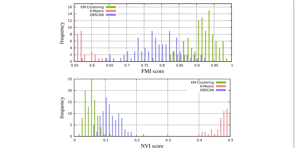
To measure the quality of an obtained clustering C we use the Fowlkes-Mallows index (FMI, [23]) and the normalized variation of information (NVI) score [24].
For the FMI one considers all pairs of data points. If two data points belong to the same true partition ofP, they are called connected. Accordingly, a pair of data points is called clustered if they are clustered together by the clustering method are evaluating. Pairs of data points that are both connected and clustered are called true positives (TP). False positives (FP, not connected but clustered) and false negatives (FN, connected but not clustered) are computed analogously. The FMI is the geometric mean of precision and recall: FMI(P,C) := √
TP/(TP+FP)·TP/(TP+FN), where P is the true partition and C is the clustering. We have FMI(P,C) ∈ [ 0, 1], and FMI(P,C) = 1 indicates perfect agreement. The FMI is difficult to interpret when the number of clusters inCandPdiffers significantly.
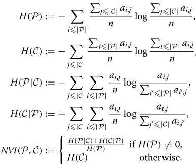
Therefore we use a second measure that considers clus-ter sizes only, the normalized variation of information (NVI). To compute the NVI, an auxiliary (|P| × |C| )-dimensional matrix A = (ai,j) is computed, where ai,j is the number of data points within partition i that are assigned to cluster j. The NVI score is defined via entropies; letnbe the number of data points and
H(P):= − i|P|
j|C|ai,j
n log
j|C|ai,j
n ,
H(C):= − j|C|
i|P|ai,j
n log
i|P|ai,j
n ,
H(P|C):= − j|C|
i|P| ai,j
n log ai,j
i|P|ai,j ,
H(C|P):= − j|C|
i|P| ai,j
n log ai,j
j|C|ai,j ,
NVI(P,C):=
H(P|C)+H(C|P)
H(P) ifH(P)=0,
Figure 4Histograms of Fowlkes-Mallows index (FMI; higher is better) and normalized variation of information (NVI; lower is better) comparing 100 simulated measurements containing partitioned peak locations with their clusters produced by the different methods.
Here NVI(P,C) = 0 indicates perfect agreement between the cluster size distributions. Together, an FMI of 1 and an NVI score of 0 indicate a perfect clustering.
For the first test, we evaluated 100 sets of data points distributed as described above. The cluster model (nor-mal, exponential or uniform) was drawn randomly. The
results show that even with the advantage thatk-means knows the true k, our adaptive EM clustering performs best on average in terms of FMI and NVI score (Figure 4). For the second test, we additionally inserted 200 uni-formly distributed (noise) peaks into the measurement area. All these peaks are singletons and have no matching
Figure 6Time series of discovered intensities of two peaks. Left: A peak with agreement between manual and automated online annotation. Right: A peak where the online method fails to extract the peak in several measurements. If one treated zeros as missing data, the overall trend would still be visible.
peaks. The results (Figure 5) show that the adaptive EM clustering still performs best on average, whereask-means fails.
Comparison of automated online peak extraction with manual offline annotation
The fourth experiment compares extracted peaks from a time series of measurements of two automated methods to an expert manual annotation. The automated methods are our online analysis process described here and auto-mated peak detection using the commercial VisualNow software.
Here 15 rats were monitored in 20 minute intervals for up to a day. Each rat resulted in 30–40 measure-ments (a time series) for a total of 515 measuremeasure-ments. To track peaks over time, we used the previously described EM clustering method.
As an example, Figure 6 shows time series of intensi-ties of two peaks detected by computer-assisted manual annotation and using our online algorithm. The exam-ple shows that there are cases where the sensitivity of the online algorithm is not perfect; this is mainly true for peaks whose intensity only slightly exceeds the back-ground noise.
To obtain an overview over all time series, we com-puted the cosine similarity γ ∈[−1,+1] time series of peak intensities discovered by manual annotation and each automated method. We also computed the recall automated method for each time series, that is, the rela-tive fraction of measurements where the peak was found by the algorithm among those where it was found by manual annotation. Figure 7 shows overall good agree-ment between both automated methods (our online method and automated VisualNow peak extraction) with
the expert manual annotation. The cosine similarity of the inferred time series is in better agreement than the more variable recall. When comparing automated meth-ods against each other, we outperform VisualNow in terms of sensitivity and computation time: About 31% of the points extracted by the online method exceed 90% recall and 98% cosine similarity whereas only 5% of the time series extracted by VisualNow achieve these values. The peak detection of one measurement takes about 2 seconds on average (when the whole measurement is available at once) with the online method and about 20 seconds with VisualNow on the desktop computer described above. VisualNow only provides the position and signal intensity of the peak’s maximum, whereas our method additionally provides shape parameters.
Problems of our online method stem from low-intensity peaks only slightly above the detection threshold, and resulting fragmentary or rejected peak chains.
Discussion and conclusion
We presented the first approach to extract peaks from MCC/IMS measurements while they are being captured, with the long-term goal to remove the need for storing full measurements before analyzing them in small embedded devices. Our method is fast and satisfies the time restric-tions even on a low-power CPU platform like a Raspberry Pi and outperforms existing software.
While performing well on single spectra, there is room for improvement in merging one-dimensional peak mod-els into two-dimensional peak modmod-els. Our method has to be further evaluated in clinical studies or biotechnologi-cal monitoring settings. It also has not been tested with the negative mode of an IMS for lack of data. In general, the robustness of the method under adversarial condi-tions (high concentracondi-tions with formation of dimer ions, changes in temperature or carrier gas flow in the MCC) has to be evaluated and probably improved.
Appendix A: peak descriptors and parameters The shifted Inverse Gaussian distribution with parameters o(shift or offset),μ(mean minus shift, also called relative mean) and λ (shape) is given by (1). There is a bijec-tion [13] between(μ,λ,o)and the descriptors(μ,σ,m), which are the absolute meanμ = o+μ, the standard deviationσand the modem. Given(μ,λ,o), we have
μ=μ+o, σ =μ3/λ,
m=μ·1+(9μ2)/(4λ2)−(3μ)/(2λ)+o,
and, given(μ,σ,m), we use auxiliary expressionspandq to find
p:=−m(2μ+m)+3·(μ2−σ2)/2(m−μ),
q:=m(3σ2+μ·m)−μ3/2(m−μ),
o= −p/2−
p2/4−q, μ=μ−o,
λ=μ3/σ2.
Competing interests
The authors declare that they have no competing interests.
Authors’ contributions
DK developed and implemented the methods and evalutated them in consultation with SR. DK and SR wrote the manuscript. Both authors read and approved the final manuscript.
Acknowledgements
DK and SR acknowledge the support of Deutsche Forschungsgemeinschaft (DFG) within the Collaborative Research Center SFB 876 (http://sfb876.tu-dortmund.de), “Providing Information by Resource-Constrained Data Analysis”, subproject TB1. We are grateful to Jörg Ingo Baumbach for help with numerous questions and for providing datasets. We thank Max Wornowizki from subproject C3 for providing methodology for the first evaluation.
Received: 20 March 2015 Accepted: 2 April 2015
References
1. Bessa V, Darwiche K, Teschler H, Sommerwerck U, Rabis T, Baumbach JI, et al. Detection of volatile organic compounds (VOCs) in exhaled breath of patients with chronic obstructive pulmonary disease (COPD) by ion mobility spectrometry. Int J Ion Mobility Spectrom. 2011;14:7–13. 2. Bunkowski A, Bödeker B, Bader S, Westhoff M, Litterst P, Baumbach JI.
MCC/IMS signals in human breath related to sarcoidosis – results of a feasibility study using an automated peak finding procedure. J Breath Res. 2009;3(4):046001.
3. Westhoff M, Litterst P, Freitag L, Urfer W, Bader S, Baumbach JI. Ion mobility spectrometry for the detection of volatile organic compounds in exhaled breath of lung cancer patients. Thorax. 2009;64:744–8. 4. Keller T, Schneider A, Tutsch-Bauer E, Jaspers J, Aderjan R, Skopp G. Ion
mobility spectrometry for the detection of drugs in cases of forensic and criminalistic relevance. Int J Ion Mobility Spectrom. 1999;2(1):22–34. 5. Ewing RG, Atkinson DA, Eiceman GJ, Ewing GJ. A critical review of ion
mobility spectrometry for the detection of explosives and explosive related compounds. Talanta. 2001;54(3):515–29.
6. Kolehmainen M, Rönkkö P, Raatikainen O. Monitoring of yeast fermentation by ion mobility spectrometry measurement and data visualisation with self-organizing maps. Anal Chim Acta. 2003;484(1):93–100.
7. Kreuder AE, Buchinger H, Kreuer S, Volk T, Maddula S, Baumbach J. Characterization of propofol in human breath of patients undergoing anesthesia. Int J Ion Mobility Spectrom. 2011;14:167–75.
8. Bunkowski A. MCC-IMS data analysis using automated spectra processing and explorative visualisation methods. PhD thesis: Bielefeld University; 2011.
9. Bödeker B, Vautz W, Baumbach JI. Peak finding and referencing in MCC/IMS-data. Int J Ion Mobility Spectrom. 2008;11(1):83–7. 10. D’Addario M, Kopczynski D, Baumbach JI, Rahmann S. A modular
computational framework for automated peak extraction from ion mobility spectra. BMC Bioinformatics. 2014;15(1):25.
11. Kopczynski D, Rahmann S. An online peak extraction algorithm for ion mobility spectrometry data. In: WABI. Lecture Notes in Computer Science. New York: Springer; 2014. p. 232–46.
12. Eiceman GA, Karpas Z. Ion Mobility Spectrom, Second Edition. New York: Taylor & Francis; 2005.
14. Spangler GE, Collins CI. Peak shape analysis and plate theory for plasma chromatography. Anal Chem. 1975;47(3):403–7.
15. Einstein A. Über die von der molekularkinetischen Theorie der Wärme geforderte Bewegung von in ruhenden Flüssigkeiten suspendierten Teilchen. Annalen der Physik. 1905;322(8):549–60.
16. Nocedal J, Wright SJ. Numerical Optimization, 2nd edn. New York: Springer; 2006.
17. Dempster AP, Laird NM, Rubin DB. Maximum likelihood from incomplete data via the EM algorithm. J R Stat Soc Ser B (Methodological).
1977;39:1–38.
18. Needleman SB, Wunsch CD. A general method applicable to the search for similarities in the amino acid sequence of two proteins. J Mol Biol. 1970;48(3):443–53.
19. Munteanu A, Wornowizki M. Demixing empirical distribution functions. Technical Report 2014-02, Collaborative Research Center 876, TU Dortmund. 2014.
20. Hauschild AC, Kopczynski D, D’Addario M, Baumbach JI, Rahmann S, Baumbach J. Peak detection method evaluation for ion mobility spectrometry by using machine learning approaches. Metabolites. 2013;3(2):277–93.
21. Raspberry Pi Foundation. Raspberry Pi. 2014. http://www.raspberrypi.org/. 22. Arthur D, Vassilvitskii S. K-means++: The advantages of careful seeding.
In: Proceedings of the Eighteenth Annual ACM-SIAM Symposium on Discrete Algorithms. SODA ‘07. Philadelphia: Society for Industrial and Applied Mathematics; 2007. p. 1027–35.
23. Fowlkes EB, Mallows CL. A method for comparing two hierarchical clusterings. J Am Stat Assoc. 1983;78(383):553–69.
24. Reichart R, Rappoport A. The nvi clustering evaluation measure. In: Proceedings of the Thirteenth Conference on Computational Natural Language Learning. Stroudsburg, PA, USA: Association for Computational Linguistics; 2009. p. 165–73. http://dl.acm.org/citation.cfm?id=1596374. 1596401.
Submit your next manuscript to BioMed Central and take full advantage of:
• Convenient online submission
• Thorough peer review
• No space constraints or color figure charges
• Immediate publication on acceptance
• Inclusion in PubMed, CAS, Scopus and Google Scholar
• Research which is freely available for redistribution