On the Occasion of his 75th Birthday Anniversary PJSOR, Vol. 8, No. 3, pages 491-506, July 2012
Linking Diversity and Disparity Measures
Sahadeb Sarkar
Operations Management Group
Indian Institute of Management Calcutta Post Box 16757, Calcutta 700 027, India [email protected]
Ayanendranath Basu
Bayesian and Interdisciplinary Research Unit Indian Statistical Institute
203 B. T. Road, Calcutta 700 108, India [email protected]
Abstract
The purpose of this paper is to examine links between the diversity measures (Patil and Taillie 1982) and the disparity measures (Lindsay 1994), quantities apparently developed for somewhat different purposes. We demonstrate that numerous diversity measures satisfying all the desirable criteria mentioned by Patil and Taillie can be defined by the generating functions of certain disparities and the associated residual adjustment functions. This provides the statistician and the ecologist a wide class of flexible indices for the statistical measurement of diversity.
Keywords and phrases:Divergence; Hellinger distance; Negative exponential disparity; Residual adjustment function; Species rarity.
1. Introduction
The statistical measurement of diversity is an extremely important practical problem. Diversity, under various names, has been a very significant concept in ecological, biological, economic, social, physical and management sciences. See Atkinson (1970), Finkelstein and Friedberg (1967), Greenberg (1956), Hart (1971), Lieberson (1969), Nei (1973), and Sen (1974), among others. There is a vast literature on diversity related issues. Here we discuss only some of the important, relevant references.
Two widely used indices of diversity are Shannon's (1948) index and Simpson's (1949) index. Good (1953) suggested a more general diversity measure which includes Shannon's and Simpson's indices. Baczkowski et al. (1997, 1998, 2000) discussed a further generalization of the Good's index.
bio-diversity (Solow and Polasky 1994; Champely and Chessel 2002). Rao (1982a, b) extended the concept of analysis of variance (ANOVA) to the more general analysis of diversity (ANODIV), which can be used for qualitative data as well. His work generalized the work on the analysis of one-way classified categorical data, called CATANOVA, of Light and Margolin (1971) and Anderson and Landis (1980). Nayak (1986a) discussed generalization of the CATANOVA methods of these authors using Rao's quadratic entropy. For a general class of diversity measures, Nayak (1986b) discussed sampling distributions of quantities arising in ANODIV.
In this paper, however, we restrict our attention to the the widely accepted traditional approach of measuring ecological diversity, in which one considers the relative abundances in a community without regard to the differences between species. For this approach, Patil and Taillie (1982) provided a formal definition and logical development of diversity as a concept and worked out a related theory for the statistical measurement of diversity. They defined diversity of a community as the average rarity of species within the community, and proposed a family of measures called diversity indices of degree. Below we mention some recent works on the application of these diversity indices.
For square contingency tables having nominal categories, Tomizawa (1994) proposed two measures to represent the degree of departure from symmetry using the average of the Shannon's index and the average of Simpson's index respectively. Tomizawa et al (1998) gave a generalization of the two measures using the average of the diversity index of Patil and Taillie (1982, Sec 3.2).
For a two-way contingency table with nominal explanatory and a nominal response variable, Tomizawa et al (1997) defined measures which describe the proportional reduction in variation from the marginal distribution to the conditional distributions of the response using Patil and Taillie's (1982) diversity index. Tomizawa and Ebi (1998) extended Tomizawa et al's work to multi-way contingency tables.
In the context of developing robust and fully efficient inference procedures under count data models, Lindsay (1994) defined a class of density based divergences, called disparities. A disparity is a measure of average discrepancy between two densities, which in statistical inference are the model density and an appropriate nonparametric density estimator obtained from the sample data. Lindsay's class of disparities includes the well known and well studied Hellinger distance (HD), the more recent negative exponential disparity (NED) which is an excellent competitor to the HD in generating robust statistics (see Basu et al. 1997), the Pearson's chi-square, the likelihood disparity, and the Kullback-Leibler divergence. This class of disparities contains some important subclasses, namely the blended weight chi-squares, the blended weight Hellinger distances (Lindsay 1994), and the celebrated power divergence family (Cressie and Read 1984).
which the traditional robust estimators such as the M-estimators fail to do. Among others, Tamura and Boos (1986) and Simpson (1987, 1989) further pursued Beran's work. Lindsay (1994) presented a comprehensive approach, developed the class of disparities, and extended the range of choice beyond the Hellinger distance. Many new members of the class of disparities share and sometimes improve upon the desirable properties of the Hellinger distance.
Several disparity based analogs (Simpson 1989, Bhandari et al 2000) of the likelihood ratio test are excellent robust alternatives to the usually non-robust likelihood ratio test. As another application of disparities, Basu and Sarkar (1994) investigated disparity based goodness-of-fit tests for multinomial models under simple as well as composite hypotheses thus generalizing the Cressie-Read power divergence approach. This line of research is pursued by Shin et al (1995, 1996) and Jeong and Sarkar (2000) among others. Thus a considerable amount of research are based on the disparities in the area of robust inference and goodness-of-fit tests. For a comprehensive description see Basu et al (2011).
The form of the diversity index of degree defined by Patil and Taillie (1982) is strikingly similar to that of the well-known power divergence of Cressie and Read (1984). This makes one wonder about possible connections. More generally, since diversity of a community is about measuring the average rarity of its species, and disparity is about measuring the average discrepancy between suitable densities, the question arises: Is there a link between diversity and disparity measures? For example, can one generate diversity measures using the functions related to disparities? Such enquiries motivated the work of the present paper and we hope that we have presented at least a partial answer to the above questions.
The rest of the paper is organized as follows: A short review of diversity measures is given in Section 2 whereas a brief discussion of disparities is provided in Section 3. Section 4 presents the links between diversity and disparity measures. Finally, Section 5 contains some concluding remarks.
2. Diversities
We briefly review the diversity measures introduced by Patil and Taillie (1982). Suppose a certain quantity is distributed among a countable set of categories, labeled i= 1, 2, , with i as the proportionate share received by category i and
ii = 1. This quantitymay be discrete (e.g. biological organisms, errors in a bank ledger) or continuous (e.g. biomass, energy, income).
For concreteness of further discussion on the concept and measurement of diversity, Patil and Taillie consider a community of biological organisms grouped into species and call
finite. A community is called completely even when # # # 1 = 2 = = s = 1/s
, where
# #
1 2
are obtained by arranging the components of in a decreasing order.
Given a community C= ( ,s ), let R i( ; ) denote a numerical measure of rarity to be associated with species i, i= 1,2,. Then a diversity measure of the community is an average rarity of its species, and the diversity indexassociated with the measure of rarity
R is defined by = ( ) = (C ) =
iiR i( ;). Obviously, the diversity measure depend on the choice of the function R measuring rarity of species within the community.Assume that the rarity measure R i( ;) depends only on the numerical value of i. This
phenomenon is called dichotomy, and the resulting diversity index ( )C is known as dichotomous. We will write R i( ;) simply as ( )R i .
Note that the function R measuring rarity is defined on the interval (0,1] and R(0) is inherently undefined and R(1) = 0 is a natural normalizing requirement. Since rarer species correspond to smaller values of , R( ) should be a decreasing function of . Since R(1) = 0, the function R should be nonnegative. Patil and Taillie (1982) listed these conditions in their Criterion C1.
One obtains three widely used indices of ecological diversity 1
0
1
S : = ( ) = 1,
S : = ( ) = log ( ),
S : = ( ) = (1 ),
i i
i
i i i e i
i
i i i i
i
pecies Count R s
hannon Index R
impson Index R
using
( ) = (1i i) / , a ( ) =i i loge( ), ( ) = (1i i i)
R nd R R (1)
respectively. All three assign diversity value zero to a single-species community. The above three measures are special cases of the diversity index of degree, denoted by and defined by
1 1
1
=
( ) = 0, log
i i
i e i
i
if
if
(2)1 1
( ) =
( ) = 0. loge if R if (3)
Note that 0 = lim0. The R functions in equation (1) correspond to = 1,0 and 1 respectively under this setup.
Patil and Taillie imposed another desirable condition on the diversity measures through their Criterion C2: For two communities C= ( ,s ) and C' = ( ,s' '), ( ) C ( )C'
whenever C leads to C' by introducing a species or by a transfer of abundance, which
are defined in the following.
Definition: The community C= ( ,s ) is said to lead to C' = ( ,s' ') by introducing a
speciesif s' =s1 and if there are two distinct positive integers i and j such that , = = = k ' k i
if k i j h if k i h if k j
where 0 < < .h i On the other hand, the community C is said to lead to C' by a
transfer of abundance if s s= ' and if there are positive integers i and j such that
> > 0
i j
and
, = = = k ' k i j
if k i j
h if k i
h if k j
where 0 < <h i j.
To state conditions under which a diversity index ( )C satisfies their Criteria C1 and C2, Patil and Taillie defined an auxiliary function V by
0 = 0
( ) = ( ) 0 < 1. if
V R if
The function V may be discontinuous at 0 . Then, the Criteria C1-C2are satisfied if the auxiliary function V is concave on the closed interval [0,1]. Thus, the diversity index
satisfies Criterion C1 for all and satisfies Criteria C1-C2if 1.
condition comes from the consideration that the diversity in a mixture of populations should not be smaller than the average of diversities within individual populations (Rao 1982b, Sec 2). Criterion C3 is satisfied by a diversity measure if the corresponding auxiliary function V is concave on the closed interval [0,1], and, in particular, by if
1
.
3. Disparities
We very briefly discuss the concept of disparity under count data models. For a detailed discussion see Lindsay (1994) and Basu et al (2011). Let X X1, , ,2 Xn represent a
random sample from a discrete distribution modelled by F having a countable support,
p
IR
. Consider the empirical density estimate d xn( ) = the proportion of Xj's
having the value x. For a value x, Lindsay referred to the normalized deviation between ( )
n
d x and f x( ), given by ( ) = ( ( ) x d xn f x( )) / ( )f x as the Pearson residual( )x , the normalizing being done with respect to the model density. An x-value is called an outlierif it has a large positive Pearson residual ( )x , and it is called an inlierif ( )x is negative.
Let G( ) be a real-valued, convex function on [ 1, ) with G(0) = 0. Then the disparity
G
between dn and f is defined as
( , ) = ( ( )) ( ).
G n
x
d f G x f x
(4)The measure G( , )d fn represents the average discrepancy between dn and f where
the discrepancy (( ( )G d xn f x( )) / ( ))f x is nothing but a suitably modified normalized deviation between d xn( ) and f x( ), and the averaging is done with respect to the model density f. The well-known Cressie-Read power divergence family, indexed by a real parameter , is defined by
[ ( ) / ( )] 1
( , ) = ( )
( 1)
n
n n
x
d x f x PD d f d x
and generated with
1
( 1) 1
( ) =
( 1) G
(5)
where for = 0, 1 , the disparity is defined by continuity, i.e., ( ) = (G 1)loge(1) for = 0 and ( ) =G loge( 1) for = 1 .
The minimizer of (4) with respect to (w.r.t.) is called the minimum disparity estimator (MDE) corresponding to the disparity G. The maximum likelihood estimator (MLE)
of minimizes the likelihood disparity
( )
( , ) = ( )log ( ( ) ( )) , ( )
n
n n n
x
d x
LD d f d x f x d x
f x
with GLD( ) = ( 1)log( 1) . The minimum Hellinger distance estimator (MHDE) minimizes
1/2 1/2 2
( , ) = 2 (n n ( ) ( )) ,
x
HD d f
d x f x with ( ) = 2[( 1)1/2 1] .2HD
G The minimum negative exponential disparity estimator (MNEDE) corresponds to GNED( ) = exp( ) 1 .
Let a x a x( ), ( ) denote the first and second derivatives of a function a x( ) w.r.t. its
argument. Letting denote the gradient w.r.t. , the minimum disparity estimating equation, under differentiability of the model, takes the form
= ( ( )) ( ) = 0,
G x
A x f x
(6) where( ) ( 1) ( )' ( ) A G G (7)
is an increasing function on [ 1, ) . Without changing the estimating properties of the disparity , the function G( ) can be redefined so that
(0) = 0, (0) = 0, ' (0) = 1''
G G and G
retaining its convexity on [ 1, ) , and the corresponding ( ) = (A 1) ( )G' G( ) satisfies A(0) = 0 and A'(0) = 1 in addition to A being increasing on [ 1, ) . When thus standardized, the function A( ) is called the residual adjustment function(RAF) of the disparity.
For the power divergence family, the RAF on [ 1, ) is given by 1
( 1) 1
( ) = .
1
A
(8)
For the LD, HD, and the NED, the RAFs are given by
( ) = , ( ) = 2[ ( 1) 1], a ( ) = 2 (2 ) .
LD HD NED
A A nd A e
The RAF plays a major role in determining the second order efficiency and robustness of the MDEs. The RAF of a disparity controls the impact of large outliers much in the same way as the function of the M -estimation procedure. For an extensive discussion, see Lindsay (1994), Basu and Lindsay (1994) and Basu et al (2011).
4. Links between diversities and disparities
The Criteria C1-C3 of Patil and Taillie (1982) for a diversity measure are satisfied if the corresponding rarity function R( ) defined on the interval (0,1] is:
(i) non-negative, (ii) decreasing, and (iii) have R(1) = 0;
To define either (a) R( ) (and hence V( ) = R( )), or (b) V( ) (and hence ( ) = ( ) /
R V ) satisfying the four properties (i)-(iv), one may use the disparity generating function G or the associated residual adjustment function A on the interval [ 1,0] or [0,1]. We present four cases depending on three factors, namely, whether the function G or A is non-negative or non-positive, increasing or decreasing, and convex or concave on the interval [ 1,0] or [0,1]. Assume that the first and second derivatives of G and A are well defined on [ 1,0] or [0,1].
Case 1. Suppose on the interval [ 1,0] an RAF A( ) , which is non-positive and increasing with A(0) = 0, is convex. That is, A(0) = 0, A( ) 0 , A'( ) 0 , A''( ) 0
for [ 1,0].
1a.For (0,1], define
( ) = ( 1).
R A
Then R'( ) = A'( 1) 0 and R''( ) = A''( 1) 0. Define V( ) = R( ) with
(0) = 0.
V Then V''( ) = 2 ( ) R' R''( ) 0. Thus, properties (i)--(iv) are satisfied for ( ) = ( 1).
R A
1b.For (0,1], define
( ) = ( 1)
V A
with V(0) = 0. Then V'( ) = A'( 1) 0 and V''( ) = A''( 1) 0. Define
( ) ( ) =V
R
on (0,1]. Then
2
( ) ( )
( ) = ' 0.
' V V
R
Thus, properties (i)--(iv) are satisfied for R( ) = A(1) / .
Application 1 of 1a:For the Hellinger distance
1/2 3/2
( ) = 2[ ( 1) 1] w ( ) = (' 1) > 0, ( ) = 0.5('' 1) 0, A ith A A
which satisfy the conditions of Case 1. For (0,1], we then obtain the rarity function ( ) = ( 1) = 2[ 1]
R A .
Application 2 of 1a:The RAF of power divergence family is given by 1
( 1) 1
( ) = ,
1
A
(9)
with
1 ( ) = ( 1) , a ( ) = ( 1) .
' ''
A nd A
(10)
On (0,1], define
1 1
( ) = ( 1) = .
1
R A
Thus, Patil and Taillie's rarity function
1
( ) = , (0,1], R
is the negative of a shift (by unity) of the RAF of Cressie and Read's (1984) power divergence with = 1.
Remark 1.Note that A( ) is convex only for 0 (or 1). Thus, strictly speaking, application of 1a only shows that properties (i)--(iv) are satisfied for R in (Error! Reference source not found.) for 0, but Patil and Taillie showed that properties (i)--(iv) are satisfied for R in (Error! Reference source not found.) for
2
(or 1). In fact, for V( ) defined as V( ) = R( ) with ( ) = ( 1)
R A and A( ) as in (9), a direct calculation shows that ( ) = ( 2)
V
0 for 2, i.e., V is concave on [0,1] for 2 (or 1). Therefore, properties (i)--(iv) are satisfied for R in (11) for 2. Thus the convexity condition imposed on the residual adjustment function A in Case 1 is sufficient, but not necessary. This condition on A is assumed to make the resulting V concave.
Case 2. Suppose on the interval [ 1,0] the function G( ) , which is convex with (0) = 0
G , is non-negative and decreasing. That is, G(0) = 0, G( ) 0 , G'( ) 0 , ( ) 0
''
G for [ 1,0].
2a.For (0,1], define
( ) = ( 1) ( ).
R G G
Then R'( ) = ( ) 0 G' and R''( ) = G''( ) 0. Define V( ) = R( ). Then
( ) = 2 ( ) ( ) 0.
'' ' ''
V R R Thus, properties (i)--(iv) are satisfied for ( ) = ( 1) ( ).
R G G
2b.For (0,1], define
( ) = ( 1) ( )
V G G
with V(0) = 0. ThenV'( ) = G'( ) 0 andV''( ) = G''( ) 0. Define
( ) ( ) =V
R
on (0,1]. Then
2
( ) ( )
( ) = ' 0.
' V V
R
Thus, properties (i)--(iv) are satisfied for R( ) = [ ( 1) G G( )] / .
( ) = 0
'
G on [ 1,0] . Thus, the Pearson's chi-square corresponds to Patil and Taillie's diversity index of order 2.
Application 2 of 2a:For the blended weight chi-square (BWCS) family (Lindsay 1994), its (convex) G function is given by
2
( ) = , 0 1.
2( 1)
G
Note that G is non-negative and decreasing on [ 1,0] since 2
2
2 4
( ) = 0 o [ 1,0].
[2( 1)]
'
G n
Application 3 of 2a: For the blended weight Hellinger distance (BWHD) family (Lindsay 1994), its (convex) G function is given by
2
( ) = 0.5 , 0 1
1 (1 )
G
on [ 1,0] . Note that G is non-negative and decreasing on [ 1,0] since G'( ) 0 on [ 1,0] .
Case 3. Suppose on the interval [0,1] an RAF A( ) , which is non-negative and increasing with A(0) = 0, is concave. That is, A(0) = 0, A( ) 0 , A'( ) 0 , A''( ) 0
for [0,1].
3a.For (0,1], define ( ) = (1 ).
R A
Then R( ) 0 , R'( ) = A'(1) 0 and R''( ) = A''(1) 0. Define
( ) = ( )
V R with V(0) = 0. Then V''( ) = 2 ( ) R' R''( ) 0. Thus, properties (i)--(iv) are satisfied for R( ) = (1 A ).
3b.For (0,1], define ( ) = (1 )
V A
with V(0) = 0. Then V'( ) = A'(1) 0 and V''( ) = (1 A'' ) 0. Define
( ) ( ) =V
R
on (0,1]. Then 2
( ) ( )
( ) = ' 0.
' V V
R
Thus, properties (i)--(iv) are satisfied for R( ) = (1 A ) / .
Application 1 of 3a:For the negative exponential disparity
For (0,1], define R( ) = A(1) = (3)e (1 ) 2.
Now consider the RAF of the generalized negative exponential disparity (Jeong and Sarkar 2000)
( 1) [ ( 1) 1]
( ) = e
A
with A' ( ) = [ ( 1)]e > 0
, A''( ) = e[ ( 1) 1] 0, if 1.
Application 2 of 3a:For the Hellinger distance
1/2 3/2
( ) = 2[ ( 1) 1] w ( ) = (' 1) > 0, ( ) = 0.5('' 1) 0. A ith A A
For (0,1], define ( ) =R A(1) = 2[ (2) 1]
In general,for (0,1], define ( ) = (R )(1), >1and 0 < <1 .
Case 4. Suppose on the interval [0,1] the function G( ) , which is convex with (0) = 0
G , is non-negative and increasing. That is, G(0) = 0, G( ) 0 , G'( ) 0 , ( ) 0
''
G for [0,1].
4a.For (0,1], define
( ) = (1) ( ).
R G G
Then R'( ) = G'( ) 0 and R''( ) = G''( ) 0. DefineV( ) = R( ) withV(0) = 0.
Then V''( ) = 2 ( ) R' R''( ) 0. Thus, properties (i)--(iv) are satisfied for ( ) = (1) ( ).
R G G
4b.For (0,1], define
( ) = (1) ( )
V G G
with V(0) = 0. Then V'( ) = G'( ) 0 and V''( ) = G''( ) 0. Define R( ) = V( )
on (0,1]. Then R'( ) = V'( ) V( )2 0.
Thus, properties (i)--(iv) are satisfied for ( ) = [ (1) ( )] / .
R G G
Application 1 of 4a:For the BWCS-family 2
( ) = , 0 1.
2( 1)
G
Then,
2 2
2 4
( ) = > 0
[2( 1)]
'
G
and G'' must be 0 since G( ) is convex. (1) = 1
2( 1)
G
2
(1 ) (1 )
( ) = (1) ( ) = .
2( 1)( 1)
R G G
Application 2 of 4a:For the power divergence family 1
( 1) 1
( ) = .
( 1) G
Then,
1 ( 1)
( ) = > 0, i > 0; a = ( 1) 0.
' ''
G f nd G
Now define
1 1
(2) ( )
( ) = (1) ( ) = .
( 1) R G G
Application 3 of 4a:For the Pearson's chi-square 2
( ) = / 2. G
Define R( ) = (1) G G( ) = (1 2) / 2.
Application 4 of 4a:For the Kullback-Leibler divergence, ( ) = (G 1)loge( 1) and define ( ) = (1)R G G( ) = 2 loge(2) ( 1)loge( 1).
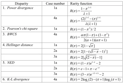
Table 1: Generation of diversities (rarity functions) from various disparities
Disparity Case number Rarity function
1. Power divergence 1a 1 1
( ) = 1 R
4a (2) 1 ( ) 1
( ) =
( 1) R
2. Pearson's chi-square 1a R( ) = (1 2) / 2
3. BWCS 4a (1 ) (1 2)
( ) =
2( 1)( 1)
R
4.Hellinger distance 1a R( ) = 2[1 ]
2a R( ) = 2[1 ( 1 1) ]2 3a R( ) = 2[ (2 ) 1]
5. NED 1a R( ) = (1 )e1 2
2a R( ) = e 1 e 3a R( ) = (3 )e (1 ) 2
Remark 2: Use of Case 1 and Case 2 (alternatively Case 3 and Case 4) may sometimes lead to the development of the same diversity (i.e., the same rarity function R) from the same disparity. For example, using the RAF A( ) = ( / 2)2 of the PCS in Case 1a and G function G( ) = 2/ 2 of PCS in Case 2a will result in the same rarity function
2 ( ) = (1 ) / 2
R . But this does not happen in general. For example, using the RAF
( ) = 2[ 1 1]
A of the HD in Case 1a we get the rarity function R( ) = 2[1 ], whereas use of the G function G( ) = 2[ 1 1]2 of the HD in Case 2a results in a different rarity function R( ) = 2[1 ( 1 1) ]2 . As a second example, one can see that use of the RAF A( ) = 2 (2 )e of the NED in Case 1a gives the rarity function R( ) = (1 )e1 2, whereas use of the G function ( ) = (G e 1 ) of the NED in Case 2a produces a different rarity function ( ) =R e 1 e.
5. Concluding remarks
Diversity measures have wide practical use for the measurement of ecological bio-diversity. In the traditional approach of measuring ecological diversity, one considers the relative abundances in a community without regard to the differences between species. For this scenario, the work by Patil and Taillie (1982) developed the appropriate concepts and provided a formal definition together with a logical framework. These authors defined diversity of a community as the average rarity of species within the community, and proposed a family of measures called diversity indices of degree .
The diversity measures defined under this approach are characterized by certain basic requirements. It turns out that a large and rich class of such measures satisfying these basic requirements may be constructed following the structure of the estimating functions in density-based minimum distance estimation. In this paper we demonstrate the construction of several such disparity measures based on different minimum distance procedures. The minimum disparity estimators considered here have show a great deal of variation in their behavior and we expect that the corresponding class of diversity measures will continue to show a responses leading to different interpretations.
Given the usefulness of measures of diversity, we expect that the link between the actual diversities and the class of minimum distance processes will act as a major facilitator in constructing useful diversity measures with the required properties. Clearly, more detailed studies and investigations will be required to select and choose the more suitable measures from within this class. But the availability of the class itself leads to useful gains, and represents the basis of important future selections.
References
2. Atkinson, A. B. (1970). On the measurement of inequality. Journal of Economic Theory, 2, 244-263.
3. Baczkowski, A. J., Joanes, D. N. and Shamia, G. M. (1997). Properties of a generalized diversity index. J. of Theoret. Biol., 188, 207.
4. Baczkowski, A. J., Joanes, D. N. and Shamia, G. M. (1998). Range of validity of
and for a generalized diversity index H( , ) due to Good. Mathematical Biosciences, 148, 115--128.
5. Baczkowski, A. J., Joanes, D. N. and Shamia, G. M. (2000). The distribution of a generalized diversity index due to Good. Environmental and Ecological Statistics, 7, 329--342.
6. Basu, A. and Lindsay, B. G. (1994). Minimum Disparity estimation in the continuous Case: Efficiency, Distributions, Robustness. Ann. Inst. Statist. Math., 46, 683--705.
7. Basu, A. and Sarkar, S. (1994). On disparity based goodness-of-fit tests for multinomial models. Statistics and Probability Letters19, 307-312.
8. Basu, A., Sarkar, S. and Vidyashankar, A. N. (1997). Minimum negative exponential disparity estimation in parametric models. J. Statist. Plann. Inf., 58, 349--370.
9. Basu, A., Shioya, H. and Park. C. (2011). Statistical Inference: The Minimum Distance Approach. Chapman & Hall/CRC, Boca Raton, Florida.
10. Beran, R. J. (1977). Minimum Hellinger distance estimates for parametric models. Ann. Statist., 5, 445--463.
11. Bhandari, S. K., Basu, A. & Sarkar, S. (2000). Robust estimation in parametric models using the family of generalized negative exponential disparities. Technical Report # 7/2000, Stat-Math Unit, Indian Statistical Institute, Calcutta 700108, India.
12. Champely, S. and Chessel, D. (2002). Measuring biological diversity using Euclidean metrics. Environmental and Ecological Statistics, 9, 167--177.
13. Cressie, N. and Read, T. R. C. (1984). Multinomial goodness-of-fit tests. J. Roy. Statist.Soc. B 46, 440-464.
14. Finkelstein, M.O. and Friedberg, R.M. (1967). The application of an entropy theory of concentration to the Clayton Act. Yale Law Journal, 76, 677-717. 15. Good, I. J. (1953). The population frequencies od species and the estimation of
population parameters. Biometrika, 40, 237--264.
16. Greenberg, J. H. (1956). The measurement of linguistic diversity. Language, 32, 109--115.
18. Jeong, D. and Sarkar, S. (2000). Negative exponential disparity based family of goodness-of-fit tests for multinomial models. J. Statist. Comput. Simul., 65, 43-61.
19. Lieberson, S. (1969). Measuring population diversity. American Sociological Review, 34, 850--862.
20. Light, R. J. and Margolin, B. H. (1971). An analysis of variance for categorical data. J. Amer. Stat. Assoc., 66, 534--544.
21. Lindsay, B. G. (1994). Efficiency versus robustness: the case for minimum Hellinger distance and related methods. Ann. Statist., 22, 1081--1114.
22. Nayak, T. K. (1986a). An analysis of diversity using Rao's quadratic entropy. Sankhya, Ser B, 48, 315--330.
23. Nayak, T. K. (1986b). Sampling distributions in analysis of diversity. Sankhya, Ser B, 48, 1--9.
24. Nei, R. K. (1973). The measurement of species diversity. Annual Review of Ecology and Systematics, 5, 285--307.
25. Patil, G. P. and Taillie, C. (1982). Diversity as a concept and its measurement. J. Amer. Statist. Assoc., 77, 548--567.
26. Rao, C. R. (1982a). Diversity: its measurement, decomposition, apportionment and analysis. Sankhya, Ser A, 44, 1--21.
27. Rao, C. R. (1982b). Diversity and dissimilarity coefficients: a unified approach. Theoretical Population Biology, 21, 24--43.
28. Sen, A. (1974). Poverty, inequality and unemployment: some conceptual issues issues in measurement. Sankhya, Ser. C 36, 67--82.
29. Shannon, C. E.(1948). A mathematical theory of communication. Bell System Tech. J., 27, 379.
30. Shin, D. W., Basu, A. and Sarkar, S (1995). Comparison of the blended weight Hellinger distance based goodness-of-fit test statistics. Sankhya, Ser. B 57, 365-376.
31. Shin, D. W., Basu, A. and Sarkar, S (1996). Small sample comparison for the blended weight chi-square goodness-of-fit test statistics. Commun. Statist. Theory Meth., 25, 211-226.
32. Simpson, D. G. (1987). Minimum Hellinger distance estimation for analysis of count data. J. Amer. Statist. Assoc., 82, 802--807.
33. Simpson, D. G. (1989). Hellinger deviance tests: Efficiency, breakdown points and examples. J. Amer. Statist. Assoc., 84, 107--113.
34. Simpson, E. H.(1949). Measurement of diversity. Nature, 163, 688.
36. Tamura, R. N. and Boos, D. D. (1986). Minimum Hellinger distance estimation for multivariate location and covariance. J. Amer. Statist. Assoc., 81, 223--229. 37. Tomizawa, S. (1994). Two kinds of measures of departure from symmetry in
square contingency tables. Statistica Sinica, 4, 548--561.
38. Tomizawa, S., Seo, T. and Ebi, M. (1997). Generalized proportional reduction in variation measure for two-way contingency tables. Behaviormetrika, 24, 193--201.
39. Tomizawa, S., and Ebi, M. (1998). Generalized proportional reduction in variation measure for multi-way contingency tables. Journal of Statistical Research, 32, 75--84.