Poisson Distribution under various Loss Functions
Sanku Dey
Department of Statistics St. Anthony’s College Shillong, Meghalaya India
Tanujit Dey
Department of Mathematics The College of William & Mary Williamsburg, Virginia, USA. [email protected]
Abstract
The performance of Bayes estimators depend on the form of the prior distribution and the assumed loss function. This paper resolves the problem of estimation of one parameter decapitated generalized Poisson distribution; using a class of improper prior distributions under symmetric and asymmetric loss functions. The statistical performances of the Bayes estimates with respect to different priors and loss functions are illustrated for a data set and a simulation study.
Keywords: Bayes estimator, Decapitated generalized Poisson distribution, General entropy loss function, Quadratic loss function, Squared error loss function.
1. Introduction
Discrete distributions are finding their way into Bayesian analysis. The literature dealing with discrete distributions is sparse as far as Bayesian inference is concerned. For a bibliography of relevant literature, see Hassan et al (2007a, 2007b), Hassan and Khan (2009). Considering a random variable X that follows a decapitated generalized Poisson distribution (DGPD) with one parameter
when the other parameter is assumed to be known, the probability function of X is given by1
(1 ) (1 ) 1 1
( ) (1 ) ; 1, 2, ...; 0, 0 .
! x
x x x
P X x e e x
x
(1)
This paper sites Bayes estimators of decapitated generalized Poisson distribution (DGPD) for one parameter, when the other parameter is assumed to be known under different loss functions.
2. Bayes Estimation
In this section, we estimate the unknown parameter of the DGPD based on a sample of size n from (1). The likelihood function of the random sample x = (x1, x2, . . . , xn) is given by
(
)
( |
)
y
n
y
(1
)
n
L x
K
e
e
(2)1
(1 )
where [ ] and .
! 1
1
x
n i n
xi
K y xi
x i
i i
2.1. Prior Distribution
The Bayesian formulation requires appropriate prior(s) for the parameter(s). If we have enough information that can help us to go for an informative prior, it would certainly be preferred over all other choices. Otherwise it is better to stick to non-informative or vague priors. In this paper, we have considered the following prior (See Upadhyay et al. (2001), Singpurwalla (2006)).
1
( ) ; 0
g c
c
(3)
Here c = 0 leads to a diffuse prior and c = 1 to a non-informative prior.
2.2. Loss Function
From a theoretical decision perspective, in order to select the 'best' estimator, a loss function must be specified and the loss function is used to represent a penalty associated with each of the possible estimates. Traditionally, most authors use the simple squared error loss function to obtain the posterior mean as the Bayesian estimate. However, in practice, the real loss function is often not symmetric. In recent years, many authors have considered asymmetric loss functions. Here we consider symmetric as well as asymmetric loss functions for our Bayesian analysis.
1. The first loss function considered is a quadratic loss function and is given by
1
1
- 2 ( , ) ( ) 1
L
2. The second loss function considered is the General entropy loss function. In many practical situations; it appears to be more realistic to express the loss, in terms of ratio (
/ ). Calabria and Pulcini (1996) proposed a loss function called General Entropy Loss Function of the form:2 2
( ,
)
(
)
log(
) 1
;
0;
0,
2
2
p
L
w
p
w
p
(4)where the minimum occurs when 2 .
This loss is a generalization of the Entropy loss, referred to by several authors (see, Dey et al (1987) and Dey and Liu (1992)), where the shape parameter p is equal to 1.The Bayes estimator for the parameter (when w = 1) under General Entropy loss may be defined as
1
( p) p E
provided that E(
p) exists, and is finite. The proper choice for p is a challenging problem for analyst as it reflects the asymmetry of the loss function in a given practical situation. A discussion towards finding a solution for such type of problem is available in Calabria and Pulcini (1996).3. The third loss function is the squared log error loss function proposed by Brown (1968), and is defined as
(5)
which is balanced and lim ( , ) 0 .
3 3 3
L as or This loss is not always
convex, it is convex for 3 e
and concave else wise, but its risk function has a
unique minimum with respect to 3
.
The posterior expectation of (5) is
2
3 3 3 3
2
( , )| log( ) 2 log( ) log( )| (log( )) | . E L y E y E y (6)
Under the squared log error loss function, the Bayes estimator for parameter of DGPD is the value which minimizes (6). It is
ˆ exp[ (log( ) | )]E y
provided that E(log( ) | ) y exists, and is finite.
2 3 23
( ,
3)
log
3log
log(
)
L
2.3. Posterior Distribution
Combining the prior distribution (3) and the likelihood function (2), the posterior distribution of is derived as
( )
( )
0
(1
)
(
| )
;
0.
(1
)
y c n y n
y c n y n
e
e
y
e
e
d
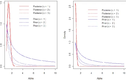
(7)From Figure (1), the posterior of appear to be quite robust irrespective of variations in c. It’s worth noting that the prior (3) is not exactly non-informative; with changes in c, the priors show significant change. Looking at the corresponding posteriors, there is not enough changes in the shape and the robustness of the densities, even though the sample is small (n = 10), but the robustness is quite noticeable for the plot with sample size n = 30.
Figure 1: Plots to represent the interplay between the prior (3) and the posterior density (7) for . The left plot is put together using fixed value for n = 10,
1 / 3
and y = 37, whereas for the right plot, the fixed value for n = 30, 1 / 3
2.4. Bayes estimator under quadratic loss function (BEQF)
Under prior (3), The Bayes estimator for the parameter with the posterior density (7) is given by
1 ( ) 0
1
2 ( ) 0
(1
)
.
(1
)
y c n y n
y c n y n
e
e
d
e
e
d
After simplification, we get
1
( ) 1
( )
0
ˆ .
( 1) 1
1
( )
0
y c n k C
k y c
n y k
k
y c n k C
k y c
n y k
k
(8)
2.5. Bayes estimator under general entropy loss function (GELF)
Under prior (3), The Bayes estimator for the parameter with the posterior density (7) is given by
1
2
0
1
ˆ
(
)
(
|
)
.
p p
p
p
E
y d
After simplification, we get
1
( 1)
1
1
( )
0
2 ( 1)
1
1
( )
0
ˆ
.
y p c p
n k
Ck n y k y p c
k
y c n k
Ck n y k y c
k
(9)Remark
When p= 1, the Bayes estimator (9) coincides with the Bayes estimator
under the weighted squared error loss function of the form
2 ( )
.
2.6. Bayes estimator under squared log error loss function(BESLF)
Under the above prior (3) and posterior distribution (7) and using the squared log error loss function, the Bayes estimator for parameter of DGPD is the value which minimizes (6). It is computed as
3
0
ˆ
exp
E
(log( ) |
y
)
exp[
log( ) (
|
y d
)
.
After algebraic manipulation,
1 1
0
1
1 0
1
( ) ( 1)[ ( 1) log( )]
(log( ) | )
( 1)
( )
n k y c
k k
n k
k y c
k
C y c y c n y k
n y k
E y
y c C
n y k
Where
(y c 1) d log (y c 1) is the digamma function.
dy
Hence, we have,
1 1
0 3
1
1 0
1
( ) ( 1)[ ( 1) log( )]
ˆ exp .
( 1)
( )
n k y c
k k
n k
k y c
k
C y c y c n y k
n y k
y c C
n y k
(10)3. Simulation and Discussion
This section conducts a Monte Carlo simulation study to compare the performance of the different Bayes estimators. The mean square error (MSE) is used to compare the estimates. For this simulation study, we have chosen
n = 10, 20, 30, 40. Tables 3- 6 summarizes the results of the simulation study for different values of α =1, 2 ; β=1/3, 1/2, 1/6 and 1/8; w = 1; c = 1, 2, 3 and
1, 2, 3
p . The estimators are computed along with their MSE. Tables 3 and 4 present results for α = 1 and β = 1/3 and 1/2. Tables 5 and 6 present results for α = 2 and β = 1/6 and 1/8. We summarize the results as follows.
1. Tables 3 - 6, illustrate that our prior underestimates the true value of the parameter under all loss functions irrespective of the value of c, but under the entropy loss function, with negative values of p, present values
nearer to the true value of the parameter. We also observe that for any
values of p gives the smallest MSE's than the corresponding MSE's from
the other two loss functions. A detailed and thorough study of the simulated MSE reveals that the three Bayes estimators show slight change in the value of their MSE's for the variation of c when sample size increases.
2. In the case of general entropy loss, MSE's remains more or less the same with positive or negative values of the constant value of p when sample
size n > 30. However estimates show a profound change with variation in c. Also MSE decreases when the values increases and vice-versa.
3. On the basis of the above observation, we conclude that the MSE's of Bayes estimators are not responsive to the choices of the parameter c when n 30. Finally, the Bayes estimator using the General entropy loss function could be effectively employed, instead of Bayes estimators using a quadratic loss and squared log error loss functions with a proper choice of p.
4. Application and Conclusion
In this section we compare the several proposed estimation techniques based on a data set. Assuming that only the counts are given, rather than the ordered raw data, we fit the decapitated generalized Poisson distribution to the data via Bayesian methods.
Table 1: Abortion data
Number of cases 1 2 3 4 6 7
Frequency 7 7 3 3 1 2
The data set given in Table 1 consists of frequency of trisomy among karyotyped spontaneous abortions of pregnancies, by calendar month of the last menstrual period, for the period of July 1975 to June 1977, in three New York hospitals. For details of the data, see Wallenstein (1980). To calculate Bayesian estimators, we have used several values of and c for this data set, we notice that the = 1/8 and c = 1 provide reasonable fit to the data set. In Table 2 we see that the fitted probabilities corresponding to three different estimators effectively echo the same trend of inference as seen in the simulation study.
Acknowledgment
Table 2: Empirical and fitted probability distributions for abortion data
Cases Observed Fitted
1
2
2
2
31
p p 1 p2 p 2 p3 p 3
1 0.3043 0.3177 0.3083 0.2991 0.3130 0.2947 0.3178 0.2903 0.3036 2 0.3043 0.2673 0.2643 0.2611 0.2658 0.2595 0.2673 0.2579 0.2627 3 0.1304 0.1814 0.1828 0.1839 0.1821 0.1844 0.1814 0.1848 0.1834 4 0.1304 0.1090 0.1119 0.1146 0.1105 0.1160 0.1090 0.1172 0.1133 6 0.0435 0.0320 0.0341 0.0363 0.0331 0.0373 0.0320 0.0384 0.0352 7 0.0870 0.0163 0.0177 0.0192 0.0170 0.0199 0.0163 0.0206 0.0184
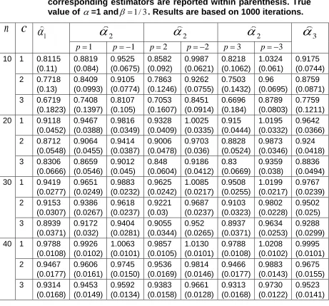
Table 3: Three different estimators for the parameter with values of
c = 1; 2; 3; n = 10; 20; 30; 40 and p = 1; 2; 3. MSE of the corresponding estimators are reported within parenthesis. True value of =1 and 1 / 3. Results are based on 1000 iterations.
n
c
1
2
2
2
31
p p 1 p2 p 2 p3 p 3
10 1 0.8115 (0.11) 0.8819 (0.084) 0.9525 (0.0675) 0.8582 (0.092) 0.9987 (0.0621) 0.8218 (0.1062) 1.0324 (0.061) 0.9175 (0.0744) 2 0.7718
(0.13) 0.8409 (0.0993) 0.9105 (0.0774) 0.7863 (0.1246) 0.9262 (0.0755) 0.7503 (0.1432) 0.96 (0.0695) 0.8759 (0.0871) 3 0.6719
(0.1823) 0.7408 (0.1397) 0.8107 (0.105) 0.7053 (0.1607) 0.8451 (0.0914) 0.6696 (0.184) 0.8789 (0.0803) 0.7759 (0.1211) 20 1 0.9118
(0.0452) 0.9467 (0.0388) 0.9816 (0.0349) 0.9328 (0.0409) 1.0025 (0.0335) 0.915 (0.0444) 1.0195 (0.0332) 0.9642 (0.0366) 2 0.8712
(0.0548) 0.9064 (0.0455) 0.9414 (0.0387) 0.9006 (0.0478) 0.9703 (0.036) 0.8828 (0.0524) 0.9873 (0.0346) 0.924 (0.0418) 3 0.8306
(0.0666) 0.8659 (0.0546) 0.9012 (0.045) 0.848 (0.0604) 0.9186 (0.0412) 0.83 (0.0669) 0.9359 (0.038) 0.8836 (0.0494) 30 1 0.9419
(0.0277) 0.9651 (0.0249) 0.9883 (0.0232) 0.9625 (0.0242) 1.0085 (0.0217) 0.9508 (0.0255) 1.0199 (0.0217) 0.9767 (0.0239) 2 0.9153
(0.0307) 0.9386 (0.0267) 0.9618 (0.0237) 0.9221 (0.03) 0.9687 (0.0237) 0.9103 (0.0323) 0.9802 (0.0228) 0.9502 (0.025) 3 0.8939
(0.0371) 0.9172 (0.032) 0.9404 (0.0281) 0.9055 (0.0344) 0.952 (0.0265) 0.8937 (0.0371) 0.9634 (0.0253) 0.9288 (0.0299) 40 1 0.9788
(0.0108) 0.9926 (0.0102) 1.0063 (0.0101) 0.9857 (0.0105) 1.0130 (0.0101) 0.9788 (0.0108) 1.0208 (0.0102) 0.9995 (0.0101) 2 0.9467
(0.0177) 0.9606 (0.0161) 0.9745 (0.0150) 0.9536 (0.0169) 0.9814 (0.0146) 0.9466 (0.0177) 0.9883 (0.0143) 0.9675 (0.0155) 3 0.9314
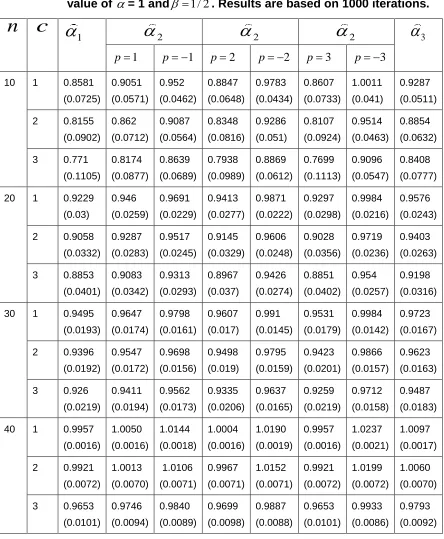
Table 4: Three different estimators for the parameter with values of
c = 1; 2; 3; n = 10; 20; 30; 40 and p = 1; 2; 3. MSE of the corresponding estimators are reported within parenthesis. True value of = 1 and 1/ 2. Results are based on 1000 iterations.
n
c
1
2
2
2
31
p p 1 p2 p 2 p3 p 3
10 1 0.8581 (0.0725) 0.9051 (0.0571) 0.952 (0.0462) 0.8847 (0.0648) 0.9783 (0.0434) 0.8607 (0.0733) 1.0011 (0.041) 0.9287 (0.0511)
2 0.8155 (0.0902) 0.862 (0.0712) 0.9087 (0.0564) 0.8348 (0.0816) 0.9286 (0.051) 0.8107 (0.0924) 0.9514 (0.0463) 0.8854 (0.0632)
3 0.771 (0.1105) 0.8174 (0.0877) 0.8639 (0.0689) 0.7938 (0.0989) 0.8869 (0.0612) 0.7699 (0.1113) 0.9096 (0.0547) 0.8408 (0.0777)
20 1 0.9229 (0.03) 0.946 (0.0259) 0.9691 (0.0229) 0.9413 (0.0277) 0.9871 (0.0222) 0.9297 (0.0298) 0.9984 (0.0216) 0.9576 (0.0243)
2 0.9058 (0.0332) 0.9287 (0.0283) 0.9517 (0.0245) 0.9145 (0.0329) 0.9606 (0.0248) 0.9028 (0.0356) 0.9719 (0.0236) 0.9403 (0.0263)
3 0.8853 (0.0401) 0.9083 (0.0342) 0.9313 (0.0293) 0.8967 (0.037) 0.9426 (0.0274) 0.8851 (0.0402) 0.954 (0.0257) 0.9198 (0.0316)
30 1 0.9495 (0.0193) 0.9647 (0.0174) 0.9798 (0.0161) 0.9607 (0.017) 0.991 (0.0145) 0.9531 (0.0179) 0.9984 (0.0142) 0.9723 (0.0167)
2 0.9396 (0.0192) 0.9547 (0.0172) 0.9698 (0.0156) 0.9498 (0.019) 0.9795 (0.0159) 0.9423 (0.0201) 0.9866 (0.0157) 0.9623 (0.0163)
3 0.926 (0.0219) 0.9411 (0.0194) 0.9562 (0.0173) 0.9335 (0.0206) 0.9637 (0.0165) 0.9259 (0.0219) 0.9712 (0.0158) 0.9487 (0.0183)
40 1 0.9957 (0.0016) 1.0050 (0.0016) 1.0144 (0.0018) 1.0004 (0.0016) 1.0190 (0.0019) 0.9957 (0.0016) 1.0237 (0.0021) 1.0097 (0.0017)
2 0.9921 (0.0072) 1.0013 (0.0070) 1.0106 (0.0071) 0.9967 (0.0071) 1.0152 (0.0071) 0.9921 (0.0072) 1.0199 (0.0072) 1.0060 (0.0070)
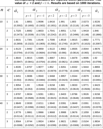
Table 5: Three different estimators for the parameter with values of c = 1; 2; 3; n = 10; 20; 30; 40 and p = 1; 2; 3. MSE of the corresponding estimators are reported within parenthesis. True value of = 2 and 1/ 6. Results are based on 1000 iterations.
n
c
1
2
2
2
31
p p 1 p2 p 2 p3 p 3
10 1 1.81 (0.2002) 1.8851 (0.1693) 1.9596 (0.1502) 1.8416 (0.1931) 1.991 (0.1519) 1.803 (0.2116) 2.0273 (0.149) 1.9226 (0.1582)
2 1.7325 (0.2473) 1.8082 (0.2039) 1.8833 (0.1725) 1.7541 (0.2242) 1.9051 (0.157) 1.715 (0.2496) 1.9418 (0.148) 1.846 (0.1866)
3 1.6631 (0.2859) 1.7391 (0.2322) 1.8146 (0.1905) 1.7006 (0.2581) 1.8516 (0.1745) 1.6615 (0.2877) 1.8882 (0.1615) 1.7771 (0.2097)
20 1 1.9123 (0.0794) 1.9492 (0.0725) 1.9859 (0.0684) 1.9122 (0.0768) 1.9862 (0.066) 1.8935 (0.0814) 2.0044 (0.065) 1.9676 (0.0701)
2 1.8643 (0.0947) 1.9015 (0.0841) 1.9385 (0.0764) 1.8667 (0.1004) 1.9411 (0.0821) 1.8478 (0.1069) 1.9595 (0.0794) 1.92 (0.0799)
3 1.8335 (0.1047) 1.8707 (0.0918) 1.9077 (0.0817) 1.852 (0.0979) 1.9261 (0.0778) 1.8332 (0.1049) 1.9444 (0.0746) 1.8893 (0.0864)
30 1 1.9451 (0.053) 1.9696 (0.0501) 1.9940 (0.0484) 1.9468 (0.0465) 1.9957 (0.0423) 1.9344 (0.0483) 2.0079 (0.042) 1.9818 (0.0491)
2 1.9054 (0.0578) 1.93 (0.053) 1.9546 (0.0494) 1.9158 (0.0592) 1.965 (0.0517) 1.9033 (0.0619) 1.9771 (0.0506) 1.9423 (0.051)
3 1.8787 (0.0648) 1.9034 (0.0586) 1.9281 (0.0536) 1.8911 (0.0615) 1.9403 (0.0516) 1.8786 (0.0648) 1.9526 (0.0499) 1.9158 (0.0559)
40 1 1.9849 (0.0437) 2.0030 (0.0396) 2.0211 (0.0362) 1.9940 (0.0416) 2.0391 (0.0348) 1.9849 (0.0437) 2.0391 (0.0335) 2.0121 (0.0378)
2 1.9776 (0.0114) 1.9861 (0.0111) 1.9966 (0.0114) 1.9668 (0.0112) 1.9988 (0.0118) 1.9676 (0.0114) 2.1059 (0.0123) 1.9954 (0.0111)
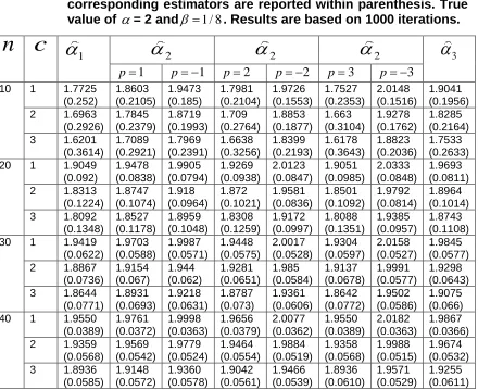
Table 6: Three different estimators for the parameter with values of c = 1; 2; 3; n = 10; 20; 30; 40 and p = 1; 2; 3. MSE of the corresponding estimators are reported within parenthesis. True value of = 2 and 1 / 8. Results are based on 1000 iterations.
n
c
1
2
2
2
31
p p 1 p2 p 2 p3 p 3
10 1 1.7725 (0.252) 1.8603 (0.2105) 1.9473 (0.185) 1.7981 (0.2104) 1.9726 (0.1553) 1.7527 (0.2353) 2.0148 (0.1516) 1.9041 (0.1956) 2 1.6963
(0.2926) 1.7845 (0.2379) 1.8719 (0.1993) 1.709 (0.2764) 1.8853 (0.1877) 1.663 (0.3104) 1.9278 (0.1762) 1.8285 (0.2164) 3 1.6201
(0.3614) 1.7089 (0.2921) 1.7969 (0.2391) 1.6638 (0.3256) 1.8399 (0.2193) 1.6178 (0.3643) 1.8823 (0.2036) 1.7533 (0.2633) 20 1 1.9049
(0.092) 1.9478 (0.0838) 1.9905 (0.0794) 1.9269 (0.0938) 2.0123 (0.0847) 1.9051 (0.0985) 2.0333 (0.0848) 1.9693 (0.0811) 2 1.8313
(0.1224) 1.8747 (0.1074) 1.918 (0.0964) 1.872 (0.1021) 1.9581 (0.0836) 1.8501 (0.1092) 1.9792 (0.0814) 1.8964 (0.1014) 3 1.8092
(0.1348) 1.8527 (0.1178) 1.8959 (0.1048) 1.8308 (0.1259) 1.9172 (0.0997) 1.8088 (0.1351) 1.9385 (0.0957) 1.8743 (0.1108) 30 1 1.9419
(0.0622) 1.9703 (0.0588) 1.9987 (0.0571) 1.9448 (0.0575) 2.0017 (0.0528) 1.9304 (0.0597) 2.0158 (0.0527) 1.9845 (0.0577) 2 1.8867
(0.0736) 1.9154 (0.067) 1.944 (0.062) 1.9281 (0.0651) 1.985 (0.0584) 1.9137 (0.0678) 1.9991 (0.0577) 1.9298 (0.0643) 3 1.8644
(0.0771) 1.8931 (0.0693) 1.9218 (0.0631) 1.8787 (0.073) 1.9361 (0.0606) 1.8642 (0.0772) 1.9502 (0.0586) 1.9075 (0.066) 40 1 1.9550
(0.0389) 1.9761 (0.0372) 1.9998 (0.0363) 1.9656 (0.0379) 2.0077 (0.0362) 1.9550 (0.0389) 2.0182 (0.0363) 1.9867 (0.0366) 2 1.9359
(0.0568) 1.9569 (0.0542) 1.9779 (0.0524) 1.9464 (0.0554) 1.9884 (0.0519) 1.9358 (0.0568) 1.9988 (0.0515) 1.9674 (0.0532) 3 1.8936
(0.0585) 1.9148 (0.0572) 1.9360 (0.0578) 1.9042 (0.0561) 1.9466 (0.0539) 1.8936 (0.0610) 1.9571 (0.0529) 1.9255 (0.0611) References
1 Brown, L.D. (1968). Inadmissibility of the usual estimators of scale parameters in problems with unknown location and scale parameters. Ann. Math. Statist. 39, 29 - 48.
2. Calabria, R. and Pulcini, G. (1996). Point estimation under asymmetric loss functions for left truncated exponential samples. Commun. Statist - Theory Meth., 25(3), 585-600.
3. Consul, P.C. (1989). Generalized Poisson distribution, Properties and applications, John Wiley, New York.
4. Consul, P.C. and Famoye, F. (1989). The truncated generalized Poisson distribution and its applications, Commun. Statist - Theory Meth., 18(10), 3635 - 3648.
6. David, F.N. and Johnson, N.L. (1952). The truncated Poisson, Biometrics, 8, 275-285.
7. Dey, D.K., Ghosh, M. and Srinivasan, C. (1987). Simultaneous estimation of parameters under entropy loss. J. Statist. Plann. Inference, 15, 347-363.
8. Dey, D.K. and Liu, P. L. (1992). On comparison of estimators in a generalized life model. Microelectron. Reliab., 32, 207-221.
9. Hassan, A., Mir, K. A., and Ahmad, M. (2007a). Bayesian analysis and reliability function of decapitated generalized Poisson distribution. Pak. J. of Statist. 23(3), 221-230.
10. Hassan, A., Mir, K. A., and Ahmad, M. (2007b). On Bayesian analysis of generalized geometric series distribution under different priors. Pak. J. of Statist. 23(3), 221-230.
11. Hassan, A. and Khan, S. (2009). Prediction distribution of generalized geometric series distribution and its different forms. Pak. J. of Statist. 25(1), 47-57.
12. Jani, P.N. and Shah, S.M. (1981). The truncated generalized Poisson distribution. Aligarh Journal of Statistics, 1(2), 174-182.
13. Johnson, N.L, Kotz, S. and Kemp. A.W. (1992). Univariate discrete distribution, John Willy and Sons, New York.
14. Singpurwalla, N.D. (2006). Reliability and Risk: A Bayesian Perspective. Wiley, New York.
15. Upadhyay, S.K., Vasistha, N. and Smith, A.F.M. (2001). Bayes inference in life testing and reliability via Markov chain Monte Carlo simulation, Sankhya A, 63, 15-40.