A Comparative Study on the Performance of New Ridge Estimators

(1)

A Comparative Study on the Performance of New Ridge Estimators

Satish Bhat

Department of Statistics, Yuvaraja’s College

University of Mysore, Mysore, Karnataka, India-570005 [email protected]

Vidya, R.

Department of Statistics, Yuvaraja’s College

University of Mysore, Mysore, Karnataka, India-570005 [email protected]

Abstract

Least square estimators in multiple linear regressions under multicollinearity become unstable as they produce large variance for the estimated regression coefficients. Hoerl and Kennard 1970, developed ridge estimators for cases of high degree of collinearity. In ridge estimation, the estimation of ridge parameter (k) is vital. In this article new methods for estimating ridge parameter are introduced. The performance of the proposed estimators is investigated through mean square errors (MSE). Monte-Carlo simulation technique indicated that the proposed estimators perform better than ordinary least squares (OLS) estimators as well as few other ridge estimators.

Keywords: Multiple Linear Regression, Multicollinearity, Ridge Parameter and MSE.

1. Introduction

Consider the classical linear regression model u

β X

y= + , (1)

where X is a (n× ) matrix of non-stochastic regressors, p β is a (p×1) vector of the unknown regression coefficients and u be a (n×1) vector of random disturbances such that E[u]=0and E[uu′]=σ2I. For computational point of view X is normalized and y is expressed in deviations from mean. Ordinary least squares give the estimator forβ as



XX



Xy

OLS   

1

ˆ

 provided



XX



-1exist. OLS is an unbiased estimator. But when multicollinearity is present in the data, OLS estimator becomes unstable due to their large variance, which may lead to poor prediction. To overcome this condition, the most popular and commonly used estimator is the ridge estimator and it was first introduced by Hoerl and Kennard 1970. They defined the ordinary ridge estimator as





OLS

R XX kI XX

ˆ _ _ _ -1 _ ˆ

(2)

Motivation for this paper is to study the performance of ridge estimators available in the literature and to suggest modified estimators when multicollinearity is present in the data. This article is restricted to deal multicollinearity problem. The proposed modified estimators are evaluated using Monte-Carlo simulation and compared in terms of ratio of average MSE (AMSE) of OLS over other existing ridge estimators.

For computational ease and for further discussion we express equation (1) in canonical form as

, + =Zγ u

y (2)

where Z=XW,γ=W′β andZ′Z =W′X′XW =D=diag(λ1,λ2,...,λp), where Wbe a (p×p) matrix such that its columns are normalized eigen vectors ofX′, X λ_i' are the s

th

j eigen value ofX′X . The ordinary least squares (OLS) estimator of y is then given by

 

.

ˆ 1 1

y Z D y Z Z Z

OLS     

 

 (3)

Since γ=W′β, implies βˆ =Wγˆ. 2. Ordinary Ridge Estimator

By adding a biasing constant k to the th

i element of the diagonal of the matrix Z′Z (defined as in (3)), the ordinary ridge estimator (ORR) of γcan be written as





,

ˆ 1 1

y Z A y Z kI D

R     

 

 (4)

whereA DkI. From equations (3) and (4), we write





ˆ ,

ˆ ₁ 1

OLS

R I A k 

 _ _  

(5)

The bias of γˆ is given by _R . )

ˆ

( A 1k

bias _R   (6)

Therefore the bias of βˆ is

. )

ˆ ( )

ˆ

(  1 

W kWA bias

W

bias  _R    (7)

The mean square error of γˆ is given by _R

. ) + ( + ) + ( ˆ =

) ˆ ( ]′ ) ˆ ( [ + ) ˆ ( var = ) ˆ (

∑

1

= =1

2 2 2

2 2

p

i

p

i i

i

i i

R R

k λ

γ k

k λ

λ σ

γ bias γ

bias γ

iance γ

MSE

(8)

3. Proposed Estimators

(3)

, ˆ ≤ ≤ 0 ₂ max 2 γ σ

k the MSE(γˆ_R)is minimum, where 2 max

γ is the largest element of γ2and _σ2

is replaced by its estimate

1 ˆ ˆ2       p n y Z y

y _OLS

 . In the case of ORR, various methods for estimating the ridge parameter (k) were defined and some of the well known methods are listed below:

i) γ γ σ p k_HKB ˆ ′ ˆ ˆ = 2

(Hoerl, Kennard and Baldwin 1975) (11)

ii)

∑

1 = 2 2 ˆ ˆ = _p i i i LW γ λ σ p

k (Lawless and Wang 1976) (12)

iii)

(

)

[

]

{

}

∑

1 = 2 / 1 2 2 2 2 ] ˆ / ˆ [ + 1 + 1 / ˆ ˆ = _p i i i i HMO σ γ λ γ σ p

k , (Nomura 1988) (13)

iv)



₂



max max 2 2 max ˆ ˆ ) 1 ( ˆ          p n

k_KS , (Khalaf and Shukur 2005) (14)

where λmax is the largest eigen value ofX′X.

v) _

         max 2 ) ( 1 ˆ ˆ ˆ , 0 j DK VIF n p Max k   

, (Dorugade and Khashid 2010) (15)

where , 1,2,..., ; 1

1

2 j p

R VIF

j

j  _  is the variance inflation factor of the th j regressor. vi)

∑

1 = 2 2 max ˆ ˆ 2 = ) ( p i i AD _γ σ λ Mean Harmonic

k (Dorugade 2014) (16)

The estimator HKB still works better in terms of MSE. The estimators DK and AD

proposed by Dorugade and Khashid 2010 and Dorugade 2014 respectively, perform better than HKB when there exist a very high degree (ρ≥0.9) of collinearity among the predictors, which may not be realistic in real life situations. Simulation study indicates that when there is low or moderate or high degree of collinearity, the estimators KS,

HMO and LW may tend to be unstable for the lower error variance. To overcome these we propose two modified estimators for determining ridge parameterk,and following Hoerl et al. 1975, the suggested modified estimators are defined as:

vii) γ γ λ k γ γ λ γ γ σ p

k_SV _HKB

ˆ ′ ˆ 1 + = ˆ ′ ˆ 1 + ˆ ′ ˆ ˆ = max max 2

(4)

viii)

m k

λ λ γ

γ σ p

k_SV _HKB

2 1 + =

) / ( 2

1 +

ˆ ′ ˆ

ˆ

= ₂

min max 2

2 (18)

where m= λmax /λmin is called the condition number (Weisberg-1985, Chatterjee and

Hadi-1988. Higher the value ofm, higher is the degree of multicollinearity. If m is between 30-100 indicates moderate to strong correlation and if m is more than 100 suggests severe multicollinearity (Liu 2003). The simulation study indicate that suggested estimators defined as in (17) and (18) respectively perform better when data is suffering from low, moderate and high degree of collinearity. The suggested estimators SV1 and

SV2 take little over bias than Hoerl and Kennard 1970 but they minimise the total

variance.

4. The Results of Simulation Study

The performance of the estimators is studied through Monte-Carlo simulation. The performance of these estimators is investigated in the presence of low, moderate and high degree of multicollinearity. The results are obtained by generating a random matrix X of size (n× ) using the relation p _x (1 2)1/2 ,_i 1,2,...,_n;_j 1,2,...,_p;

ip ij

ij       where

ij

ξ is an independent standard normal pseudo-random number, ρis specified such that

2

ρ is the degree of correlation between any two predictors. These predictor variables are standardized such that XX′is in the correlation form and it is used to generate ywith

]′ 4 . 0 , 5 . 0 , 9 . 0 , 3 . 0 , 5 . 0 , 3 . 0 [ =

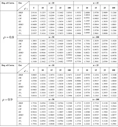
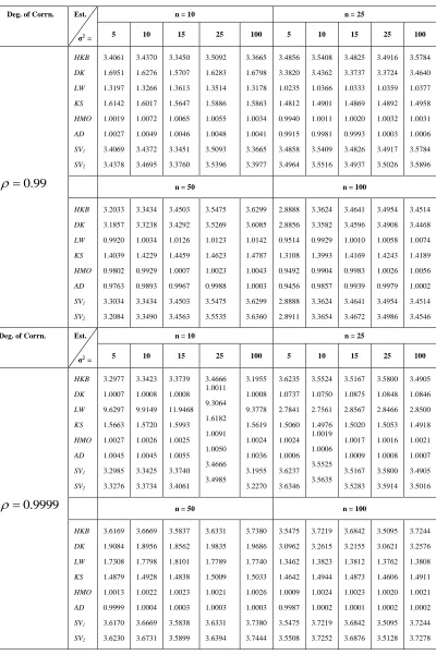
β . To study the performance of the proposed estimators we have assumed various values for n as 10, 25, 50 and 100; variances of the residual term as 5, 10, 15, 25 and 100 and the degree of correlation ρas 0.8, 0.9, 0.99 and 0.9999. Experiment is repeated 5000 times each and average mean square error (AMSE) is computed. Ridge estimates are computed by considering the different estimators of the ridge parameter (k) defined as in equations (11) to (18). Here we consider the process that leads to the maximum ratio of AMSE of OLS over AMSE of other ridge estimators to be the best in terms of MSE point of view. From tables - I and II, we observe that the performance of the suggested ridge estimators is better and comparable than the other estimators in almost all cases. However when there is a wide range of moderate or high degree of collinearity the estimator

2

SV

k performs considerably better than all other estimators considered under study. If we observe carefully, the suggested estimators and as well the other estimators may vary little (under estimates on comparing with OLS) when the sample size (n) is large, degree of correlation is less and variance σ2of the error terms are small (Ref. table - 1 for n =100; and error variance _σ2

= 5 and ρ= 0.8). We observe the performance of different estimators from the Figures 1and 2. Figure 1 is drawn for AMSE ratio against various values of sample size n, whenρand _σ2

are fixed and Figure 2 is drawn for AMSE ratio against various values of error variance _σ2

(5)

performance of the estimators LW, AD, HMO, and KS are similar hence forming two groups in terms of their performance. A through study has to be done in this regard. 5. Conclusion

The ridge estimators studied in this article are computed for varied combinations of sample sizes (n), variance (σ2) of the error term and degree of correlation (ρ) between the predictors. The suggested estimators are evaluated and compared with other ridge estimators. Experiment is repeated 5000 times each and average mean square errors (AMSEs) are computed. When there is wide range of degree of collinearity among the predictors the performance of the suggested estimators is satisfactory and slightly better over other ridge estimators considered in this articles.

Table 1: AMSE ratio of OLS estimator over different Ridge estimators

Deg. of Corrn. Est.

σ2 ₌

n = 10 n = 25

5 10 15 25 100 5 10 15 25 100

8 . 0   HKB DK LW KS HMO AD SV1 SV2 2.9116 2.6919 0.9869 1.4479 0.9688 0.9664 2.9123 2.9397 3.1253 2.8562 1.0313 1.5122 1.0078 0.9997 3.1255 3.1616 3.2248 3.0299 1.0283 1.5336 1.0069 1.0014 3.2249 3.2606 3.3462 3.1404 1.0315 1.5634 1.0108 1.0046 3.3462 3.3833 3.0541 2.8113 1.0258 1.5057 1.0100 1.0038 3.0541 3.0896 1.9352 1.9319 0.8327 1.0358 0.8349 0.8314 1.9353 1.9406 2.6886 2.6824 0.9591 1.2387 0.9633 0.9576 2.6886 2.6985 2.9750 2.9683 0.9803 1.2879 0.9844 0.9786 2.9750 2.9861 2.9889 2.9815 0.9945 1.3019 0.9991 0.9929 2.9889 3.0008 3.1266 3.1192 1.0017 1.3222 1.0061 1.0005 3.1266 3.1391

n = 50 n = 100

HKB DK LW KS HMO AD SV1 SV2 1.3093 1.3089 0.6826 0.7747 0.6856 0.6823 1.3093 1.3108 2.3401 2.3392 0.8990 1.0693 0.9046 0.8985 2.3402 2.3442 2.7726 2.7715 0.9542 1.1523 0.9599 0.9537 2.7727 2.7778 2.9422 2.9409 0.9787 1.1841 0.9855 0.9781 2.9422 2.9482 3.0453 3.0438 0.9997 1.2102 1.0077 0.9992 3.0453 3.0520 0.7755 0.7755 0.5061 0.5373 0.5086 0.5060 0.7755 0.7759 1.7551 1.7550 0.7963 0.8779 0.8021 0.7961 1.7551 1.7565 2.3039 2.3037 0.8930 0.9971 0.9027 0.8928 2.3039 2.3061 2.8759 2.8756 0.9651 1.0909 0.9731 0.9649 2.8759 2.8789 3.1028 3.1025 0.9972 1.1303 1.0070 0.9970 3.1028 3.1064

σ2 ₌

n = 10 n = 25

5 10 15 25 100 5 10 15 25 100

9 . 0 = ρ HKB DK LW KS HMO AD SV1 SV2 3.0065 2.3635 1.0708 1.5223 0.9962 0.9905 3.0073 3.0416 3.1016 2.6338 1.0472 1.5236 1.0044 1.0001 3.1018 3.1337 3.3074 2.7537 1.0462 1.5453 1.0048 1.0013 3.3075 3.3407 3.2811 2.9756 1.0429 1.5638 1.0100 1.0032 3.2811 3.3128 3.3671 2.7932 1.0498 1.5654 1.0083 1.0041 3.3671 3.3996 2.4167 2.4091 0.9086 1.2050 0.9099 0.9055 2.4168 2.4235 2.9759 2.9652 0.9771 1.3412 0.9777 0.9719 2.9759 2.9851 3.1254 3.1139 0.9917 1.3686 0.9933 0.9885 3.1254 3.1363 3.2955 3.2835 1.0021 1.3995 1.0030 0.9972 3.2955 3.3063 3.3108 3.2988 1.0040 1.4034 1.0062 1.0003 3.3108 3.3222

n = 50 n = 100

(6)

Table 2: AMSE ratio of OLS estimator over different Ridge estimators

σ2 ₌

n = 10 n = 25

5 10 15 25 100 5 10 15 25 100

n = 50 n = 100

HKB DK LW KS HMO AD SV1 SV2 3.2033 3.1857 0.9920 1.4039 0.9802 0.9763 3.3034 3.2084 3.3434 3.3238 1.0034 1.4229 0.9929 0.9893 3.3434 3.3490 3.4503 3.4292 1.0126 1.4459 1.0007 0.9967 3.4503 3.4563 3.5475 3.5269 1.0123 1.4623 1.0023 0.9988 3.5475 3.5535 3.6299 3.6085 1.0142 1.4787 1.0043 1.0003 3.6299 3.6360 2.8888 2.8856 0.9514 1.3108 0.9492 0.9456 2.8888 2.8911 3.3624 3.3582 0.9929 1.3993 0.9904 0.9857 3.3624 3.3654 3.4641 3.4596 1.0010 1.4169 0.9983 0.9939 3.4641 3.4672 3.4954 3.4908 1.0058 1.4243 1.0026 0.9979 3.4954 3.4986 3.4514 3.4468 1.0074 1.4189 1.0056 1.0002 3.4514 3.4546

σ2 ₌

n = 10 n = 25

5 10 15 25 100 5 10 15 25 100

n = 50 n = 100

(7)

Figures 1: Visualization of performance of ridge estimators for various combinations of sample size (n) for fixed error variances (σ2

(8)

Figures 2: Visualization of performance of ridge estimators for various error variances (σ2

) for fixed sample size (n) and rho (ρ).

References

1. Al-Hassan, Y. M. (2010). Performance of a New Ridge Regression Estimator.

Journal of the Association of Arab Universities for Basic and Applied Sciences, 9, 23-26.

(9)

3. Chattergee, S. and Hadi, A. S. (1988). Sensitive Analysis in Linear Regression,

John Wiley,New York.

4. Dorugade, A.V. and Khashid, D. N. (2010). Alternative Method for Choosing Ridge Parameter for Regression, App. Math. Sciences, 4(9), 447-456.

5. Dorugade, A.V. (2014). New Ridge Parameters for Ridge Regression, Journal of the Association of Arab Universities for Basic and Applied Sciences, 15, 94-99. 6. El-Derney, M. and Rashwan, N. I. (2011). Solving Multicollinearity Problem

Using Ridge Regression Models, Int. J.Contemp. Math. Sciences, 6(12), 585-600. 7. Hoerl, A.E. and Kennard, R.W. (1970). Ridge Regression: Biased Estimation for

Non Orthogonal Problems. Technometrics, 12, 69-82.

8. Hoerl, A.E. Kennard, R.W. and Baldwin, K.F. (1975). Ridge Regression: Some Simulations. Commun.Statist. Theory and Methods, 4(2), 105-123.

9. Hoerl, A.E. and Kennard, R.W. (2000). Ridge regression: Biased Estimation for Non Orthogonal Problems. Technometrics, 42, 80-86.

10. Khalaf, G. and Shukur, G. (2005). Choosing Ridge Parameter for Regression Problems, Commun. Statist-Theory and Methods, 34, 1177-1182.

11. Khalaf, G. (2012). A Proposed Ridge Parameter to improve the Least Square Estimator. Journal of Modern Applied Statistical Method, 11(2).

12. Kibria, B.M. (2003). Performance of some Ridge Regression Estimators,

Commun. Statist-Simulation and Computation, 32, 419-435.

13. Lawless, J.F. and Wang, P. (1976). A Simulation Study of Ridge and Other Regression Estimators. Commun. Statist.-Theory and Methods. 5(4), 307-323 14. Liu, K. (2003). Using Liu Type Estimator to Combat Collinearity. Commun.

Statist.- Theory and Methods. 32, 1009-1020.

15. Mardikyan, S. and Cetin, E. (2008). Efficient Choice of Biasing Constant for Ridge Regression, Int. j. Contemp. Math. Sciences, 3, 527-547.

16. McDonald, G. C. and Galarneau, D. I. (1975). A Monte-Carlo Evaluation of Some Ridge Type Estimators. Journal of the American Statistical Association, 70, 407-416.

17. Muniz, G and Kibria, B. M. (2009). On Some Ridge Regression Estimators - An Empirical Comparisons, Commun. Statistics-Simulation and Computation, 17(3), 729-743.

18. Nomura, M. (1988). On the Almost Unbiased Ridge Regression Estimation.

Commun. Statistics – Simulation and Computation. 17(3), 729-743.