Periodic pattern detection in sparse boolean sequences

S O F T W A R E A R T I C L E

Open Access

Periodic pattern detection in sparse boolean

sequences

Ivan Junier

1,2

, Joan Hérisson

2

, François Képès

2*

Abstract

Background:The specific position of functionally related genes along the DNA has been shown to reflect the interplay between chromosome structure and genetic regulation. By investigating the statistical properties of the distances separating such genes, several studies have highlighted various periodic trends. In many cases, however, groups built up from co-functional or co-regulated genes are small and contain wrong information (data

contamination) so that the statistics is poorly exploitable. In addition, gene positions are not expected to satisfy a perfectly ordered pattern along the DNA. Within this scope, we present an algorithm that aims to highlight periodic patterns in sparse boolean sequences, i.e. sequences of the type 010011011010... where the ratio of the number of 1’s (denoting here the transcription start of a gene) to 0’s is small.

Results:The algorithm is particularly robust with respect to strong signal distortions such as the addition of 1’s at arbitrary positions (contaminated data), the deletion of existing 1’s in the sequence (missing data) and the presence of disorder in the position of the 1’s (noise). This robustness property stems from an appropriate exploitation of the remarkable alignment properties of periodic points in solenoidal coordinates.

Conclusions:The efficiency of the algorithm is demonstrated in situations where standard Fourier-based spectral methods are poorly adapted. We also show how the proposed framework allows to identify the 1’s that participate in the periodic trends, i.e. how the framework allows to allocate apositional scoreto genes, in the same spirit of the sequence score. The software is available for public use at http://www.issb.genopole.fr/MEGA/Softwares/ iSSB_SolenoidalApplication.zip.

Background

There is increasing evidence that the organization of the genome plays a crucial role in the interplay between genetic regulation and chromosome structure. At the smallest scale, several experimental studies have high-lighted the importance of the positions of the transcrip-tion factor binding sites in the functranscrip-tioning of small transcriptional regulatory networks [13]. At a larger -but still local - scale, in bacteria many transcription units are known to be located along the DNA close to the gene that encodes their regulating transcription fac-tors [4-6]. At the global scale of the chromosome, both in Escherichia coli and in Saccharomyces cerevisiae, it has been previously realized that the genes that are

regulated by the same transcription factor have a ten-dency to be periodically spaced along the DNA [7,8]. Recently, the relative positions of phylogenetically con-served gene pairs were also shown to tend to periodi-cally organize along the DNA in E. coli [9]. Such periodic organization has been proposed to be responsi-ble for the spatial co-localization of co-regulated genes [10]; indeed, a periodic ordering along the DNA of distal binding sites that can be cross-linked by a bivalent tran-scription factor (or a larger complex), just as in the case of thelac operon or of thel bacteriophage repressor, leads to a quick and homogeneous formation of tran-scription factories [11].

More generally, in any kind of signals, the presence of periodic regularities reveals an underlying notion of order. As such, this can provide hints about the signal genesis and/or a base for a further processing of the information, just as in crystallographic experiments. However, the detection of periodic patterns can be

* Correspondence: [email protected]

2_{Epigenomics Project, Genopole, CNRS UPS3201, UniverSud Paris, University} of Evry, Genopole Campus 1 - Genavenir 6, 5 rue Henri Desbruères - F-91030 EVRY cedex, France

Full list of author information is available at the end of the article

drastically hampered by signal distortions [12,13]. Speci-fic techniques, which depend on the nature of the signal, therefore need to be developed - see e.g. [14,15] in the context of gene expression data. In this article, we pre-sent a method to detect periodic patterns in boolean sequences, i.e., the signalX(l) is a one-dimensional signal that takes values in {0, 1}, the coordinatel is discrete and takes values inN. More particularly, we address the question of sparse sequences, that is the ratio of the number of 1’s to 0’s is much smaller than 1. A prototy-pic example concerns the organization of genes along DNA. For instance, the human genome contains approximately 3 × 104genes that are distributed along a 3 × 109 base-pair long DNA - in this case,l stands for the position of the base-pairs forming the DNA. Hence, the ratio 1/0 is on the order of 10-5.

One of the major difficulties of periodic detection, especially in the case of sparse data, lies in the robust-ness of the method with respect to noise, data contami-nation and missing data. Noise leads to positions of 1’s that are different from the ideal periodic case. This is a ubiquitous source of signal distortion since perfect peri-odic patterns stem from specific types of phenomena,e. g. the ordering of atoms in crystals. Data contamination, often referred to as false positives, refers to the points {l, X(l) = 1} that come from wrong information. Such con-tamination is commonplace in bioinformatics, especially when predicting features using datasets that are built from genome-wide experiments [16]. Preventing it mostly leads to missing true findings (missing data), that isX(l) = 0 for values of lsuch thatX(l) should be equal to 1, which is often referred to as false negatives. As a result, datasets may contain both false positives and false negatives - they always do in datasets coming from high-throughput biological experiments [16].

Within this scope, we present a periodic pattern detection method that is particularly robust with respect to noise, data contamination and missing data. The method has two facets, namely, i) it highlights the pre-sence of periodic patterns and ii) it identifies the points that participate in the periodic trends, which are dis-cussed in the two next sections. As an illustration, using both artificial and real datasets, we then show the lim-itations of standard Fourier-based spectral methods in situations where the present tool is fully efficient.

Highlighting periodic regularities in boolean sequences

We shall consider a boolean sequenceX(l) of lengthLso thatlÎ{0, ...,L- 1} -e.g., in the case of gene positions,l

stands for a base-pair coordinate andLfor the length of the genome. We call Nthe number of points {l, X(l)} such thatX(l) = 1 (e.g. the number of genes). For the sake of simplicity, in the following, these points will be referred to as sites. Our periodic pattern detection

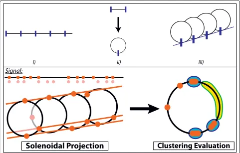
method relies on the fact that the sites that are periodi-cally organized according to a period Ptend to align when the coordinatelis wrapped around aP-periodic solenoid - the solenoids are built as follows: first, the sig-nal support is divided into segments of lengthP; second, the segments are converted into circles (perimeter =P); third, the circles are aligned with respect to the locking up points (Fig. 1). In turn, the site alignments lead to clustering tendencies after a projection onto the face view of the solenoid (Fig. 1). Interestingly, this clustering tendency, or equivalently the tendency for sites to align along the solenoid axis, remains largely unaffected by a small amount of disorder in the positions (noise), by site deletions (false negatives, missing data) or by addition of sites at locations out of phase with respect to the periodi-city (false positives, contaminated data). As a result, the presence of aP-periodic motif can be efficiently detected by using a scoring function that reflects the good cluster-ing properties of the projected sites along the face view of theP-periodic solenoid - hence, the method has been called the solenoidal coordinate method (SCM). In parti-cular, such a method is expected to be robust towards strong signal distortions, as we shall see below. The sole-noidal picture is useful to have an intuitive (geometric) understanding of the method. From a formal point of view, a site at positionxleads to a positionxPon the face view of theP-periodic solenoid, which is simply given by the congruence moduloP, i.e. ×≡xPmodP. As a conse-quence, in the following we will refer the positionsxPto as thepositions modulo P. We shall use the terminology

site modulo Pas well.

Scoring function

The scoring function used here takes into account the self-information [17], or equivalently the information content, that is related to the distances separating the sites modulo P. More precisely, let us call p(xP) the

p-value for any two such sites to be separated by a dis-tancexP, supposing a random uniform distribution of the sites in {1, ...,P}. The scoring function then adds up the information contents [- log(p(xP))] of the nearest sites. Due to the presence of low p(xP)’s coming from both small and large distancesxP, the presence of aP-periodic pattern results in a high scoring function. Geometrically speaking, small distances correspond to dense regions of the solenoid face view and large distances to poor regions (Fig. 2). To summarize, the scoring function at the core of theSCM consists of i) a modulo operation and ii) a cluster analysis of the resulting sites, which rewards both dense and poor regions. In geometrical terms, this can be viewed as i) a solenoidal projection and ii) a cluster analy-sis of the projected sites (Fig. 1).

Solenoidal spectra

therefore consists in computing a spectrum, which is called hereafter the solenoidal spectrum (SoS). The pre-sence of periodic patterns is then revealed by peaks in the spectrum that are exceptionally high. To quantita-tively evaluate the likelihood of the peaks, the scores are interpreted in terms of a p-value. At a given period, this

p-value corresponds to the probability of having a higher score by randomly drawing the sites according to a uniform law. The computation of thep-values gener-ates a p-valued solenoidal spectrum (pSoS). In this regard, supposing that the spectrum is composed ofNp independent peaks, the probabilitypto have more than one spectrum having at least one peak with a p-value lower thanp* reads

p= − −_{1 (1} p∗₎Np_{. (1)}

This allows to quantitatively evaluate the statistical significance of apSoS, though the independence of the peaks, if any, may be a delicate point to prove. In any

case, the probability for such a spectrum to occur by chance is lower than 1− −(1 p∗)Np _.

Identifying the periodic points

In a periodical dataset, all the sites are not expected to be positioned accordingly to the apparent periodicity. In particular, in addition to some wrongly predicted posi-tions, datasets may contain sites that are generated from different sources or that belong to different families (e. g., different families of co-regulated genes). The posi-tions of these sites are therefore not expected to be cor-related. Interestingly, the SCM allows to determine which sites are concerned by a given periodicity. More precisely, a positional score can be defined for each site, which is related to the likelihood for the site to be peri-odically positioned with respect to the other sites of the dataset.

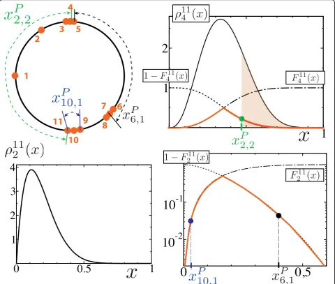
Figure 2Building elements for the scoring function (Eq. 3).Left upper panel: The sites modulo the period are numerated clockwise. Their relative positions depend on the valuePof the period. The normalized (with respect to the periodP) distance between thejthnearest

neighbors on each side ofiis called xi jP, .Right upper panel: Thejthnearest neighbors on each side of any siteiare separated by 2j- 1 sites.

Hence, in order to compute thep-value pN_j (x_{i j}P_,) associated to any distance x_{i j}P_, , one needs the density distribution, respectively the

repartition function, for the distances between sites that are separated by 2j- 1 sites, that is ₂N_j−1 and F2Nj−1 respectively. For anyxÎ0[1],

p

jN

( )

x corresponds to the area of the tails of 2Nj−1 (indicated in brown forN= 11,j= 2 and x =x2 2P, ). For questions of computational

readiness,

p

N_j

( )

x is approximated by min

(

F2N_j−1

( ),

x

1

−

F2N_j−1

( )

x

)

- see Eq. (4) - which is represented by the cuspate red curve.Left

lower panel: The contribution of both x_{10 1}P_, and x_{6 1}P_, is evaluated from the same density function 

1 11

( )x since both distances correspond

P-solenoid face view. The principle consists in rewarding the sites that are located in the dense regions of the solenoid face view. To this end, we use, again, a quantity akin to the information content related to the distances of the nearest neighbors. Each pair of sites on each side of iis allocated with a probabilityp<for the sites to be separated by a distance that is inferior to their current distance, supposing the sites to be randomly drawn according to a uniform distribution. This leads to the information content [- log(p<)]. Next, a scoring func-tion ′( , )i P associated toiat the periodPis defined. It is equal to the maximum information content obtained from the nearest neighbors,i.e. from the pair of nearest neighbors that has the lowestp<.

The higher ′( , )i P , the better the site is positioned according to the periodicity, or equivalently the denser the cluster to which it belongs on the solenoid face view (Fig. 1). The results are quantified by computing the

p-value of ′, hereafter referred to aspv(′). In parti-cular, the positional score ofiat the period Pis defined by:

_pos = −log ( ( ( , ))).₁₀ p_v ′i P (2)

Implementation

Periodic pattern detection: generating the solenoidal spectra

The next paragraph provides some details about the scoring function that is at the core of theSCM. The sec-ond paragraph provides further details about the com-putation of the p-values that are involved in the scoring function.

Scoring function

Let us consider the positions moduloP of a given set of

Nsites. Let us numerate the sites modulo Pby sorting them clockwise (Fig. 2). For such a given sitei, the nor-malized (with respect to the periodP) distance between the two j-th nearest neighbors on each side of i, and hence separated by 2j - 1 sites, is noted xi jP, . We also

call pjN(xi jP,) the correspondingp-value for these sites

to be separated by a distance xi jP, - see next paragraph

for the computation of thep-value, the information con-tent associated to the measurement x_{i j}P_, therefore reads

− ⎡

⎣ log(pNj (xi jP,))⎤⎦. The scoring function scs( )P at the

core of theSoS consists in summing up the information contents over theJ first nearest neighbors around each of theNsites:

_{scs i}N

i j P j J i N P

JN p x

( )= − log( ( _,)).

= = −

∑

∑

1 2 1 0 1 (3)

J represents the maximum number of nearest neigh-bors to be considered. Hence, the computation is all the faster that J is small. However,J must increase with N

in order to efficiently detect dense regions. In this regard, all the reported results in this article have been obtained by choosing J = max(E[N/16], 1) where the function E[x] gives the integer part of x. We have observed that the precise dependence of J on N does actually not affect the detection.

p-values pjN(xi jP,)

For alli andj, p_jN(x_{i j}P_,) is the probability for generating a distance as extreme as x_{i j}P_, when the sites are inde-pendently drawn according to a uniform law. In the case of dense regions, respectively poor regions, this corresponds to generate distances that are smaller, lar-ger respectively, than xi jP, . This can be explicitly written

in terms of the probability density 2Nj−1( )x of the

ran-dom variable associated to the distance between any pair of sites that are separated by 2j-1 sites, which can be readily computed∀jÎ{1,...,N/2} as explained now.

First, the probability _iN

x dx

( ) corresponds to finding one site at a distance x of a given site, andi sites at a distance lower thanx. Next, there areN- 1 possibilities for placing one site at a distancexand _Ni

−2 for placing

iof the remainingN- 2 sites, kl=k l k!(l−!)! standing for the

binomial factor. As a result, _iN

x

( ) reads

_iN

N

i i N i

x N x x

( )=( −1) ₋₂ (1− ) − −2 .

For computational readiness, we use an approximation of thep-value that is valid for both short and large dis-tances, which does not affect the issue of theSCM - see Fig. 2 for an illustrative explanation:

pjN(xi jP,)min(F2Nj−1(xi jP,),1−F2Nj−1(xi jP,)), (4)

where F₂N_j−1 stands for the repartition function

asso-ciated to ₂N_j−1, that is F₂N_j1x xdy ₂N_j1y

0

−( )=

∫

 −( ). Dense

regions correspond to small values of F j x

N i j P

2−1( ,) so that

Eq. 4 leads to the right value of p_jN(x_{i j}P_,) in the limit of

small distances, that is p_jN x F x

i jP Nj i jP

( _,)= 2−1( _,). On the other

hand, poor regions correspond to values of F2Nj−1(xi jP,) close

to 1 so that we also recover pNj(xi jP,)= −(1 F2Nj−1(xi jP,)) in the limit of

large distances. Intermediate values of xi jP, , i.e. close to

the maximum of ₂N_j−1, do not play any crucial role for

Positional score

The positional score is calculated by analyzing the posi-tion of the nearest neighbors moduloP, i.e. the nearest neighbors on the P-solenoid face view. This means to compute thep-valuep<for two sites to be separated by a distance that is inferior to their current distance sup-posing that the sites have been randomly drawn accord-ing to a uniform distribution.

Let us call y_{i j}P_, the distance between any two sites moduloP iandj. Thep<’s are then given by:

p<(yi jP,)=F(Nj i N− + )%N(yi jP,) ∀ ∈i j, { ,1, }N

where % stands for the modulo operator. This leads to

′ = −

{

<

}

( , ) min log( ( ))

, ,

i P p y

j k j k

P

J

where 〈j, k〉J stands for the set of pairs composed of two sites that lie on the J first nearest neighbors on each side ofi.

Results and discussion

Periodic pattern detection

Two methods are often used to highlight the presence of periodic patterns. The first one is mostly used in the case of sparse boolean sequences, which is the case trea-ted here. It consists in computing the histogram of the distances that separate each pair of points. The histo-gram is then analyzed thanks to a (discrete) Fourier transform. The second one is a standard procedure for analyzing continuous signals. It consists in computing an autocorrelation function, which is then analyzed thanks to a Fourier transform, too.

To illustrate the efficiency of the SCM, the pSoS is first compared to the pair-distance histogram technique for different kinds of small sets of positions (Fig. 3). Next, it is compared to the autocorrelation technique for site positions coming from both artificial and real datasets.

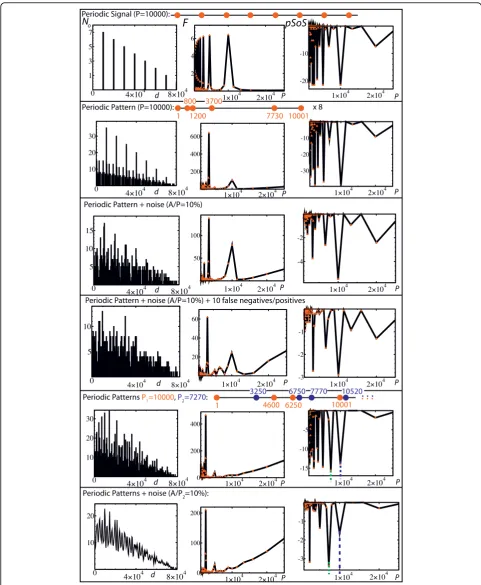
SCM versus pair-distance histograms - Fig. 3

Each row of Fig. 3 corresponds to the analysis of a spe-cific set of positions, which is indicated at the top of the row. The first column gives the pair-distance histograms by reporting the number of occurrenceNoof the dis-tances (bin = 50). The second column gives the discrete Fourier transform F of the pair-distance histogram. Finally, the third column gives thep-value Solenoidal Spectrum (pSoS) using a semi-log scale. The first row shows the equivalence between FandpSoSfor a Dirac comb with periodP = 10000,i.e. a set of sites that are regularly spaced by a distance P= 10000. In both spec-tra, the peaks are harmonics of a main peak (periodP= 10000). The second row shows the results for a set of

positions that consists of a periodic succession (8 times here) of a complex pattern (red points). The period is still 10000. In F, the main peak is obtained at P ~ 10000/6 whereas the pSoSstill provides the main peak at P = 10000 (the other main peaks are harmonics of this period). In the third row, noise is added by drawing the positions according to a uniform distribution of amplitude A, which is centered around the sites of the second row (i.e., the second row corresponds to A= 0). For A/P = 10%, unlike the Fourier transform, most of thepSoS’s still provide a main peak atP= 10000. The fourth row shows the results for the same set of posi-tions as in the third row, except that 10 points (of the 40 initial ones) have been deleted (false negatives) and replaced by 10 points at random locations (false posi-tives). One can see that the SCMis still able to detect the presence of the periodic pattern, which demon-strates the robustness of the method with respect to data contamination.

The last two rows show the results for positions resulting from the combination of two periodic patterns having different periods (blue and red points). In the fifth row, positions correspond to a succession of the periodic motifs up to the position 80000, resulting in 56 points. The Fourier spectrum of the pair-distance histo-gram is flat around one of the main period (P= 10000) whereas all the peaks in thepSoS are harmonics of the two main periods P = 7270 and P = 10000, which are respectively indicated by the green and blue dashed ver-tical lines. The last row gives the curves that result from an average over 100 sets of positions drawn by adding noise to the previous case. In contrast to the Fourier spectrum of the pair-distance histogram, the two main periods are revealed by two sharp peaks in the pSoS, plus one main harmonic peak for each of them.

To summarize, the pair-distance histogram method is poorly efficient to highlight the periodic presence of a complex motif. More strikingly, the mixing of two motifs having two different periods lead to flat Fourier spectra of the pair-distance histograms around the expected periods. On the contrary, even in the presence of noise, the pSoS leads to well-defined peaks that clearly reveal the two different periods.

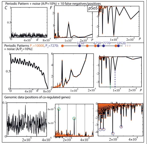
SCM versus autocorrelation function - Fig. 4

The autocorrelation functionC(x) of an infinitely long

sequence X is defined by C x X i X i x

L _i L

L

( )=lim ( )⋅ ( + )

→∞

∑

₌



0

In this case, the autocorrelation function is defined by

C x _{L x} X i X i x

i L x

( )= ₋ ( )⋅ ( + )

= −

∑

  

0

. The SCMis compared to the

autocorrelation method in Fig. 4. The first (second) row corresponds to the case treated in the fourth (sixth) row of Fig. 3. The last row reports the analysis of positions coming from genomic studies.

sizes,...) can be checked to have little, if any, positive impact on the results.

In the last row, 90 genes of the 4639675 base-pair long Escherichia coli genome were analyzed. The posi-tions were taken from the Regulon DataBase [18]. They correspond to the genes that present experimental evi-dence for being transcriptionally regulated by the tran-scription factor CRP, which is the trantran-scription factor that regulates the most genes in E. coli. The Fourier transform of the autocorrelation function leads to two significant high peaks at periods 9508 and 27782 (green circles) whereas the pSoSleads to four significant high peaks at periods 6581, 9507, 19015 and 27782 (blue cir-cles). In particular, the highest peak in the pSoS, i.e. the peak at the period 19015, has no counterpart in the autocorrelation function. These different results would lead to different interpretations of the genomic organi-zation, and hence, to different predictions of the spatial organization of DNA [11].

Positional scores

To illustrate the possibility to identify the periodic sites, we present in Fig. 5 two case studies in the situation of two periodic patterns having two different periods. These correspond to the case studies of the last rows of Fig. 3. Fig. 5a reports the positional score given by Eq. 2 as a function of the site position for noise-free periodic patterns (fifth row of Fig. 3). The blue (red) points give the positional scores of the points at the period 7270 (10000). High scores are obtained at period 7270, respectively 10000, for the points that form the 7270-periodic, 10000-periodic respectively, pattern.

A useful way for distinguishing the points that belong to different periodic trends then consists in plotting the quantity 10–Spos(P)_{,i.e. p}

v(S′(P)) in Eq. 2, computed at the periodP = 10000 versus the same quantity computed at the period P = 7270, which is done in Fig. 5b. In this plot, one can clearly distinguish the points that belong to the 10000-periodicity (points along thex-axis) from Figure 5Positional scores: detecting periodic sites. (a): Positional score as a function of the position of the sites. The analyzed sequence is that of the fifth row of Fig. 3. (b): The x-axis, respectively the y-axis, is given by 10–Spos(P)_=pv(S′_{(P)) (see Eq. 2) computed atP= 7270,P= 10000}

those that belong to the 7270-periodicity (points along the y-axis). Interestingly, this representation also allows to distinguish the different points for a sequence that is distorted. In Fig. 5c, the distortion consisted in adding noise to the sequence used in Fig. 5a and 5b. This was done by drawing the positions according to a uniform distribution of amplitude 727 (i.e. 10% of 7270), which is centered around the original sites. This hence corre-sponds to the situation of the last row of Fig. 3. In con-trast, in Fig. 5d, we report the quantity 10-Spos(P) computed at P = 8700 versus the same quantity com-puted atP = 5300, i.e. at periods where no regularities are expected. In this situation, the points are no more separated.

Conclusion

Pair-distance histograms and auto-correlation functions, either analyzed by discrete or continuous Fourier trans-forms, may be poorly appropriate for highlighting the presence of periodic patterns in sparse and noisy sequences. More importantly, both methods do not suc-ceed in disentangling multiple patterns having different periods so that the corresponding Fourier spectra are flat at the periods supposedly characterizing the sequence (Fig. 3 and 4). In contrast, the solenoid coordi-nate method (SCM) has been built in order to be parti-cularly sensitive to any periodic patterns, even in the case of overlapping patterns with different periods. Its robustness to signal distortion, which can be due to the presence of noise, false positives or/and false negatives, stems from the remarkable alignment properties of peri-odic sites when they are represented in a solenoidal coordinate system with the right period (Fig. 1). It must also be noted that theSCMdoes not need any smooth-ing of the original sequence as in the case of the auto-correlation function. Finally, thanks to the definition of a positional score, we have shown that theSCM frame-work further allows to identify the sites that participate most in a periodic tendency. This should be particularly useful for identifying periodic genes, and hence, for investigating their functional properties.

The present method is suited to sparse (boolean) sequences that contain a rather small number of sites (1’s). More precisely, the computational time for run-ning a spectrum of a sequence contairun-ning Nsites scales as JN~ N2 (see Eq. 3). The method is therefore poorly scalable in its present form. Different improvements along this direction can be contemplated. A possible one would consist in computing the Kullback-Leibler divergence (with respect to a uniform distribution) of the density distribution of the sites modulo the periods,

i.e. the Kullback-Leibler divergence of the density distri-bution along the solenoid face views. This cannot be

done when the number of sites is too small, which was the case treated here.

Availability and requirements

The software is available for public use at http://www. issb.genopole.fr/MEGA/Softwares/iSSB_SolenoidalAppli-cation.zip.

List of abbreviations used

SCM: solenoidal coordinate method;SoS: solenoidal spectrum;pSoS:p-valued Solenoidal Spectrum

Competing interests

The authors declare that they have no competing interests.

Authors’contributions

IJ, JH and FK participated in the design of the study. IJ and JH performed the statistical analysis. IJ, JH and FK wrote the paper. All authors have read and approved the final manuscript.

Acknowledgements

This work was supported by the Sixth European Research Framework (project number 034952, GENNETEC project), PRES UniverSud Paris, CNRS and Genopole.

Author details 1

Institut des Systèmes Complexes Paris Île-de-France, 57-59 rue Lhomond, F-75005, Paris, France.2_{Epigenomics Project, Genopole, CNRS UPS3201,} UniverSud Paris, University of Evry, Genopole Campus 1 - Genavenir 6, 5 rue Henri Desbruères - F-91030 EVRY cedex, France.

Received: 26 March 2010 Accepted: 10 September 2010 Published: 10 September 2010

References

1. Hochschild A, Ptashne M:Cooperative binding of_lrepressors to sites separated by integral turns of the DNA helix.Cell1986,44(5):681-7. 2. Collado-Vides J, Magasanik B, Gralla JD:Control site location and

transcriptional regulation inEscherichia coli.Microbiol Rev1991, 55(3):371-94.

3. Müller J, Oehler S, Müller-Hill B:Repression oflacpromoter as a function of distance, phase and quality of an auxiliary lac operator.J Mol Biol

1996,257:21-9.

4. Korbel JO, Jensen LJ, von Mering C, Bork P:Analysis of genomic context: prediction of functional associations from conserved bidirectionally transcribed gene pairs.Nat Biotech2004,22(7):911-7.

5. Warren PB, ten Wolde PR:Statistical analysis of the spatial distribution of operons in the transcriptional regulation network ofEscherichia coli.J Mol Biol2004,342(5):1379-90.

6. Kolesov G, Wunderlich Z, Laikova ON, Gelfand MS, Mirny LA:How gene order is influenced by the biophysics of transcription regulation.Proc Natl Acad Sci USA2007,104(35):13948.

7. Képès F:Periodic epi-organization of the yeast genome revealed by the distribution of promoter sites.J Mol Biol2003,329(5):859-865.

8. Képès F:Periodic transcriptional organization of theE. coligenome.J Mol Biol2004,340(5):957-964.

9. Wright M, Kharchenko P, Church G, Segrè D:Chromosomal periodicity of evolutionarily conserved gene pairs.Proc Natl Acad Sci USA2007, 104(25):10559.

10. Képès F, Vaillant C:Transcription-based solenoidal model of chromosomes.Complexus2003,1(4):171-180.

11. Junier I, Martin O, Képès F:Spatial and topological organization of DNA chains induced by gene co-localization.PLoS Comput Biol2010,6(2): e1000678.

13. Ghil M, Allen MR, Dettinger MD, Ide K, Kondrashov D, Mann ME, Robertson AW, Saunders A, Tian Y, Varadi F:Advanced spectral methods for climatic time series.Rev Geophys2002,40:1003.

14. Ahdesmäki M, Lähdesmäki H, Gracey A, Shmulevich L, Yli-Harja O:Robust regression for periodicity detection in non-uniformly sampled time-course gene expression data.BMC Bioinformatics2007,8:233. 15. Liang KC, Wang X, Li TH:Robust discovery of periodically expressed

genes using the laplace periodogram.BMC Bioinformatics2009,10:15. 16. Storey JD, Tibshirani R:Statistical significance for genomewide studies.

Proc Natl Acad Sci USA2003,100(16):9440-5.

17. Shannon CE, Weaver W:The mathematical theory of communication. Urbana: University of Illinois Press 1975.

18. Gama-Castro S, Jimenez-Jacinto V, Peralta-Gil M, Santos-Zavaleta A, Penaloza-Spinola M, Contreras-Moreira B, Segura-Salazar J, Muniz-Rascado L, Martinez-Flores I, Salgado H, Bonavides-Martinez C, Abreu-Goodger C, Rodriguez-Penagos C, Miranda-Rios J, Morett E, Merino E, Huerta A, Trevino-Quintanilla L, Collado-Vides J:RegulonDB (version 6.0): gene regulation model ofEscherichia coliK-12 beyond transcription, active

(experimental) annotated promoters and Textpresso navigation.Nucleic Acids Research2007 [http://nar.oxfordjournals.org/cgi/content/full/ gkm994v1], gkm994v1.

doi:10.1186/1748-7188-5-31

Cite this article as:Junieret al.:Periodic pattern detection in sparse boolean sequences.Algorithms for Molecular Biology20105:31.

Submit your next manuscript to BioMed Central and take full advantage of:

• Convenient online submission

• Thorough peer review

• No space constraints or color figure charges

• Immediate publication on acceptance

• Inclusion in PubMed, CAS, Scopus and Google Scholar

• Research which is freely available for redistribution