R E S E A R C H
Open Access
The effect of parameter variability in the
allometric projection of leaf growth rates
for eelgrass (
Zostera marina
L.) II: the
importance of data quality control
procedures in bias reduction
Héctor Echavarría-Heras
1*, Cecilia Leal-Ramírez
1, Enrique Villa-Diharce
2and Nohe R. Cazarez-Castro
3* Correspondence: [email protected]
1Centro de Investigación Científica y
de Estudios Superiores de Ensenada, Carretera
Ensenada-Tijuana No. 3918, Zona Playitas, Código Postal 22860, Apdo. Postal 360 Ensenada, B.C., Mexico Full list of author information is available at the end of the article
Abstract
Background:Eelgrass grants important ecological benefits including a nursery for waterfowl and fish species, shoreline stabilization, nutrient recycling and carbon sequestration. Upon the exacerbation of deleterious anthropogenic influences,
re-establishment of eelgrass beds has mainly depended on transplantation. Productivity estimations provide valuable information for the appraisal of the restoration of ecological functions of natural populations. Assessments over early stages of transplants should preferably be nondestructive. Allometric scaling of eelgrass leaf biomass in terms of matching length provides a proxy that reduces leaf biomass and productivity estimations to simple measurements of leaf length and its elongation over a period. We examine how parameter variability impacts the accuracy of the considered proxy and the extent on what data quality and sample size influence the uncertainties of the involved allometric parameters.
Methods:We adapted a Median Absolute Deviation data quality control procedure to remove inconsistencies in the crude data. For evaluating the effect of parametric uncertainty we performed both a formal exploration and an analysis of the sensitivity of the allometric projection method to parameter changes. We used parameter estimates obtained by means of nonlinear regression from crude as well as processed data. Results:We obtained reference leaf growth rates by allometric projection using parameter estimates produced by the crude data, and then considered changes in fitted parameters bounded by the modulus of the vector of the linked standard errors, we found absolute deviations up to 10 % of reference values. After data quality control, the equivalent maximum deviation was under 7 % of corresponding reference rates. Therefore, the addressed allometric method is robust. Even the smaller sized samples in the quality controlled dataset produced better accuracy levels than the whole set of crude data.
(Continued on next page)
(Continued from previous page)
Conclusions:We propose quality control of data as a highly recommended step in the overall procedure that leads to reliable allometric surrogates of eelgrass leaf growth rates. The proliferation of inconsistent replicates in the crude data points towards the importance of discarding incomplete leaves. We also recommend avoiding errors in estimating the biomass of small leaves for which precision of the used analytical scale might be an issue.
Keywords:Eelgrass leaf growth rates, Allometric estimation, Parametric uncertainty effects, Data quality control
Background
Eelgrass is a relevant seagrass species that distributes worldwide in estuaries and near-shore environments. Eelgrass meadows provide habitat and foraging grounds for marine animals, buffers the shoreline from erosion, filter the water, and oxygenate the sediments. Recently at a global scale, deleterious effects derived from anthropogenic influences, have been exacerbated to such an extent that in the absence of remediation efforts, the import-ant ecological services resulting from the permanence of eelgrass meadows could be irre-versibly lost. Due to its ecological relevance eelgrass has been the subject of intense research and conservation efforts that are mainly carried out by means of transplanting plots. The measurement of biomass and productivity, provide key information for the evaluation of the overall status of a given eelgrass population. The noticeable growth form of this species makes the average rate of leaf growth per shoot-day measured over a grow-ing interval of lengthΔtdeterminant of overall productivity. In what follows we denote the biomass of an individual eelgrass leaf at timetthrough the symbolw(t) and its corre-sponding length by means ofl(t). Similarly, we will symbolize the observed values of the biomass of leaves in shoots by means of ws(t) and the average rate of leaf growth per
shoot-day through Lg(t, Δt). Conventional techniques for the assessment of Lg(t, Δt), require intensive sampling that involves the removal of shoots, and then tedious, time consuming dry weight measurement procedures in the laboratory. Even though the elim-ination of eelgrass shoots linked to a typical evaluation activity does not infringe damage to natural populations, the effects of shoot removal could be severe for transplanted plots. Therefore, in an overall program that leads to eelgrass conservation it is important to in-clude nondestructive assessment methods [1, 2].
Bivariate allometric scaling relationships between measured quantities X and Y
expressed as a power function of the form Y=βXα, appear in a myriad of research problems in physics, biology, and earth and planetary sciences [3–11]. The parameterα is named allometric exponent and β termed normalization constant. Particularly, Echavarria-Heras et al. [1] and Echavarria-Heras et al. [2], stressed the significance of the model
w tð Þ ¼βl tð Þα; ð1Þ
in the adaptation of an allometric proxy for Lg(t,Δt). This allometric surrogate will be here denoted by means of the symbolLga(α, β, t, Δt), and its explicit formulae derived inAppendix A.
site could be used to readily obtain surrogates for currently observed values of Lg(t,Δt) Several studies show that within our geographical region the parameters αandβcan be considered as time invariant ([1, 11–14]). But even thoughαandβare statistically invariant within a given region, environmental influences are expected to induce a relative extent of variability on local estimates of αandβ[11] and as it was stated by Echavarria-Heras et al. [2] this could propagate significant uncertainties onLga(α,β,t,Δt)
values. Indeed the results of Appendix B corroborate that these proxies could produce sig-nificantly accurate assessments forLg(t,Δt) only in case the fitting of equation (1) yields highly precise estimates of the parametersαandβ.
One important factor contributing to the uncertainty of the estimates of the parame-ters α and β, in equation (1) associates to the set of biological influences that could have been disregarded when assuming that eelgrass leaf biomass depends solely on linked length. Another important source of uncertainty relates to the failure of the model of equation (1) to handle environmental effects on a proper way. But the high values of determination coefficients as well as results of residual analysis corresponding to fittings of the model of equation (1) to independent data sets collected in our geographical region ([1, 2, 11, 13, 15, 16]) reveal that on spite of its simplicity, equation (1) is a para-digm that provides highly consistent estimates of the involved parameters.
Eelgrass leaf biomass is lognormally distributed, and the sizes of the different groups of replicates that make up our data are reduced. Therefore, we removed inconsistent replicates from the set of crude data by using a robust median absolute deviations cleaning procedure. We also relied on a sensitivity analysis study in order to assess the improvement in the accuracy of the Lga(α, β, t,Δt) proxy that may possibly be
associ-ated to whatever reduction on the uncertainties of αand βcould be derived from an improvement in data quality. Besides, we explored the corresponding effects of sample size, by randomly drawing differently sized samples out of both the crude and the proc-essed data sets and then comparing the values of the determination coefficients for the fittings of equation (1) to the selected samples. In the Methods section we further sub-stantiate the data cleaning approach, the procedure for estimating the effects of sample size as well as the steps of the performed sensitivity analysis. In the Results and Discus-sion section we elaborate on the relevance and limitations of this study. In the Conclu-sions section we presented the summary and potential implications of our findings.
Methods
Raw data
For the aims of the present research we assembled an extensive data set containing mea-surements taken on a total of 10412 individual eelgrass leaves collected in San Quintin Bay Baja California as previously reported in ([1, 2, 11–14]). Crude data includes measure-ments of length (mm), width (mm) and dry weight (gr).
Data quality control procedures
Short [21] and Gaeckle and Short [22] estimated leaf biomass in eelgrass by using an iso-metric weight to length ratio, and the appropriateness of alloiso-metric methods in eelgrass research has been validated for a number of independent data sets (e.g. [1, 2, 11–16] and references therein). Particularly, Echavarria-Heras et al. [2] formally demonstrated that the conspicuous leaf architecture and growth form of eelgrass makes leaf length a reliable allometric descriptor of the associated biomass. Indeed, results show that for independent data sets collected in our geographical region the model of equation (1) always produced reliable fits ([1, 2, 11–13, 15, 16]). Moreover, the results of Solana-Arellano et al. [11] stat-ing that the parameters associated to the scalstat-ing relationship of equation (1) can be con-sidered invariant within a given geographical region, endorse that this model is highly consistent. This makes it reasonable to assume that the true relationship linkingw(t) and
biological influences or local environmental forcing. Moreover, by using a direct sur-vey of the dispersion pattern shown by the present crude data (Fig. 1) we observed that departure of a given replicate from an expected power function-like trend was more pronounced for leaves with smaller sizes. Since, this effect was not observed in related data sets collected in our region, we judged that these inconsistencies could be in a fundamental way tied to the considerably larger extension of the present data set, which required processing performed by several technicians and it was perhaps a lack of standardization in these tasks that explains the present proliferation of incon-sistencies that should be removed in order to prevent their permanence from exerting a reduction in the precision of estimates for the parameters in the scaling relationship of equation (1). Notwithstanding, the judgment to remove an outlier or inconsistent measurement in a data set, it is necessary to be able to identify its occurrence. Data clean-ing procedures tasks are commonly performed by usclean-ing a mean plus or minus three standard deviations method. This technique is based on the property of a normal distribu-tion for which 99.87 % of the data appear within this range [23], but its applicadistribu-tion in the present settings presents difficulties. It firstly assumes that the distribution of data is normal while eelgrass leaf biomass is lognormally distributed [2]. Secondly, both the mean and standard deviation are strongly impacted by outliers [24]. Thirdly, our data is com-posed by groups of measurements that include a reduced number of leaf biomass repli-cates, and the mean plus or minus three standard deviations method is very unlikely to detect outliers in small samples [25]. This fact made it also inconvenient to use alternative data cleaning techniques like studentized residuals, the hat elements, Cook’s distance, or the Mahalanobis distance procedure [26]. Alternatively, the median of a group of data is totally immune to the sample size and a robust estimator of scale, reason why we adapted a Median Absolute Deviation (MAD) method [27] which provided the present criteria for the removal of inconsistencies in groups of more than 10 replicates of biomass values associated to a given leaf length. By eliciting the consistency of the allometric scaling of equation (1), we assumed that the addressed length-to-weight variation pattern should conform to a power function-like trend Therefore, individual leaf biomass measurements
that in an initial data analysis were found to severely deviate from this pattern in sets under 10 replicates were removed from the set of unprocessed data. In summary, by ana-lyzing the spreading of leaf biomass values in a leaf length-to-weight plot, we detected replicates that we supposed represented unduly deviations from an expected power function-like variation pattern. By applying the explained data cleaning procedures we re-moved these from the set of crude data, because in light of the proven consistency of the scaling relationship of equation (1) these inconsistent replicates could have been caused by errors due to a lack of standardization in leaf length or biomass measurements, or per-haps, explained by errors owed to faulty equipment for dry weight assessment or even ex-plained by incorrect recordings.
In order to formalize the present MAD data cleaning procedure, we arranged the crude data in different groupsG(l) = {wG1(l),…,wGn(l)} formed by an observed leaf lengthland
associated leaf biomass replicateswG1(l),…,wGn(l). For almost all groups of replicatesG(l)
we observed several leaf biomass values that parted from the expected variability pattern and were considered as inconsistencies. For each groupG(l) we firstly obtained its median denoted by means of the symbolMED{wG1(l),….,wGn(l)} or simply by means ofM(G(l))
for short. Then, for each replicatewGj(l) in (G(l) we calculated its absolute deviation from
the group median δGj(l), that is, δGj(l) = |wGj(l)−M(G(l))|. Similarly, we obtained the
median of the set of absolute deviations denoted by the symbol MED{ δG1(l),…,δGn(l)}.
Following, Huber [28] and also recalling that eelgrass leaf biomass values are log-normally distributed [2], we obtained the Median Absolute Deviation of a groupG(l) de-noted here throughMAD(G(l)) and given by
MAD G lð ð ÞÞ ¼bMEDfδG1ð Þl ;…;δGnð Þl g; ð2Þ
whereb= 1/Q(0.75), beingQ(0.75) the 0.75 quantile of the lognormal distribution. For the removal of inconsistent replicates in a group G(l) we used the decision criterion
M G lð ð ÞÞ−T⋅MAD G lð ð ÞÞ<wjð Þl <M G lð ð ÞÞ þT⋅MAD G lð ð ÞÞ; ð3Þ
where T is the rejection threshold that following Miller [24], we set at a value of
T= 3. For groupsG(l) under ten replicates we applied a direct data cleaning procedure by removing replicates that we considered were severely deviated from the central power function-like trend.
Sensitivity analysis
In order to evaluate the influences that the uncertainties of the parametersαandβconvey in the performance of Lga(α, β, t,Δt), we used both a formal study and also simulation
runs. The analytical exploration is presented in Appendix B. For the simulation study, ini-tially, at equally spaced iteration (i.e., sampling) timest, we drawn uniformly distributed random numbers representing a number of shoots retrieved NS(t, Δt) and the number
newly produced leaves. Subsequently, we utilized the simulated leaf lengths and esti-mates α^ and ^β of the parameters α and βin equation (1), in order to produce the proxy growth rates Lga(α,β,t, Δt). In order to produce estimates ^α andβ^ for the
pa-rameters α andβ we followed Hui and Jackson [18], Packard and Birchard [19] and Packard and Boardman [20] and fitted equation (1) to the present data sets using an iterative nonlinear least-squares method rather than the traditional approach of lin-earizing the equation through a logarithmic transformation of data. All fittings were performed using the Matlab Statistics Toolbox.
To study the sensitivity ofLga(α,β,t,Δt) to changes in the parametersαandβwe
se-lected as reference values the estimates α^ andβ^ and produced changing valuesαepfor ^α
andβeqforβ^namely,
αep¼ ^αþΔαp; ð4Þ
βeq¼^βþΔβq; ð5Þ
with the valuesΔαpandΔαqsatisfying
Δαp ¼p⋅stdeð Þα^ ð6Þ
and
Δβq
¼q⋅stdeð^βÞ; ð7Þ
where stdeð Þα^ and stdeðβÞ^ stand for the standard errors of α^ and^β respectively andp
andqare numbers satisfying, 0 <p≤1 and 0 <q≤1.
Therefore, the fluctuating valuesαep andβeqfor α^ and β^ are scaled through
propor-tions pand q of their standard errors. In our analysis we also relied on a parameter change index denoted by means ofρ(p, q), and defined through
ρðp; qÞ ¼
ffiffiffiffiffiffiffiffiffiffiffiffiffiffiffiffiffi
ð
β^−βeqÞ
2 qþ ^α−αep
2
: ð8Þ
Particularly, the maximum value that ρ(p, q) can attain as p and q vary is denoted through the symbolρmax(p,q) and is given by,
ρmaxðp;qÞ ¼
ffiffiffiffiffiffiffiffiffiffiffiffiffiffiffiffiffiffiffiffiffiffiffiffiffiffiffiffiffiffiffiffiffi
steð Þα^ 2þsteð^βÞ2
q
ð9Þ
In what follows we will also use the mean value of ρ(p, q) denoted here byρav(p, q)
and given by
ρavðp;qÞ ¼
ffiffiffiffiffiffiffiffiffiffiffiffiffiffiffiffiffiffiffiffiffiffiffiffiffiffiffiffiffiffiffiffiffiffiffiffiffiffiffiffiffiffiffi
stdeð Þα 2þstdeð Þβ 2=2
q
: ð10Þ
The simulated leave lengths l(t +Δt), corresponding incrementsΔl theNS(t,Δt) and
nl(s) values, and the parameter estimatesα^ andβ^ produced by means of equation (17) a reference trajectory Lgaα^;^β;t;Δ;t. It turns out that every picked value of ρ(p, q)
yields different pairs (αep,βeq), each one associated to a couple (Δαp,Δβq) that comply
with the condition of equation (8). For each pair(αep,βeq), the simulated leave and shoot
that these trajectories produce at each sampling time tis then calculated and its value denoted through〈Lga(αep,βeq,t,Δt)〉ρ. Following the procedure, requires to calculate the
deviations between〈Lga(αep,βeq,t,Δt)〉ρand Lga ^α;^β;t;Δt
, that are denoted by means of the symbolδLgaρ(αep,βeq,t,Δt) and obtained through,
δLgaρ αep;βeq;t;Δt
¼ Lga αep;βeq;t;Δt
D E
ρ−Lga α^; ^β;t;Δt
: ð11Þ
We also need to compute the average through time of theδLgaρ(αep,βeq,t,Δt) deviations
whose output is represented here through the symbol 〈δLgaρ(αep,βeq,t,Δt)〉t. Finally,
it is necessary to obtain the time average of the values of the reference trajectory
Lga α^;β^;t;Δt
. The resulting record is denoted using the symbol Lga ^α;β^;t;Δt
D E
t.
These statistics are then used to produce the relative deviation index ϑ(Δαp, Δβq)ρ
given by
ϑ Δαp; Δβq
ρ¼
δLgaρ αep; βeq;t;Δt
D E
t
Lga α^; β^;t;Δt
D E
t
: ð12Þ
The value of ϑ(Δαp, Δβq)ρ provides a measure of the sensitivity of the reference
trajectory Lgaðα^;^β;t;ΔtÞto a change of toleranceρ(p, q) on the pair (^α, ^β). Moreover,
by calculatingϑ(Δαp,Δβq)maxdefined through, ϑ Δαp; Δβq
max ¼maxρ ϑ Δαp; Δβq
ρ
; ð13Þ
we can get in what percentage of 〈Lgaðα^;β^;t;ΔtÞit the maximum absolute deviation
betweenLga(αep,βeq,t,Δt) andLgað^α;^β;t;ΔtÞamounts.
Sample size effects
In order to explore the extent of sample size influences on Lgaðα^;β^;t;ΔtÞ we
performed the fitting of equation (1), using differently sized samples of leaf length and biomass (l(t),w(t)) data which were randomly drawn from the available datasets. For each sample of size n, we obtained the determination coefficient (rn2) as well as
the values of the estimators of the parameters α^n and ^βn, their respective standard
errors stdenð Þα^ and stdenðβÞ^ and the values of the upper bound ρmax(p,q)n and
ϑ(Δαp,Δβq)ρmax.
Results and discussion
In seagrass research, allometric equations have provided useful empirical models aimed to the representation of biologically relevant traitsYin terms of an easily measured variable
leaf biomass evaluations [15] and have also endorsed the substantiation of the plasto-chrone method of leaf growth assessments [16]. Moreover, equation (1) is the foundation of the derivation of theLga(α,β,t,Δt) proxy of equation (17) a paradigm aimed to the
in-direct assessment of eelgrass leaf growth rates ([1, 2, 12]).
The effectiveness of the Lga(α,β, t,Δt) construct for providing truly accurate and
non-destructive assessments for the observed average rate of leaf growth per shoot-dayLg(t,Δt)
depends on both, the time invariability of the parametersαandβ, and on the accuracy of their estimates. From a general standpoint, the variability of the allometric exponent αhas been the focus of theoretical and empirical studies because it often seems to have a con-stant value specific to a particular biological relationship (e.g. [34–39]). On the other hand, several studies have provided evidence that support certain variability in the exponent of allometric scaling laws (e.g. [40–45]). Accordingly, the value of the normalization constant
βis thought to be characteristic of species or populations [46]. And the variability observed in the normalization constant, explained as a differential response to environmental condi-tions [34, 35, 47–49]. Particularly, for eelgrass, Solana-Arellano et al. [11] analyzed inde-pendent data set collected in different geographical regions to conclude that no universal values can be found for the allometric parameterαin equation (1), suggesting as well that this scaling relationship might be considered static, thus implying that local factors deter-mine the extent of the variability of the actual values of the parameters αandβ. On the presence of this variability associated uncertainties are expected to spread inaccuracies in eelgrass leaf growth rates produced by means of equation (17).
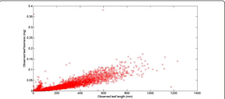
Figure 1 displays the variability of observed leaf lengths and linked biomasses. The sur-vey of the crude data reveals a notorious proliferation of replicates associated to an ob-served leaf length. Data was arranged into 755 different groups G(l) = {wG1(l),…,wGn(l)}.
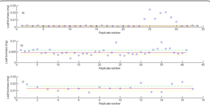
Figure 2 displays the variation of the number of replicates for a given leaf size. We can ob-serve that the number of replicates in groupsG(l) decreases with leaf size. This is probably due to the fact that separation from shoots by drag forces is more pronounced for longer and older leaves than it is for small and younger leaves. Figure 3 shows examples of the dispersion withinG(l) groups. Moderated differences in replicated leaf biomass values as-sociating to a given length can be explained by the inherent stochastic variability along with normal systematic errors introduced by data processing. Nevertheless, an exploration of the dispersion pattern of leaf biomass values in the present crude data reveals replicates representing unduly deviations from the expected power function-like trend. These incon-sistent measurements are more visible for leaves under 100 mm long and also for those longer than 800 mm. For groups with 10 or more replicates and according to the present MAD data quality control criterion, whenever an individual leaf biomass replicate wGj(l)
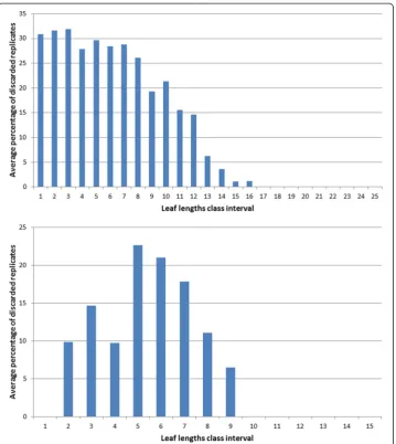
both data sets. For each one of the lengths of in these class intervals we applied the present MAD procedure and calculated the percentage of discarded replicates. Then we obtained the average percentage of discarded leaves that associate to each length class interval. Figure 5 compares the average percentages of discarded replicates per leaf length class for the present data and for the Echavarria-Heras et al. [12] data set. For leaf lengths lying in the first class interval (0≤l(t) < 50) the average percentage of rejected replicates in the present data set was 30 % while the Echavarria-Heras et al. [12] data reported no in-consistent replicates for the same interval. And generally, the percentages of discarded replicates in the present data set were markedly bigger than those associated to the Echavarria-Heras et al. [12] data. This comparison can explain why the fitting the model
Fig. 2Leaf lengths and numbers of associated leaf biomass replicates. The distribution of the number of replicates of leaf biomasses for a given length decreases with leaf length. Maximum number of replicates was 107 and corresponded to a leaf length of 3 mm
of equation (1) to the present crude data set produced an smaller determination coeffi-cient than that reported in Echavarria-Heras et al. [12].
Observations show that the order relationship 0 <β<αholds [1, 2, 11, 12] and that it is also reasonable to consider the variation ranges ofΔαandΔβsatisfying: |Δα| <αand |Δβ| <β. By embracing these assumptions in Appendix B we derived explicit formulae for the deviationsδLga(Δα,Δβ,t,Δt) that changed values of the parametersαandβ
hav-ing the form αe=α+Δα andβe=β+Δβinduce in the reference valuesLga(α,β, t, Δt).
These are given by equations (21). By assuming that the observed order relationship for the parameters α and β holds and also by considering the aforesaid expected variation ranges for Δα and Δβ, we found that the proxies Lga(α, β, t, Δt) for the
average rate of leaf growth per shoot-day, will be overestimated by Lga(αe, βe, t, Δt)
values, primarily when the ordered pair (Δα,Δβ) lies on the domainΔα> 0 andΔβ> 0. Nevertheless, as it is explained in Appendix B, each positive value of Δβ, can be associated to a set of negative values of Δα for which Lga(α, β, t, Δt) will be also
overestimated by Lga(αe, βe, t, Δt). Correspondingly, Lga(αe, βe, t, Δt) underestimates
Lga(α, β, t, Δt) whenever the pair (Δα, Δβ) is placed inside the region -α<Δα< 0
and -β<Δβ< 0, but this time, each value ofΔβsatisfying -β<Δβ< 0 can be associated to a set of positive values ofΔβfor whichLga(α,β,t,Δt) will be also underestimated by
Lga(αe,βe,t,Δt).
By fitting of equation (1) to the crude leaf length and weight data we obtainedr2= 0.81 and estimates,α^¼1:32367 withstdeð Þ ¼α^ 0:0143 forαand ofβ^¼0:000014 withstde ðβÞ ¼^ 1:4e−6 for β. Therefore, according to equation (8) we have 0≤ρ(p,q)≤0.0143. Using the α^ and ^β estimates we obtainedρmax(p,q) = 0.0143 (cf. Eq. (9)) andρav(p,q) =
0.0072 (cf. Eq. (10)). By means of the simulated leave and shoot data and equation (17) we estimated the Lgaðα^; β^;t;ΔtÞ reference trajectory. Afterwards for fixed values of the
parameter change indexρ(p,q) we used equations (6) and (7) to produce values for the
ΔαpandΔβpincrements complying with the condition of equation (8). This allowed the
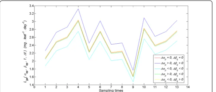
characterization of the associated Lga(αep, βeq, t, Δt) trajectories. Figure 6 displays
trajectories obtained for the case in whichρ(p,q) takes its average valueρav(p,q). These
simulation outputs are consistent with the results of the appendix setting domains of
variation of the pair (Δα, Δβ) where Lga(α, β, t, Δt) values are overestimated or
underestimated. Similarly, Fig. 7 shows the time variation of the average deviations
〈δLga(Δαp, Δβq,t,Δt)〉ρ obtained for ρ(p, q) =ρav(p, q). Moreover, Fig. 8 shows that
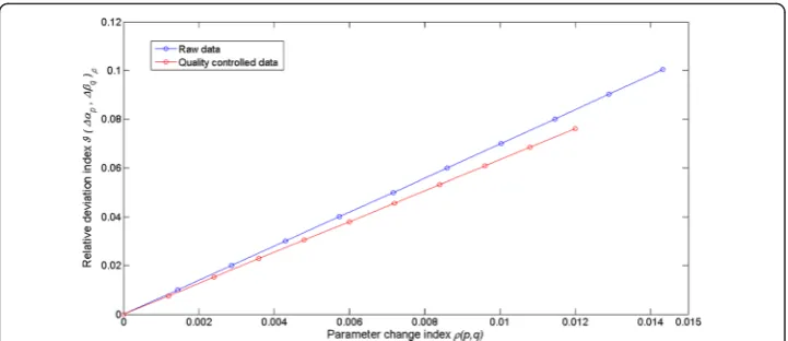
whenever 0≤ρ(p,q)≤ρmax(p,q) the values of the relative deviation indexϑ(Δαp,Δβq)ρare
bounded above by a valueϑ(Δαp,Δβq)max= 0.01, that is, the maximum absolute deviation
betweenLga(αep, βeq, t, Δt) and Lgaðα^; β^;t;ΔtÞ amounts to 10 % of 〈Lgað^α; β^;t;ΔtÞit.
In turn, when fitting of equation (1) to the quality controlled data we obtained
r2= 0.91 and estimates ^α¼1:403 with stdeð Þ ¼α^ 0:0120 forαand of ^β¼8:462e−006
with stdeð^βÞ ¼6:4300e−007, for β. Therefore, according to equation (9) this time we haveρmax(p,q) = 0.01. In turn, performing the sensitivity study of equations (4) through
(13) we obtainedϑ(Δαp,Δβq)max= 0.07, which amounts to 7 % of〈Lgaðα^; β^;t;ΔtÞ〉t (see
Fig. 9).
This sensitivity exploration, sets the accuracy of the allometric method of equation (17) to be mainly dependent on the extent of the upper boundρmax(p,q) of the
param-eter change index ρ(p, q), This means that an improvement in the quality of the fit of equation (1) reducing the magnitude of the upper bound for ρ(p, q) will certainly increase the accuracy of the proxies Lga(α,β, t, Δt). This study also demonstrates the
Fig. 6Examples of deviations between allometrically projected leaf growth rates. We portrait several trajectories of allometrically projected leaf growth ratesLga(αep,βeq,t,Δt) in units of mg. leaf−
1
.day−1. These trajectories were produced by variationsαepandβepin fitted parameters^αand^β, complying with the conditionρ(p,q)2=stde(^α)2+stde(β^)2/4. We show the reference trajectoryLgaðα^;β^;t;ΔtÞin red. The number of days elapsed between sampling times is 15
importance of data quality control in the reduction ofρmax(p,q). Therefore, within the
realm of parametric uncertainties as determined by of the values of stdeð Þ^α and stdeðβÞ^ obtained for the quality controlled data set, the addressed projection method can be considered robust relative to numerical differences in the estimators^αand^β.
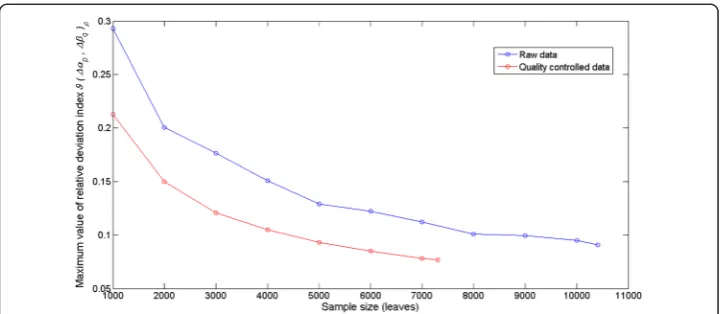
Figure 10 presents the variation of ϑ(Δαp, Δβq)max depending on sample size for
both the set of raw data and that resulting after quality control procedures. As ex-pected Fig. 10 shows that for both data sets ϑ(Δαp,Δβq)maxdecreases as sample size
increases, but these plots also reveal that the effect of sample size on the accuracy of theLga(α,β,t,Δt) proxy is more pronounced for the raw data set. Moreover, even the
Fig. 8The behavior of the relative deviation indexϑ(Δαp,Δβq)ρ. This plot shows the behavior of the relative deviation index for different values ofρ(p,q). This indexϑ(Δαp,Δβq)ρis obtained by dividing the absolute value of the average through time of the deviations between the〈Lga(αep,βeq,t,Δt)〉ρand Lgaðα^;β^;t;ΔtÞrates, by the time average of theLgað^α;β^;t;ΔtÞvalues, (cf. Equation (12)). The relative deviation indexϑ(Δαp,Δβq)ρprovides a measure of the sensitivity of the allometric methodLga(α,β,t,Δt) to changes in the parametersαandβ. The values of the relative deviation indexϑ(Δαp,Δβq)ρare bounded above by a valueϑ(Δαp,Δβq)max= 0.01. (cf. Equation (13))
smallest sized sample in the quality controlled data set (n= 1000) produces a smaller value forϑ(Δαp,Δβq)maxthan that induced by the largest sized sample in the raw data
set (n= 10412). This adds on to the aforesaid on the prominent role of data quality control in improving the accuracy of eelgrass leaf growth rate assessments obtained by means ofLga(α,β,t,Δt).
Conclusions
The results of the present study highlight the important role that the precision of par-ameter estimates linked to the allometric model of equation (1) plays in the overall suitability of the allometric proxy for eelgrass leaf growth rates Lga(α, β, t, Δt) given
by equation (17). The basic allometric model of equation (1) has been consistently identified using different data sets, and a property of invariance for the involved pa-rameters statistically verified. But on spite of model consistency, the evaluation of the extent on what factors such as data quality sampling size, and analysis method can in-fluence parameter estimates is an important entry in the comprehensive analysis of an allometric scaling relationship like equation (1). Moreover, the recommendation by Hui and Jackson [12] stating that for variables that are measured with errors, it is im-portant to obtain accurate estimates with repeated measurements on similar individ-uals grown under similar conditions highlights the relevance of controlling factors that could affect data quality in our settings. Since the present results were obtained following the recommendation of Hui and Jackson [18], Packard and Birchard [19] and Packard and Boardman [20] concerning analysis method, and since sample size in our study was optimal, it is reasonable to assume that errors in data processing could explain a drop in the determination coefficient for the fitting of equation (1) to crude data collected at our study site from R2= 92 obtained by Solana-Arellano et al. [11] and Echavarria-Heras et al. [15] to a value of R2= 81 produced by the present data set. And the fact that after the data cleaning procedures performed on the present data we obtained for the resulting determination coefficient a value of R2= 91 seems
to endorse our judgment. Therefore, our results seem to confirm that data quality can be raised as a crucial factor explaining precision of estimates for the parameters α and βin equation (1). Moreover, the present data quality control procedure reveals the remarkable influence of inconsistencies in reducing precision of allometric projec-tions. Indeed, as it is shown in Fig. 9 the accuracy of the Lga(α, β, t, Δt) proxy
Appendix A
In what follows a subscript s will be used to label a generic eelgrass shoot, holding a numbernl(s) of leaves with combined biomassws(t). In time, ifΔwl(t,Δt) stand for the
increment in biomass that is gained by an individual leaf over a growing interval [t,t+
Δt], then denoting by means ofLsg(t,Δt) the resulting average growth rate of the leaves
on the shootswe will have,
Lsgðt;ΔtÞ ¼ X
nl sð ÞΔwlðt;ΔtÞ
Δt ;
and consequently if Lg (t, Δt) denotes the linked average rate of leaf growth per
shoot-day, we then have,
Lgðt;ΔtÞ ¼
X
N S tð;ΔtÞLsgðt;ΔtÞ
N S tð;ΔtÞ ; ð14Þ
where ∑NS(t,Δt) indicates summation of the shoots collected over the marking interval
[t,t+Δt] and beingNS(t,Δt) their number. Moreover, as it is thoroughly explained by Echavarría-Heras et al. [2], we can use equation (1) in order to derive an allometric ap-proximation forLsg(t,Δt), which we here denote through the symbolLsga(α,β,t,Δt) and
formally express by
Lsgaðα;β;t;ΔtÞ ¼ X
nl sð ÞΔwlaðt;ΔtÞ
Δt ; ð15Þ
whereΔwla(t,Δt) is an allometric proxy forΔwl(t,Δt).
It turns out that equation (1) yields,
Δwlaðt;ΔtÞ ¼ βl tð þΔtÞα−βl tð Þα
then, factoringl(t+Δt)αand taking into account thatl(t +Δt) =l(t)+ΔlwhereΔlstands for the increment in leaf length gained over the interval [t,t+Δt] we get,
Δwlaðt;ΔtÞ ¼βl tð þΔtÞα 1− 1−ρlðt;ΔtÞ
α
where
ρlðt;ΔtÞ ¼ Δl l tð þΔtÞ:
And by letting
δðt;ΔtÞ ¼1−1−ρlðt;ΔtÞα
we equivalently have
Δwlaðt;ΔtÞ ¼ βl tð þΔtÞαδðt;ΔtÞ:
Therefore, from (15) we obtain,
Lsgaðα;β;t;ΔtÞ ¼ X
nl sð Þβl tð þΔtÞ αδ
t;Δt ð Þ
Δt ð16Þ
Lgaðα;β;t;ΔtÞ ¼ X
NS tð;ΔtÞLsgaðα;β;t;ΔtÞ
NS tð ;ΔtÞ ; ð17Þ
and in turn we have
Lgðt;ΔtÞ ¼ Lgaðα;β;t;ΔtÞ þ∈ga; ð18Þ
with the term ϵga standing for the involved approximation error. It is worth to point out that the derivation of the results of equation (18) could have been done using leaf areaa(t) in place ofl(t).
Appendix B
In this appendix we firstly derive explicit formulae for the deviationsδLga(Δα,Δβ,t,Δt)
that a change Δαand Δβin αand β will induce inLga(α, β, t, Δt). Using the derived
forms we obtain domains of variation ofΔαandΔβwhereLga(α,β,t,Δt) are
underesti-mated or overestiunderesti-mated. Without loss of generality, we will assume through that the in-equality 0 <β<αholds, as it regularly occurs in fittings of equation (1) to eelgrass leaf biomass and length data. Also, for the sake of mathematical tractability, without sacri-ficing pertinence of the analysis, regarding the increments Δαand Δβ we will assume that |Δα|≤αand |Δβ| <β.
By definition above we have,
δLsgaðΔα; Δβ;t;ΔtÞ ¼LsgaðαþΔα; βþΔβ;t;ΔtÞ−LsgaðΔα; Δβ;t;ΔtÞ ð19Þ
And from equation (17) one gets
δLgaðΔα;Δβ;t;ΔtÞ ¼ X
NS tð;ΔtÞδLsgaðΔα; Δβ;t;ΔtÞ
NS tð;ΔtÞ ð20Þ
Now equation (16) yields,
δLsgaðΔα; Δβ;t;ΔtÞ ¼ X
nl sð Þβl tð þΔtÞ
αδðt;ΔtÞμ
LgðΔα;Δβ;l tð þΔtÞÞ
Δt ; ð21Þ
With
μLgðΔα;Δβ;l tð ÞÞ ¼
βþΔβ β
1− 1− Δl
l tð þΔtÞ
αþΔα!!
δðt;ΔtÞ−1l tð þΔtÞΔα−1 !
; ð22Þ
which can be equivalently written as
μLgðΔα;Δβ;l tð ÞÞ ¼
φð ÞΔα
θð ÞΔβ −1; ð23Þ
where
θð Þ ¼Δβ β
βþΔβ ; ð24Þ
φð Þ ¼Δα
1− l tðl tþð ÞΔtÞ
αþΔα
l tð þΔtÞΔα
1− l tðl tþð ÞΔtÞ
α
: ð25Þ
Now by assumption 0 <β<α and |Δα |≤α, and since observations show that the statement that l(t) being time increasing is consistent, forΔt> 0 we necessarily have
l(t+Δt) >l(t) and therefore, the factorφ(Δα) as given above increases in its entire do-main and also redo-mains positive. Again the case Δα=Δβ= 0 will set θ(Δβ) =φ(Δα) = 1 (Fig. 11). Moreover,Lga(α,β,t,Δt) will be overestimated byLga(α+Δα,β+Δβ,t) whenever
the inequality
μLgðΔα;Δβ;l tð ÞÞ>0 ð26Þ
holds, but since we also assumed that |Δβ| <β, as it has been already pointed out, the factor θ(Δβ) remains positive, by virtue of (23) we have that the statement in (26) implies
φð ÞΔα > θð ÞΔβ: ð27Þ
Now for Δα≥0, φ(Δα) satisfies φ(Δα)≥1 and increases, while for Δβ≥0 the factor
θ(Δβ) satisfiesθ(Δβ)≤1 and decreases, therefore the statement (27) will clearly hold in the domain Δα> 0 andΔβ> 0. Notwithstanding, forΔβ=Δβ* fixed, and such that 0 <
Δβ*<β, we have θ(Δβ*) ≥1/2, then since for -α≤ Δα< 0, we have 0≤φ(Δα)≤1, and
φ(Δα) is continuous there, we can exhibit a value Δα*, that satisfies, −α≤Δα*< 0, for which we have φ(Δα*) =θ(Δβ*), and since φ(Δα) increases whenever Δα*≤ Δα≤0, we will haveφ(Δα)≥θ(Δβ*). Therefore, to each positive value ofΔβ, we can associate a set of negative values ofΔαfor which inequality (27) also holds.
Now,Lga(α+Δα,β+Δβ,t) will underestimateLga(α,β,t,Δt), whenever
μLgðΔα;Δβ;l tð ÞÞ<0 ð28Þ
is satisfied, but again since |Δβ| <β, from (23) the statement above implies
φð ÞΔα <θð ÞΔβ ð29Þ
Now for -α≤ Δα≤0, the factorφ(Δα) vanishes atΔα=−αand then increases monoton-ically towards a valueφ(0) = 1. Meanwhile, as it has been discussed before for -β<Δβ≤0 the term θ(Δβ) decreases monotonically towards a value θ(0) = 1. Therefore, inequality (29) will particularly hold in the domainΔα< 0 andΔβ< 0. This time, forΔβ=Δβτfixed and satisfying -β<Δβτ<0, we haveθ(Δβτ) > 1 and sinceφ(Δα) is continuous, there exists
Δατpositive, for which we haveφ(Δατ) =θ(Δβτ) and sinceφ(Δα) increases and changes continuously over the domain |Δα| <α, particularly for 0≤ Δα<Δατ we will have, 1≤φ(Δα) <θ(Δβτ). Therefore, each negative value ofΔβcan be associated to a set of posi-tive values ofΔαfor which inequality (29) also holds.
Competing interests
The authors declare that they have no competing interests.
Authors’contributions
H conceived, designed and performed the research. C performed formal derivations and simulation and numerical tasks. E performed the statistical analysis and interpretation of data. N supervised the whole research and revised the manuscript critically both at statistical and formal levels. All authors read and approved the final manuscript.
Author details
1Centro de Investigación Científica y de Estudios Superiores de Ensenada, Carretera Ensenada-Tijuana No. 3918, Zona
Playitas, Código Postal 22860, Apdo. Postal 360 Ensenada, B.C., Mexico.2Centro de Investigación en Matemáticas, A.C. Jalisco s/n, Mineral Valenciana, Guanajuato Gto. Código Postal 36240, Mexico.3Instituto Tecnológico de Tijuana, Calzada Tecnológico S/N, Fracc. Tomas Aquino, Tijuana, Baja California Código Postal 22414, Mexico.
Received: 9 June 2015 Accepted: 12 November 2015
References
1. Echavarría-Heras HA, Lee KS, Solana-Arellano ME, Franco-Vizcaino E. Formal analysis and evaluation of allometric methods for estimating above-ground biomass of eelgrass. Ann Appl Biol. 2011;159(3):503–15.
2. Echavarría-Heras HA, Solana-Arellano ME, Leal-Ramírez C, Franco-Vizcaíno E. An allometric method for measuring leaf growth in eelgrass,Zostera marina, using leaf lenght data. Bot Mar. 2013;56(3):275–86.
3. Newman MEJ. Power laws, Pareto distributions and Zipf’s law. Contemporary Phys. 2005;46:323–51.
4. Marquet PA, Quiñones RA, Abades S, Labra F, Tognelli M. Scaling and power-laws in ecological systems. J Exp Biol. 2005;208:1749–69.
5. West GB, Brown JH. The origin of allometric scaling laws in biology from genomes to ecosystems: towards a quantitative unifying theory of biological structure and organization. J Exp Biol. 2005;208:1575–92.
6. Harris LA, Duarte CM, Nixon SW. Allometric laws and prediction in estuarine and coastal ecology. Estuar Coast. 2006;29:343–7.
7. Filgueira R, Labarta U, Fernández-Reiriz MJ. Effect of condition index on allometric relationships of clearance rate inMytilus galloprovincialisLamarck. 1819. Rev Biol Mar Oceanogr. 2008;43(2):391–8.
8. Kaitaniemi P. How to derive biological information from the value of the normalization constant in allometric equations. PLoS One. 2008;3(4):e1932.
9. Martin RD, Genoud M, Hemelrijk CK. Problems of allometric scaling analysis: examples from mammalian reproductive Biology. J Exp Biol. 2005;208:1731–47.
10. González-Trilla G, Borro MM, Morandeira NS, Schivo F, Kandus P, Marcovecchio J. Allometric scaling of dry weight and leaf area for spartina densiflora and spartina alterniflora in two southwest Atlantic Saltmarshes. J Coast Res. 2013;29(6):1373–81.
11. Solana-Arellano ME, Echavarría-Heras HA, Leal-Ramírez C, Lee KS. The effect of parameter variability in the allometric projection of leaf growth rates for eelgrass (Zostera marina L.). Lat Am J Aquat Res. 2014;42(5):1099–108.
12. Echavarría-Heras HA, Solana-Arellano ME, Franco-Vizcaino E. An allometric method for the projection of eelgrass leaf biomass production rates. Math Biosci. 2010;223(1):58–65.
13. Solana-Arellano E, Echavarría-Heras H, Díaz-Castañeda V, Flores-Uzeta O. Shoot biomass assessments of the marine phanerogamZostera marinafor two methods of data gathering. Am J Plant Sci. 2012;3:1541–5.
14. Solana-Arellano E, Borbón-González DJ, Echavarria-Heras H. A general allometric model for blade production in Zostera narina L. Bull South Cal Acad Sci. 1998;97:39–49.
16. Echavarría-Heras H, Solana-Arellano E, Leal-Ramírez C, Castillo O. Using allometric procedures to substantiate the plastochrone method for eelgrass leaf growth assessments Theoretical Biology and Medical Modelling. 2013; 10:34, http://www.tbiomed.com/content/10/1/34
17. Savage VM, Gillooly JF, Woodruff WH, West GB, Allen AP. The predominance of quarter-power scaling in biology. Funct Ecol. 2004;18:257–82.
18. Hui D, Jackson RB. Uncertainty in allometric exponent estimation: a case study in scaling metabolic rate with body mass. J Theor Biol. 2007;249:168–77.
19. Packard GC, Birchard GF. Traditional allometric analysis fails to provide a valid predictive model for mammalian metabolic rates. J Exp Biol. 2008;211:3581–7.
20. Packard GC, Boardman TJ. Model selection and logarithmic transformation in allometric analysis. Physiol Biochem Zool. 2008;81:496–507.
21. Short FT. Effects of sediment nutrients on seagrasses: literature review and mesocosm experiment. Aquat Bot. 1987;27(1):41–57.
22. Gaeckle JL, Short FT. Plastochrone method for measuring leaf growth in eelgrass,Zostera marinaL. Bull Mar Sci. 2002;71(3):1237–46.
23. Howell DC. Statistical methods in human sciences. New York: Wadsworth; 1998.
24. Miller J. Reaction time analysis with outlier exclusion: bias varies with sample. Q J Exp Psychol. 1991;43(4):907–12. 25. Cousineau D, Chartier S. Outliers detection and treatment: a review. Int J Psychol Res. 2010;3(1):58–67. 26. Stevens JP. Outliers and Influential data points in regression analysis. Psychol Bull. 1984;95(2):334–44.
27. Leys C, Ley C, Klein O, Bernard P, Licata L. Detecting outliers: do not use standard deviation around the mean, use absolute deviation around the median. J Exp Soc Psychol. 2013;49(4):764–6.
28. Huber PJ. Robust statistics. New York: John Wiley; 1981.
29. McRoy CP. Standing stock and other features of eelgrass (Zostera marina) populations on the coast of Alaska. J. Fish. Res. Bd. Can. 1970; 27:1811–1821.
30. Patriquin DG. Estimation of growth rate, production and age of the marine angiosperm, Thalassia testudinum. Mar Biol. 1973;15(1):35–46.
31. Jacobs RPWM. Distribution and aspects of the production and biomass of eelgrass,Zostera marinaL. at Roscoff France. Aquat Bot. 1979;7:151–72.
32. Hamburg SP, Homann PS. Utilization of growth parameters of eelgrass,Zostera marina, for productivity estimates under laboratory and in situ conditions. Mar Biol. 1986;93:299–303.
33. Duarte CM. Allometric scaling of seagrass form and productivity. Mar Ecol Prog Ser. 1991;77:289–300. 34. Winter JE. A critical review on some aspects of filter feeding in lamellibranchiate bivalves. Haliotis. 1976;7:71–87. 35. Bernard FR. Physiology and mariculture of some northeastern Pacific bivalve molluscs. Can Spec Pub Fish Aquat
Sci. 1983;63:1–24.
36. Jones HD, Richards OG, Southern TA. Gill dimensions, water pumping rate and body size in the musselMytilus edulisL. J Exp Mar Biol Ecol. 1992;155:213–37.
37. Enquist BJ, Brown JH, West GB. Allometric scaling of plant energetic and population density. Nature. 1998;395:163–5. 38. Niklas KJ, Enquist BL. Invariant scaling relationships for interspecific plant biomass production rates and body size.
Proc Natl Acad Sci. 2001;98:2922–7.
39. West GB, Woodruff VH, Brown HJ. Allometric scaling of metabolic rate from molecules and mitochondria to cells and mammals. Proc Natl Acad Sci. 2002;99:2473–8.
40. Riisgård HU. No foundation of a‘3/4 power scaling law’for respiration in biology. Ecol Lett. 1998;1:71–3. 41. Atanasov AT, Dimitrov DB. Changes of the power coefficient in the‘metabolism-mass’relationship in the
evolutionary process of animals. Biosystems. 2002;66:65–71.
42. Bokma F. Evidence against universal metabolic allometry. Funct Ecol. 2004;18:184–7.
43. Muller-Landau HC, Condit RS, Chave J, Thomas SC, Bohlman SA, Bunyavejchewin S, et al. Testing metabolic ecology theory for allometric scaling of tree size, growth and mortality in tropical forests. Ecol Lett. 2006;9:575–88. 44. Reich PB, Tjoelker MG, Machado JL, Oleksyn J. Universal scaling of respiratory metabolism, size and nitrogen in
plants. Nature. 2006;439:457–61.
45. White CR, Phillips NF, Seymour RS. The scaling and temperature of vertebrate metabolism. Biol Lett. 2006;2:125–7. 46. Niklas KL. Plant allometry: the scaling of form and process. Chicago: University of Chicago; 1994.
47. West GB, Brown JH, Enquist BJ. A general model for the origin of allometric scaling laws in biology. Science. 1997; 276:122–6.
48. Gillooly JF, Brown JH, West GB, Savage VM, Charnov EL. Effects of size and temperature on metabolic rate. Science. 2001;293:2248–51.
49. Brown JH, Gupta L, Li BL, Milne BT, Restrepo C, West GB. The fractal nature of nature: power laws, ecological complexity and biodiversity. Phil Trans R Soc Lond B. 2002;357:619–26.