Random walk of passive tracers among randomly moving obstacles

R E S E A R C H

Open Access

Random walk of passive tracers among

randomly moving obstacles

Matteo Gori

, Irene Donato

, Elena Floriani

, Ilaria Nardecchia

and Marco Pettini

*Correspondence: [email protected] 1Aix-Marseille Université, Marseille, France

2CNRS Centre de Physique Théorique UMR7332, 13288 Marseille, France

Full list of author information is available at the end of the article

Abstract

Background: This study is mainly motivated by the need of understanding how the diffusion behavior of a biomolecule (or even of a larger object) is affected by other moving macromolecules, organelles, and so on, inside a living cell, whence the possibility of understanding whether or not a randomly walking biomolecule is also subject to a long-range force field driving it to its target.

Method: By means of the Continuous Time Random Walk (CTRW) technique the topic of random walk in random environment is here considered in the case of a passively diffusing particle among randomly moving and interacting obstacles.

Results: The relevant physical quantity which is worked out is the diffusion coefficient of the passive tracer which is computed as a function of the average inter-obstacles distance.

Conclusions: The results reported here suggest that if a biomolecule, let us call it a test molecule, moves towards its target in the presence of other independently interacting molecules, its motion can be considerably slowed down.

Keywords: Probability theory, Diffusion of biomolecules, Stochastic models in biological physics

Background

The topic of random walk in random environment (RWRE) has been the object of exten-sive studies during the last four decades and is of great interest to mathematics, physics and several applications. There is a huge literature on numerical, theoretical, and rigor-ous analytical results. The subject has been pioneered both through applications, as is the case of the models introduced to describe DNA replication [1], or through more abstract models in the field of probability theory [2]. One can find in Ref. [3] the definition of the mathematical framework of RWRE and since then a vast body of results has been built for both static and dynamic random environments, to mention just a few of them see [4–7] and the references therein quoted.

An example of biophysical application of RWRE is related with single-particle tracking experiments allowing to measure the diffusion coefficient of an individual particle (pro-tein or lipid) on the cell surface; the knowledge of single-trajectory diffusion coefficient is useful as a measure of the heterogeneity of the cell membrane and requires to model hindered diffusion conditions [8].

To give another example among a huge number of processes in living matter, during B lymphocyte development, immunoglobulin heavy-chain variable, diversity, and joining segments assemble to generate a diverse antigen receptor repertoire. Spatial confine-ment related with diffusion hindrance from the surrounding network of proteins and chromatin fibres is the dominant parameter that determines the frequency of encoun-ters of the above mentioned segments. When these particles encounter obstacles present at high concentration, the particles motions become subdiffusive [9] as described by the continuous time random walk (CTRW) model [8, 10].

In a biophysical context this kind of problems is referred to as “macromolecular crowd-ing” which, among other issues, encompasses the effects of excluded volume on molecular diffusion and biochemical reaction rates within living cells. This problem has been largely studied both experimentally and numerically over the years (see respectively [11, 12] and references therein).

In this paper, we consider a very simplified model in order to obtain analytical results on the diffusion coefficient of passive tracers evolving among interacting and randomly moving particles. The prospective reason for studying this problem stems from the need of estimating how the encounter time of a given macromolecule (passive tracer) with its cognate partner, say a transcription factor diffusing towards is target on the DNA, is affected by the surrounding particles intervening in other biochemical reactions.

The complexity of real crowded systems appears at the moment very difficult to be managed by analytical calculations, for these reasons we have made important simplifi-cations with respect to the realistic case. In particular, we have limited our analysis to a low concentration limit for the obstacles, assuming that the average distances among the particles (both tracers and obstacles) is much larger than their characteristic dimensions. Although this assumption is unrealistic in vivo, the present work can be considered as a first step in a feasibility study for an experiment oriented to infer whether intermolecu-lar electrodynamic long range forces are at work in living matter using dilute solutions of biomolecules in vitro. This is in the same line as some recent works ([13–16]).

Methods: continuous time random walk formalism

One of the many ways of modelling diffusive behavior is by Continuous Time Random Walk (CTRW) [17, 18]. This framework is mainly used to extend the description of Brow-nian motion to anomalous transport, in order to deal with subdiffusive or superdiffusive behavior in connection with Lévy processes, but it can of course be used to describe the simpler and more frequent case of normal diffusion. In this paper, we focus on cases where diffusion of tracers and interacting molecules is indeed Gaussian, so that a diffusion coefficient can be defined.

Consider a population of independent particlesA, and suppose that their motion can be modeled as a sequence of motional events that take place in euclidean three dimensional space and in continuous time. In the literature (see for example [17]) calculations are often carried out in one dimension, however, the extension to two and three dimensions is trivial. In the CTRW framework the random walk is specified byψ(r,t), the probability density of making a displacementrin timetin a single motional event. The normalization condition onψ(r,t)is

+∞

0 dt

In many applications of CTRW ψ(r,t) is decoupled so that there is no correlation between the displacementrand the time intervalt:

ψ(r,t)=(r) ψ(t) (2)

Here we rather consider the formulation where space and time are coupled, thus expressing the fact that the particles move with a given velocity during single motional events; this amounts to introducing a conditional probabilityp(r|t), i.e., the probability that a given displacementrtakes place in a timet

ψ(r,t)=(r)p(r|t)=(r) δ

t− |r|

|v(r)|

(3)

Normalization requires that

d3r(r)=1 (4)

We take the velocity to be constant in magnitude

ψ(r,t)=(r) δ

t−|r| v0

(5)

Furthermore, we consider isotropic systems, which implies that the distribution(r)is a function ofr= |r|only. We write it in the form

(r)= λ(r)

4πr2 (6)

with the normalization condition

+∞

0

drλ(r)=1 (7)

which allows to rewriteψ(r,t)as

ψ(r,t)= λ(r) 4πr2δ

t− |r| v0

= φ(t)

4π (v0t)2δ (|

r| −v0t) (8)

whereφ(t)is the free-flight or waiting time distribution representing the probability den-sity function for a random walker to keep the same direction of its velocity during a time t.φ(t)is the fundamental quantity for the description of our isotropic system. It satisfies the relations

φ(t)=v0λ(v0t),

_+∞

0

dtφ(t)=1 (9)

Starting from these quantities, one can compute the Fourier-Laplace transform of the probability densityP(r,t)for a particle to be at the positionrat timet, and consequently calculate the diffusion properties. This is done in the Appendix, where we generalise the analysis carried out in [17] for the one-dimensional case to three dimensions, considering two slightly different versions of the CTRW:

(i) The Velocity Model, in which each particleA moves with constant velocityv0

between two turning points; at a turning point, a new direction and a new length of flight are taken according to the probability density(r).

(ii) The Jump Model, in which each particle waits at a particular location before instantaneously moving to the next one, the displacement being chosen according to the probability density(r), the waiting time for a jump to take place being|r|/v0.

As a general remark on other possible applications of our work, this CTRW description where space and time are coupled (see Eq. (3)) allows us to model situations not only of Gaussian diffusion but also of enhanced diffusion (wherer2(t) tα withα > 1) [18], because it can describe cases where the particles keep the same velocity for very long times (if the free-flight distributionφ(t)decays slowly, typically as an inverse power law). We get normal diffusion as soon as φ(t) has a finite second moment. In this case, the long time behavior of the mean square displacement, and hence of the diffusion coefficient, is, both for the Velocity and Jump models (see the Appendix)

r2(t)=

d3r|r|2P(r,t) v 2 0t2φ

tφ t (10)

wheretnφis then-th moment of the distributionφ(t)defined by Eqs. (8) and (9):

tn =

_+∞

0

dt tnφ(t) (11)

The diffusion coefficient is then given by

D= lim

t→∞ r2(t)

6t = v2₀t2φ

6tφ (12)

Let us notice that the same CTRW formalism can also describe subdiffusion (where

r2(t) tαwithα < 1) [18]. This can be obtained by considering a version of the Jump Model where space and time are decoupled, as in Eq. (2): particles remain at a particular location for times distributed according toψ(t)and make instantaneous jumps on dis-tances distributed according to(r). Subdiffusion is obtained as soon as(r)has finite second moment while the first moment of the waiting time distributionψ(t)diverges.

Results and discussion

Diffusion of independent tracers in the presence of interacting obstacles

If we adopt the CTRW description of diffusion presented in the preceding section, then the main quantity to consider is φA(t), the probability density function that a random

walkerAkeeps the same direction of velocity during a timet.

We will refer to “unperturbed” diffusion ifAis the only species present in a solution, and we denote the free-flight time distribution of the unperturbed case byφ0A(t). The

discussion in the preceding section gives

D0A =

v2₀

At

2

φ0_A

6tφ0_A (13)

which is also independently given by Einstein’s relation

D0A =

kT γA

(14)

wherekis the Boltzmann constant,Tis the temperature andγAis the friction coefficient

forA-particles given by Stokes’ Law:

γA=6πRAη (15)

whereRAis the hydrodynamic radius of the diffusing particles andηis the viscosity of the

Moreover, we can estimate the typical particle velocity using equipartition of energy

v2_0A= 3kT mA

(16)

wheremAis the mass of a particleA.

So, if we interpretφ0A(t)as the free-flight time distribution between Brownian

colli-sions of the particlesAon the molecules of the medium, then Eqs. (13), (14), (16) imply that the two first moments ofφ0Amust satisfy the relation

t2φ0A

2tφ0_A = mA

γA

(17)

As stated in the introduction, the physical situation we are interested in is the one where another population of particles, sayB-particles, is also present in the solution. Particles B are supposed to diffuse and mutually interact, but there is no interaction at a dis-tance between them and the particlesA. It is reasonable to suppose that the diffusive and dynamic properties of these moving obstaclesBinduce changes in the diffusive properties of theA-particles which can be thus seen as passive tracers.

We want to model how theB-particles affect the diffusion properties of theA-particles by resorting to a suitable modification of the CTRW probability distributionφA(t). The

amount of the modification will of course depend on the concentrationCB(or

equiva-lently on the average distanced=C_B−1/3) of obstacles. Our goal is to estimate with simple arguments the dependence on the average distancedbetween any pair of obstacles of the ratioDA/D0Abetween perturbed and unperturbed diffusion coefficients.

We always assume that

CACB (18)

so that theA-particles can be regarded as tracers: anyA-particle does not influence the dynamics of the obstacles and of the other tracers.

Modification of the microscopic free-flight time distribution

If the concentrationCBof the obstaclesBis low enough, in the sense that their average

distancedis such that

d

_+∞

0

dr r2_{λ0(r) (19)}

we can consider that the diffusion ofA-particles is not perturbed by the presence of the obstaclesB; thus for the waiting time distribution we will have φA(t) φ0A(t), and,

consequently,DAD0A.

As the concentration of B-particles grows, the diffusion of A-particles is affected accordingly, and this is described by a modification ofφA(t). It is reasonable to suppose

thatφA(t)will be close toφ0A(t)at sufficiently short times, i.e., for displacements small

enough that a tracerAdoes not “see” any obstacleB, and thatφA(t)will be reduced with

respect to the unperturbedφ0A(t)at long times, because long free displacements are likely

to be interrupted by the presence of obstacles.

Following this idea, we model the waiting time distribution as follows: we callTdthe

make the simplest assumption thatφA(t) coincides (except for a normalisation factor)

withφ0A(t)for times smaller thanTdand is zero for times larger thanTd.

We take the unperturbed distributionφ0A(t)to be exponentially decreasing

φ0A(t)=

1 τA

e−t/τA ₍₂₀₎

where, using Eq. (17):

τA=

mA

γA

(21)

So, we write the modified probability densityφA(t)for passive tracers (A-particles) in

presence of interacting moving obstacles (B-particles) as:

φA(t)=

e−t/τA

τA(1−e−Td/τA) if t<Td, φA(t)=0 if t≥Td (22)

If we compute the diffusion coefficient using Eq. (12) and expressions (22), (20) we get

DA

D0A

= t2φA tφA

· tφ0A t2_φ0

A

=1− x

2

2(ex_−1−x) where x=x(d)=

Td

τA

(23)

which is a function of the ratio between the transition time Td and the characteristic

timescaleτAof the non perturbed waiting time distribution. The issue is now to establish

the dependence of the transition timeTd(and consequently, of the parameterx) on the

average distancedbetween obstacles.

The fact that the obstacles move under the influence of deterministic nonlinear inter-particle potentials implies a chaotic dynamics which a-priori could be very different from a stochastic dynamics, this notwithstanding such a chaotic dynamics entails a Brownian-like diffusion as was found by numerical simulations in Ref. [14]. Hence we assume that the B-molecules (obstacles) diffuse with Brownian motion: we can apply to them the CTRW description with velocityv0B and waiting time distributionφB(t), corresponding

to a situation where they do not interact. We can then approximately take into account their mutual interaction by giving them a systematic drift velocity that is due to determin-istic forces acting between them. This drift velocity depends on their mutual distanced, and we will call itVd. If we suppose that the dynamics of theB-molecules is over-damped,

a crude estimation ofVd is given byVd F(d)/γB, whereγB = 6πRBηis the friction

coefficient of theB-molecules andF(d)the norm of the deterministic force between two molecules of typeBat a distanced=C_B−1/3.

The transition timeTd can be roughly estimated by considering that, if the diffusive

displacement of a tracerAis interrupted by the presence of theB-molecules, this is due to a moleculeBwhich is moving in the direction of the tracerA, so that

Td

d v0A+v0B+Vd

d

v0A+v0B+F(d)/γB

(24)

For the parameterxappearing in (23) this gives

x=x(d)= Td τA =

d

mA

γA

3kT

mA + 3mBkT + F(d)

γB

(25)

where we have used Eqs. (16), (17) and (20).

Td=Td[U(r)](d), whereU(r)is the potential energy among interacting obstacles which

depends only on the distancerbetween them, i.e.

F(r)=dU dr(r)

(26)

Equation (24) is a rough estimate of this characteristic time because it excludes, for instance, effects due to the dimensionality of physical space where diffusion takes place (1D, 2D, etc.), the sign of interaction energy among obstacles, spatial correlation among obstacles and the possibility of multiple collisions among the molecules. The last point entails the exclusion - from the range of validity of our model - of all the cases where d min{RA,RB}(as in the case of densely crowded systems). For this reason we do not

take into account the sizes of both tracers and obstacles at a distancedfrom the colliding particle.

Moreover, this model is meaningful if the transition timeTd is of the same order of

magnitude than the characteristic timescaleτAofφA(t). Such a condition is equivalent

to requiring that the viscosityηof the medium and the interparticle distancedare suf-ficiently small and, possibly, the interaction strength among the obstacles is sufsuf-ficiently large. To the contrary, if the parameters of the system are such that the typical timeTd

at which the tracers “see” the obstacles is many orders of magnitude larger than the typi-cal timeτAbetween Brownian collisions, the free-flight time distributionφ0A(t)will not

be modified by the presence of the obstacles, and Eq. (23) will always giveDA D0A, as

x(d) 1 for all the accessible values ofd. More precisely, if we look at Eq. (25) for the ratio betweenTdandτ, it is reasonable to think that the presence ofB-particles modifies

the microscopic free-flight time distribution between Brownian collisions if the product (γAd)is not much larger than

√

mAkT. Unfortunately this is not true in many applications.

Consider, for instance, the case of two molecular species diffusing in water (η=5.1×108

KDaμm−1μs−1) at room temperatureT =300 K, where theA-particles are non interact-ing small molecules (say a small peptide complex), and theB-particles represent mutually interacting biomolecules withmB20 KDa andRB2×10−3μm, so thatRA0.5RB

andmA 0.025mB 0.5 KDa. Using Eqs. (21) and the previous choice of physical

parameters forA-particles, we obtain thatτA5×10−8μs. Suppose that theB-particles

are characterized by a net electric chargeZB 10, that their mutual average distance is

d=0.05μm50RB, and that they interact through a non screened electrostatic

poten-tial. This models the case of an ideal watery solution ofA- andB-type particles with no Debye screening, and withεrel 80 (the value of the static dielectric constant of water).

Using Eq. (16) we see that the contribution due to thermal noise ofA-type molecules is larger than that of theB-type molecules, in factv0A 1.2×102μmμs−1 6v0B;

moreover, the interaction term is negligible with respect to the velocities, as

F(d) γB =

Z2_Bq2 εreld2

1 γB

7×10−3μmμs−13×10−3v0B (27)

Modification of the rescaled free-flight time distribution

In order to describe physical systems for whichTd τ for all the accessible values of

the intermolecular distanced, as the one described by the preceding example, we have to modify the CTRW model.

Let us still model the unperturbed diffusion of tracers as a sequence of linear motional events described in the CTRW formalism by a rescaled functionψ˜0A(r,t), given by

˜

ψ0A(r,t)=

1 4π (v˜0At)2

˜

φ0A(t) δ(|r| − ˜v0At)=

1 4π (˜v0At)2

e−t/τ˜A ˜

τA δ(|

r| − ˜v0At) (28)

where v˜0A = αAv0A is a rescaled velocity and τ˜A = βAτA is a rescaled characteristic

timescale for diffusive motional events. The parametersv0A andτA are the same as in

the previous section. If there are no interactions among obstacles (B-particles), a relation equivalent to Eq. (28) can be written for eachBparticle

˜

ψ0B(r,t)=

1 4π (˜v0Bt)2

˜

φ0B(t) δ(|r| − ˜v0Bt)=

1 4π (v˜0Bt)2

e−t/τ˜B ˜

τB δ(|

r| − ˜vB0t) (29)

where, analogously to the previous case,v˜0B =αBv0Bandτ˜B=βBτB.

Of course this does not model the microscopic level, in the sense that the single motional events - whose probability is specified byψ˜A(r,t)- are no longer the

micro-scopic displacements between successive Brownian collisions. Rather, we focus on the motion on longer timescalesτ˜A(βA>1) and model the diffusion of tracers as a sequence

of displacements on typical distancesv˜A0τ˜A.

The conditions on the rescaling parameters(αA,βA,αB,βB)are then

• the typical motional event for tracers (A -particles) takes place between two consecutive encounters with an obstacle (B -particles); this means that the spatial scale of a typical motional event for tracers described byψ˜0A(r,t)isd, the average

distance between any two obstacles. This condition guarantees thatτA, and

consequentlyψ˜0A(r,t), is modified in the presence of obstacles:

˜

v0A+ ˜v0B

˜

τA=

αAv0A+αBv0B

βAτA=d (30)

• forB -particles we can also write a condition analogous to Eq. (30) under the assumption that the motional events for obstacles are determined by encounters among them in absence of mutual interactions. This is justified by the assumption that the concentration of tracers is negligible compared with the concentration of obstacles. In this framework it is reasonable to assume:

2v˜0Bτ˜B=2αBβB

v0BτB

=d (31)

• the dynamics of tracers is now dominated by the encounters with obstacles, that means

˜

v2₀

Aτ˜A

3 =DexVolA(d) (32)

whereDexVolA(d)is the diffusion coefficient of tracers taking into account the

excluded volume effects due to the presence of the obstacles. As we are investigating the casedRA+RB, we can neglect the excluded volume effects and substitute

D0A=DexVolA(∞), yielding:

˜

v2₀

Aτ˜A

3 =

α2

AβA

v2₀

AτA

3 =

v2₀

AτA

3 =D0A ⇒ α

2

• the considerations in the previous item can be extended to obstacles (B -particles) if no interactions act among them, so that:

˜

v2_0Bτ˜B

3 =

α2

BβB

v2₀

BτB

3 =

v2_0BτB

3 =D0B ⇒ α

2

BβB=1 . (34)

Notice that the rescaled velocity and time now implicitly depend on the parameterd. Solving the system formed by Eqs. (30), (31), (33) and (34), we obtain:

αB=

2v0BτB

d βB=

1 α2

B

(35)

while for the rescaled parameters forA-particles:

αA=

v0AτA

2d

⎛ ⎝1±

₁₊₈v20BτB

v2_0AτA ⎞

⎠ _βA= 1

α2

A

(36)

where, asαA>0, the physical solution we choose is the one with the “+” sign.

Using Eqs. (16) and (21) we can rewrite this as:

αB=

2√3kTmB

γBd βB=

1 α2

B

(37)

and

αA= √

3kTmA

2γAd

1+

1+8γA γB

βA=

1 α2

A

(38)

We suppose that, in the presence of mutually interacting biomolecules ofB-type, the functionφ˜0A(t)is modified as follows

˜

φA(t)=q1e−t/τ˜A if t<T˜d, φ˜A(t)=q2e−t/Td˜ if t≥ ˜Td (39)

whereq1,q2are such thatφ˜A(t)is normalized and continuous att= ˜Td.T˜dis again the

characteristic time at which the motional events described byψ˜0A(r,t)are perturbed by

the presence of the obstacles. Equation (39) expresses the fact that, on spatial scales larger than the average intermolecular distancedbetween any pair of obstacles, the timescale of diffusion changes fromτ˜AtoT˜d, which is the characteristic time that takes to cover

a distancedfor a tracer in presence of interacting obstacles. Two physically equivalent conditions for definingT˜dare

˜

T_d d

˜

v0A+ ˜v0B+Vd

(40)

HereVdis the drift velocity of the obstacles, that we can estimate in the same way as

in Section “Modification of the microscopic free-flight time distribution”, that is,V_d F(d)/γB. For both conditions, it is evident thatT˜d ≤ ˜τA, where the equality holds when

Vd=0, that is, theB-particles do not interact.

After a straightforward calculation, we obtain the following dependence of the diffusion coefficient on the parametery(d)= ˜Td/τ˜A:

DA

D0A

= 1−e

−y_1+y+y2

2 − 5y3

2

If we take the condition (40) forT˜dwe get for the dependence ofyond

y(d)= T˜d

˜

τA =

1

1+ Vdτ˜A d

= 1

1+F_d(_γd)

BβA mA

γA

= 1

1+ 4d F(d)γA

3kTγB

1+ 1+8γA γB

2 (42)

where we have used Eq. (38) forβA.

Slowing down of Brownian diffusion: the patterns ofD/D0

In this section we report the patterns of the ratio DA/D0A obtained by means of the

theoretical expressions (23), (25) and (41), (42). We denote byDandD0 the diffusion

coefficients of the tracers (A-particles) in the presence and in the absence of obstacles (B -particles), respectively. We plot this ratio as a function of the average distancedbetween any two obstacles obtained for different kinds of interaction potentials between theB -particles: screened electrostatic potential, Coulombic potential, dipolar potential. These potentials have been chosen as they are representative of some relevant interaction in biology [19]. The choice of Coulombic and dipolar potentials is justified by the fact that these are long range interactions that can exert their action on a length scale much larger than the typical dimensions of biomolecules. In this framework other interactions, i.e. Van der Waals interactions, have a very short range and they exert their action on length scale comparable with biomolecules dimensions. Nevertheless the short range screened Coulombic potential has been investigated as its range distance depends on the free ions concentration in the diffusive medium, which is an accessible experimental parameter. In what follows the diffusion of tracers in presence of interacting obstacles is studied for some cases corresponding to the different frameworks discussed in Sections “Modi-fication of the microscopic free-flight time distribution”, “Modi“Modi-fication of the rescaled free-flight time distribution”.

Case of modification of the microscopic free-flight time distribution

As discussed in Section “Modification of the microscopic free-flight time distribution”, this approach corresponds to the case where the characteristic timescaleτAof Brownian

collisions is of the same order of magnitude thanTd(the characteristic timescale at which

the tracersA“see” the obstaclesB). This corresponds to intermolecular distances dof

the obstacles that are comparable to

mAkT

γ2

A

. For the sake of simplicity we consider the

case where the speciesAandBhave the same size,R = RA = RB, and the same mass,

m=mA=mB, which define a length and a mass scale for the system, respectively. Hence,

for instance, the distance between two colliding particles can be rewritten asd = R l, wherelis an adimensional parameter, with the assumption thatd R. Moreover, the temperatureTof the system defines an energy scale allowing to express Eq. (25) in terms of dimensionless quantities, since the friction coefficient as well can be expressed in terms of an adimensional parameter

γ =(kTm)1/2R−1 (43)

Let us consider a two-body interaction potential of the form

U(r)= C

whereris the interparticle distance, which can be written in adimensional units as

U(r=Rl)= ¯U(l)=(kT)C¯l−n (45)

whereC¯=C(kTRn₎−1_{. With these conventions, Eq. (25) reads}

x=x(d=Rl)= Td τ =

l2

2√3+ ¯Cnl−(n+1) (46)

Let us consider the case of a Coulombic interaction

UCoul(r)=CCoulr−1 (47)

amongB-type particles. In order to study a somewhat realistic case we take formandR values that are typical for macromolecules, i.e.m∼10 KDa1.6×10−23_Kg,R10−9

m and|Z| 10, at room temperatureT =300 K; in this case we have

¯

CCoul=

Z2q2 εwater(kTR)

0.7×102 (48)

where q is the electric elementary charge and εwater 80 is the relative electric

permittivity of water.

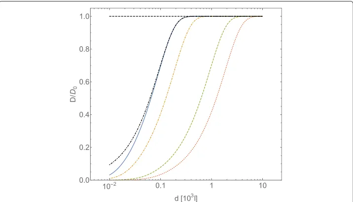
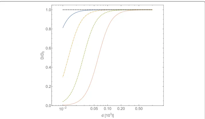
In Fig. 1 we plot the tracer self-diffusion coefficent behavior as a function of average distances among diffusing obstacles interacting through a Coulombic potential, following Eqs. (23) and (46); the intensity of Coulombic potential has been fixed toC¯Coul=0.7×102

while the value of the adimensionalized friction coefficienthas been changed. In this case it is necessary to choose 10−2in order to obtain sizeable effects on the value ofD/D0 at an average intermolecular distance of aboutl 103. Moreover, the value

of strongly affects the value of the intermolecular average distance among obstacles,

Fig. 1Normalized diffusion coefficientD/D0forA-type particles, computed with Eqs. (23) and (25), plotted vs. the intermolecular average distancedofB-type particles (expressed in adimensional unitsl). The

B-particles interact through a Coulombic potentialU_{= ¯}CCoull−1_{. TheA- andB-type particles are assumed} spherical, of equal radiusR, and equal massm. In adimensional units the interaction intensity is

¯

CCoul=UCoul(R)/(kBT), the friction coefficientγ=(kBTm)1/2R−1. The curves refer to a fixed value for the

which corresponds to a major deviation of the tracer self-diffusion coefficient from its Brownian value: the smaller the value ofis, the larger the distance among obstacles at which diffusion of tracers deviates from Brownian diffusion.

Assuming that the friction coefficient is given by Stokes’ law (15), the obtainedvalue corresponds toη1.5×10−4ηwater, whereηwateris the viscosity of water at temperature

T =300 K.

In Fig. 2 we plot the tracers self-diffusion coefficient behavior as a function of the aver-age distances among diffusing obstacles interacting through a Coulombic potential, for a fixed value of = 10−2and different values of the strength of Coulombic interaction among obstacles. In this case we observe that, as we increase the strength of Coulombic potential, the profile of tracers self-diffusion coefficient as a function of the average dis-tance among obstacles becomes sharper. Nevertheless, the intensity of the potential does not seem to affect the value of the average distance among obstacles at which the tracers self-diffusion coefficient deviates from its value in the absence of interactions.

We can conclude that the self-diffusion coefficient of tracers is mainly affected by the value of the friction coefficient. In the range of cases we have studied, the presence of interactions among obstacles affects only slightly the diffusion behavior of tracers, as it can be seen by comparing with the caseC¯Coul = 0. This effect can be interpreted as a

sort of “effective dynamical excluded volume” due to the presence of the obstacles; when the friction forces are weakened, the average speed both of the obstacles and the tracers increases and as a consequence the average free-flight time of tracers diminishes.

As mentioned above, the renormalized self-diffusion coefficient of tracers has been computed also in presence of obstacles interacting through a “dipole-dipole” potential

UDip(r)=CDipr−3 (49)

Fig. 2Normalized diffusion coefficientD_/D0, computed with Eqs. (23) and (25), forA-type particles vs. intermolecular average distancedofB-type particles (expressed in adimensional units). TheB-particles interact through a Coulombic potentialUCoul= ¯Cl−1. Conventions on units are the same of Fig. 1. The curves

refer to the fixed value₌0.01 of the friction coefficient, and to different values of the potential strength:

¯

CCoul=102_{(continuous line),CCoul}¯ ₌₁₀3_{(dot-dashed line),CCoul}¯ ₌₁₀4_{(dashed line), CCoul}¯ ₌₁₀5_(dotted

and a screened Coulombic potential, of a form close to the Debye-Hückel potential (which usually models electrostatic interactions in electrolytic solutions), that is

UCoulScr(r)= CCoulScr

exp [−r/λD]

r (50)

whereλDis the characteristic screening length scale, also called Debye length.

The potential in (50) can be rewritten in adimensional form:

UCoulScr(r=Rl)= ¯UCoulScr(l)=

UCoul(R)

kT

exp−l_λ−_¯1

D

l = ¯CCoulScr

exp−l_λ−_¯1

D

l (51)

where λ¯D = λD/Ris the adimensional screening length. As pointed out before, the

method proposed in the present paper is meaningful provided thatd R, therefore we take λ¯D ≥ 10, since for shorter screening length scales we don’t expect any effect of

the interactions among obstacles on the diffusion of tracers. For the screened Coulombic potential, Eq. (25) takes the form

x=x(d=Rl)= Td τA =

l2

2√3+ ¯CCoulScr

1

l2 +_lλ¯1

D

exp

−l−1

¯ λD

(52)

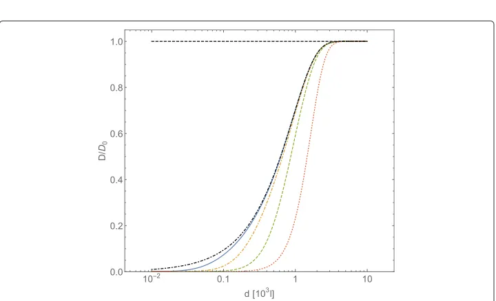
In Figs. 3 and 4 we show the behavior of tracers self-diffusion coefficient as a function of the concentration of interacting obstacles, in the case of “dipolar” and Coulomb screened interactions among obstacles, respectively. Different values for,C¯DipandC¯CoulScrhave

been chosen. In both cases we observe that the dependence of the tracers self-diffusion coefficient on the concentration of obstacles is much more affected by the value ofthan by the strength of the interaction potentials among obstaclesC¯Dip andC¯CoulScr, at least

in the explored range of parameters. This allows to conclude that also in this case the “effective dynamical excluded volume” mainly affects the tracers self-diffusion coefficient.

Fig. 3Normalized diffusion coefficientD/D0, computed with Eqs. (23) and (25), forA-type particles vs. intermolecular average distancedofB-type particles (expressed in adimensional units). TheB-type particles interact through a dipolar potentialU(r)=CDipr−3_{= ¯CDip(r/R)}−3_{. Conventions on adimensional units are} the same of Fig. 1. The curves refer to different choices of the friction coefficientand of the strengthCDip¯ of the potential energy:=0.05 andC¯=104_{(blue continuous line),=0.05 andC}¯₌₁₀6_(orange

Fig. 4Normalized diffusion coefficientD_/D0, computed with Eqs. (23) and (25), forA-type particles vs. intermolecular average distancedofB-type particles (expressed in adimensional units). TheB-type particles interact through the Coulombic screened potential given in (50). Conventions on adimensional units are the same of Fig. 1. The curves refer to different choices of the value of the friction coefficientand of the screening lengthλD=10 which set the strength of the potential energy:=0.05 andCCoulScr¯ =102(blue

continuous line),=0.05 andCCoulScr¯ =106_{(orange dot-dashed line),=0.01 andC}¯₌₁₀2_{(green dashed}

line),=0.01 andCCoulScr¯ =106_{(red dotted line). The case ofCCoulSCr}¯ _{=0 has been reported (black dot}

dashed line) for=0.05

Case of modification of the rescaled free-flight time distribution

As discussed in Section “Modification of the rescaled free-flight time distribution”, the proposed approach corresponds to the case where the characteristic timescale τ of Brownian collisions is much smaller than the transition time T_d. This corresponds to

intermolecular distancesdof the obstacles that are much larger than

mAkT

γ2

A

.

We remark that ifγ is given by the Stokes’ law (15) then the collision timeTddoes not

depend on the viscosity of the medium surrounding the particles but only on the ratio between the radii of theA- andB-type particles, on the functional form of the interaction potential between the obstacles, and on the strength of this potential. As in the previous section, we choose identicalA- andB-particles in order to introduce adimensional units. For a potential of the formU=Cr−n, Eq. (42) is rewritten as follows:

y(d=Rl)= 1

1+ 4d F(d)γA

3kTγB

1+ 1+8γA γB

2

= 1

1+₁₂1nC¯l−n (53)

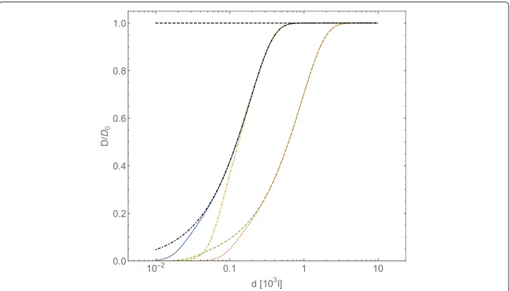
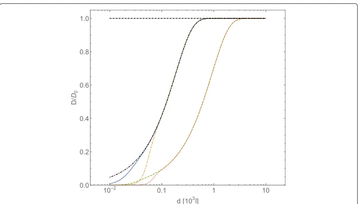
asγA = γB. In Figs. 5 and 6 we report the different patterns obtained forD/D0relative

to the tracers (A-particles) as a function of the average distancedbetween any pair of obstacles (B-particles) interacting through the Coulombic and dipolar potential.

Conclusions

Fig. 5Normalized diffusion coefficientD/D0, computed with Eqs. (41) and (42), forA-type particles vs. intermolecular average distancedofB-type particles (expressed in adimensional units). TheB-type particles interact through the Coulombic potentialU= ¯Cl−1. Conventions on adimentional units are the same of Fig. 1. The curves refer to different values of potential strength:CCoul¯ =102(continuous line),CCoul¯ =103 (dot-dashed line),CCoul¯ =104(dashed line),CCoul¯ =105(dotted line). The flat dashed line correspond to the caseCCoul¯ =0

be Brownian both for the tracers and the obstacles. Nevertheless, it would certainly be interesting in further studies to consider also other diffusive laws, in order to refine the model for crowded systems [20]. The CTRW framework is well suited for this, as it has been discussed in Section “Methods: continuous time random walk formalism”.

Fig. 6Normalized diffusion coefficientD/D0, computed with Eqs. (41) and (42), forA-type particles vs. intermolecular average distancedofB-type particles (expressed in adimensional units). TheB-type particles interact through a dipolar potentialU= ¯Cl−3_{. Conventions on adimensional units are the same of Fig. 1. The} curves refer to different values for potential strength:CDip¯ =102_{(continuous line), CDip}¯ ₌₁₀3_(dot-dashed

We found that the value of the Brownian self-diffusion coefficient of passive tracers is markedly affected by the randomly moving obstacles. The effects related to the presence and the strength of interactions among obstacles is in general less important than the “effective dynamical excluded volume” related to the friction constant. We stress that this result strongly depends on our estimation of the free-flight timeTd of passive tracers,

which is quite crude and seems to be the main aspect to be refined in our model in order to obtain more accurate results. An attempt to modify the estimation ofT_dis suggested in this article, resulting in the so called rescaled free-flight time distribution; in this case, the effect of friction is neglected and the slowing down of the passive tracers diffusion is due to only to the concentration of the obstacles and the strength of their mutual interactions. Nevertheless, this model has not yet a clear correspondence to real biological models.

Although we have adopted strong approximations and simplifications with respect to a realistic biological case of crowding, this work represents a first step in the analytic study of the value of the diffusion coefficient of passive tracers in the presence of interacting obstacles, and this fact can have relevant prospective consequences for applications to biology. For instance, the description of the complex network of biochemical reactions taking place in living cells could be markedly affected by the activation of long-range intermolecular interactions of the kind discussed in Ref. [15]. In particular, if we imagine a cytoplasm crowded by biomolecules interacting at a long distance, then molecules that would be driven to their targets only by diffusion could be considerably slowed down.

Appendix

In this section, we compute the probability distributionP(r,t) for the walker to be at locationr, at timet, following [17] and generalising the result to the three-dimensional case.

Letψ(r,t)be, as in Section “Methods: continuous time random walk formalism”, the probability density of making a displacementrin timetin a single motional event:

ψ(r,t)=(r) δ

t−|r| v0

The probability Q(r,t) of arriving at location r exactly at time t and to stop before randomly choosing a new direction satisfies the recursion relation:

Q(r,t)=

+∞

0 dt

d3r’Q(r−r’,t−t) ψ(r’,t)+δ(r)δ(t)

Jump model

In the Jump Model, particles wait at a particular location before moving instantaneously to the next one, the displacement being chosen according to the probability density(r), the waiting time before the jump being|r|/v0(because of theδ-function in the expression

ofψ(r,t)).

The three-dimensional formulation is straightforward in this case (and it appears for example in [18]). We have for the probability distributionP(r,t):

P(r,t)=

t

0

where(t)is the probability for not leaving a position up to timet:

(t)=

+∞

t

dt

d3rψ(r,t)

Passing to the Fourier-Laplace transform defined by:

f(k,s)=

+∞

0

dt e−st

d3reik·rf(r,t)

we get

Q(k,s)= 1 1−ψ(k,s) so that

P(k,s)= (s) 1−ψ(k,s)

The mean square displacementr2(t)is the inverse Laplace transform of the quantity

r2(s) = −kP(k,s)|k=0= −

(s) (1−ψ(k,s))2

kψ(k,s)+

2

1−ψ(k,s)(∇kψ(k,s)) 2

k=0

(54)

wherek is the Laplacian (k = ∂2/∂k2x +∂2/∂ky2+∂2/∂kz2) and∇k is the gradient

(∇k=(∂/∂kx,∂/∂ky,∂/∂kz)).

We now use the fact that in our case diffusion is isotropic. As discussed in Section “Methods: continuous time random walk formalism”, this allows to write

ψ(r,t)= φ(t) 4π (v0t)2δ(|

r| −v0t)

where we have introduced the waiting time distribution φ(t), which is the probabil-ity densprobabil-ity function that a single motional event has durationt, and is normalised by

_+∞

0 dtφ(t)=1. It is easy to show that

(s)= 1−φ(s)

s (55)

ψ(k=0,s)=φ(s) (56)

kψ(k,s)|k=0= −v20

d2

ds2φ(s) (57)

whereφ(s)is the Laplace transform ofφ(t).

Isotropy implies that∇kψ(k,s)|k=0=0, so that, replacing Eqs. (55), (56), (57) in Eq. (54)

we get

r2(s) = v 2 0

(1−φ(s))s· d2

ds2φ(s) (58)

Expanding expression (58) arounds0, we obtain

r2(s) v 2 0t2φ s2_tφ

Using Tauberian theorems [21], which relate the behavior of a functionf(t)at largetto that of its Laplace transform at smalls, we have at large times:

r2(t) v 2 0t2φ

which is the same as Eq. (10) of Section “Methods: continuous time random walk formalism”.

Velocity model

In the Velocity Model, each walker moves with constant velocity v0 between turning

points where a new direction and a new distance of flight are chosen according to the probability density(r). We have in this case:

P(r,t)=

t

0

dt

d3r’Q(r−r,t−t) (r,t)

where(r,t)represents the probability for a particle to make a displacementrin a time tin a single motional event and without stopping at timet. The explicit expression for (r,t)in three dimensions is given by:

(r,t)=pα,β(r|t)

d3r

_+∞

0

dtψ(r,t)θ(r− |r|)θ(t−t)δ(α−α)δ(β−β)

whereα,α,β,βare the angles which define the direction of vectorsrandrin a polar reference system andpα,β(r|t)is the conditional probability of making a displacement of

distancerin a time intervaltalong a vector whose orientation is specified by the anglesα andβ. Heaviside functionsθ(x)take into account time orderingt>tso that|r|−|r|>0, as the velocity is constant.

We again consider the Fourier-Laplace transform of the previous functions, obtaining:

Q(k,s)= 1 1−ψ(k,s) and

P(k,s)= (k,s) 1−ψ(k,s)

The mean square displacement r2(t) as a function of time is the inverse Laplace transform of the quantity:

r2(s) = −k=0P(k,s)|k=0= −

k(k,s)

(1−ψ(k,s))+

2∇kψ(k,s)· ∇k(k,s)

(1−ψ(k,s))2

+2(k,s)|∇kψ(k,s)|2

(1−ψ(k,s))3 +

(k,s)kψ(k,s)

(1−ψ(k,s))2

k=0

(59)

As we consider the isotropic case, we can rewriteψ(r,t)as

ψ(r,t)= φ(t) 4π (v0t)2δ(|

r| −v0t)

Under this hypothesis(r,t)has the form:

(r,t)=δ(|r| −v0t) v2₀t2

d3r

_+∞

0

dt φ(t ₎ 4πv2₀t2δ(|r

_{| −v} 0t)

×θ(r− |r|)θ(t−t)δ(α−α)δ(β−β)

The isotropy hypothesis implies ∇kψ(k,s)|k=0=0. Equation (59) then reduces to:

r2(s) = − 1 (1−ψ(k,s))

k(k,s)+(

k,s)kψ(k,s)

(1−ψ(k,s))

k=0

It is easy to show that:

(k=0,s)= 1−φ(s)

s (61)

and

k(k,s)|k=0= −v20

d2 ds2

1−φ(s) s

(62)

whereφ(s)is the Laplace transform ofφ(t).

Replacing the Fourier-Laplace transforms (56), (57), (61), (62) in Eq. (60) we obtain:

r2(s) = v 2 0

(1−φ(s))

d2 ds2

1−φ(s) s

+ 1

s d2 ds2φ(s)

(63)

Expanding expression (63) around zero, we obtain:

r2(s) v 2 0t2φ s2_tφ

and using Tauberian theorems [21], we have at large times:

r2(t) v 2 0t2φ

tφ t as in the Jump Model.

Competing interests

The authors declare that they have no competing interests.

Authors’ contributions

MG and EF developed the application of the Continuous Time Time Random Walk formalism to the special problem considered. IN and ID contributed to the numerical analysis and to the discussions defining the model. MP proposed the problem and supervised the overall development of the work. All authors participated in the scientific discussions and to the writing and editing of the manuscript. All authors read and approved the final manuscript.

Acknowledgments

The authors wish to thank F. Piazza and R. Lima for useful comments and suggestions. This work was supported by the Seventh Framework Programme for Research of the European Commission under FET-Open grant TOPDRIM (Grant No. FP7-ICT-318121).

Author details

1_{Aix-Marseille Université, Marseille, France.}2_{CNRS Centre de Physique Théorique UMR7332, 13288 Marseille, France.} 3_{Centre d’Immunologie de Marseille-Luminy, Aix Marseille Université UM2, Inserm, U1104, CNRS UMR7280, 13288}

Marseille, France.

Received: 10 December 2015 Accepted: 19 March 2016

References

1. Chernov AA. Replication of multicomponent chain by the lighting mechanism. Biophysics. 1967;12:336. 2. Harris T. Diffusion with collision between particles. J Appl Prob. 1965;2:323.

3. Solomon F. Random walks in a random environment. Ann Prob. 1975;3:31.

4. Boldrighini C, Cosimi G, Frigio S, Pellegrinotti A. Computer simulations for some one-dimensional models of random walks in fluctuating random environment. J Stat Phys. 2005;121:361.

5. Boldrighini C, Minlos RA, Pellegrinotti A. Random walks in quenched i.i.d. space-time random environment are always a.s. diffusive. Prob Theor Related Fields. 2004;129:133.

6. Dolgopyat D, Keller G, Liverani C. Random walk in markovian environment. Ann Prob. 2008;36:1676.

7. Dolgopyat D, Liverani C. Non-perturbative approach to random walk in markovian environment. Electron Comm Probab. 2009;14:245.

8. Saxton MJ. Single-particle tracking: the distribution of diffusion coefficient. Biophys J. 1996;70:1250. 9. Lucas JS, Zhang Y, Dudko OK, Murre C. 3d trajectories adopted by coding and regulatory dna elements:

first-passage times for genomic interactions. Cell. 2014;158:339.

10. Montroll EW, Weiss GH. Random walks on lattices, ii. J Math Phys. 1965;6:167.

11. Tabaka M, Kalwarczyk T, Szymanski J, Hou S, Holyst R. The effect of macromolecular crowding on mobility of biomolecules, association kinetics and gene expression in living cells. Front Phys. 2014;2(54).

doi:10.3389/fphy.2014.00054.

13. Preto J, Floriani E, Nardecchia I, Ferrier P, Pettini M. Experimental assessment of the contribution of electrodynamic interactions to long-distance recruitment of biomolecular partners: Theoretical basis. Phys Rev E. 2012;85:041904. 14. Nardecchia I, Spinelli L, Preto J, Gori M, Floriani E, Jaeger S, Ferrier P, Pettini M. Experimental detection of

long-distance interactions between biomolecules through their diffusion behavior: Numerical study. Phys Rev E. 2014;90:022703.

15. Preto J, Pettini M, Tuszynski J. Possible role of electrodynamic interactions in long-distance biomolecular recognition. Phys Rev E. 2015;91:052710.

16. Preto J, Nardecchia I, Jaeger S, Ferrier P, Pettini M. In: Cifra M, Fels D, editors. Long-range resonant interactions in biological systems: theory and experiment. Chapter 11 of the e-book “Fields of the Cell”. Kerala India: Publishing House Research Signpost; 2015.

17. Zumofen G, Klafter J. Scale-invariant motion in intermittent chaotic systems. Phys Rev E. 1993;47:851. 18. Klafter J, Blumen A, Schlesinger MF. Stochastic pathway to anomalous diffusion. Phys Rev A. 1987;35:3081. 19. Stroppolo ME, Falconi M, Caccuri AM, Desideri A. Superefficient enzymes. Cell Mol Life Sci. 2001;58:1451. 20. Banks DS, Fradin C. Anomalous diffusion of proteins due to molecular crowding. Biophysical journal. 2005;89(5):

2960–2971.

21. Feller W. An Introduction to Probability Theory and Its Applications, vol II, chap XVIII. New York: Wiley; 1971.

• We accept pre-submission inquiries

• Our selector tool helps you to find the most relevant journal • We provide round the clock customer support

• Convenient online submission • Thorough peer review

• Inclusion in PubMed and all major indexing services • Maximum visibility for your research

Submit your manuscript at www.biomedcentral.com/submit